Lat. Am. j. solids struct. vol.12 número3

(1)

Abstract

Despite the availability of large number of empirical and semi-empirical models, the problem of penetration depth prediction for concrete targets has remained inconclusive partly due to the complexity of the phenomenon involved and partly because of the limitations of the statistical regression employed. Conventio-nal statistical aConventio-nalysis is now being replaced in many fields by the alternative approach of neural networks. Neural networks have advantages over statistical models like their data-driven nature, model-free form of predictions, and tolerance to data errors. The objective of this study is to reanalyze the data for the prediction of penetration depth by employing the technique of neural networks with a view towards seeing if better predic-tions are possible. The data used in the analysis pertains to the ogive-nose steel projectiles on concrete targets and the neural network models result in very low errors and high correlation coefficients as compared to the regression based models.

Keywords

Neural Networks; penetration depth; concrete targets; projectile.

Neural Network Approach for Estimation of Penetration

Depth in Concrete Targets by Ogive-nose Steel Projectiles

1 INTRODUCTION

Concrete has been widely used over many years by military and civil engineers in the design and construction of protective structures to resist impact and explosive loads. Potential missiles in-clude kinetic munitions, vehicle and aircraft crashes, fragments generated by military and terror-ist bombing, fragments generated by accidental explosions and other events (e.g. failure of a pres-surized vessel, failure of a turbine blade or other high-speed rotating machines), flying objects due to natural forces (tornados, volcanos, meteoroids), etc. These missiles vary broadly in their sizes and shapes, impact velocities, hardness, rigidities, impact attitude (i.e. obliquity, yaw, tumbling, etc.) and produce a wide spectrum of damage in the target (Li et al., 2005).

In the past 60 years, a large amount of laboratory tests had been conducted in various coun-tries (Kennedy, 1976; Sliter 1980; Williams, 1994; Corbett et al., 1996). Based on these available

M. Hosseinia A. Dalvandb

a_{Dept. of Civil Engineering, Lorestan}

University, Khoramabad, P.O. Box 465, Iran.

b_{Dept. of Civil Engineering, Lorestan}

University, Khoramabad, Iran.

Corresponding autor:

a_{mo_hosseini78@yahoo.com} b_{alidalvand85@yahoo.com}

http://dx.doi.org/10.1590/1679-78251200

(2)

Latin A m erican Journal of Solids and Structures 12 (2015) 492-506

test data, empirical formulae have been proposed to predict the penetration depth on concrete target. Empirical formulae on penetration depth, perforation limit and scabbing limit in a thick concrete target had been reviewed by Kennedy (1976), which covered most of the test data in the US and European till 1970s. Comparison between various empirical formulae and published test data was conducted by Williams (1994). Among the most commonly used formulae are the Pettry formula, the Army Corps of Engineers formula (ACE), Ballistic Research Laboratory formula (BRL) and the National Defence Research Committee (NDRC) formula.

In this study, by using the projectile and target parameters, proposed a dimensionless empiri-cal formula to predict the rigid projectile penetration depth of concrete target. It is shown that these dimensionless formula is capable of representing test data on penetration depth in a broad range of impact velocity as long as the projectile deformation is negligible, which covers the ap-plicable range of empirical formulae.

2 AVAILABLE FORM ULA FOR LOCAL CONCRETE DAM AGE PREDICTION

The most commonly formula used to predict various components of local impact effects of hard missile on concrete structure in USA was modified Petry formula. It is the oldest of available empirical formulae, and developed originally in 1910. According to Petry the penetration depth x (inches) can be predicted as (Kennedy, 1976):

2

10

12 log 1

215000

p p

V

x K A (1)

This equation was derived from the equation of motion which states that the component of drag-resisting force depends upon square of the impacted velocity, and the instantaneous resisting force is constant. In above equation, A_p represents the missile section pressure (psi).K_p is

concre-te penetrability coefficient, it depends upon the strength of concreconcre-te and on the degree of reinfor-cement. It equals to 0.00426 for normal reinforced cement concrete, 0.00284 for special reinforced cement concrete (front and rear face reinforcement are laced together with special ties), and 0.00799 for massive plain cement concrete.

Before 1943, The Ordnance Department of the US Army and Ballistic Research Laboratory (BRL) done many experimental works on local impact effects of hard missile on concrete structu-re, based on those results Army Corp of Engineers developed the ACE formula (Kennedy, 1976; Chelapati et al., 1972; ACE 1946):

1.5 0.215

3 282.6

0.5 1000

c

x W V

d

d f d

(2)

For the calculation of penetration depth (x) of concrete impacted by hard missile, Ballistic

(3)

1.33 0.2

3 427

1000

c

x W V

d

d f d (3)

Modified National Defense Research Committee (NDRC) Formula: In 1946, the National De-fense Research Committee (NDRC) proposed the following formula for predicting the penetration depth (Kennedy, 1976; NDRC 1946; Kennedy, 1966):

0.5 1.8 4

1000

x NKW V

d d d for 2

x

d (4)

1.8 1

1000

x NKW V

d d d for 2

x

d (5)

K is the concrete penetration factor and is given as a function of concrete strength f_c as follows:

180

c K

f (6)

N is the missile nose shape factor. 1.0 For average bullet nose (spherical end), 0.84 for blunt

nosed bodies and 1.14 for very sharp nose. All the above empirical formula applied only for non-reinforced structures impacted by solid missile.

Ammann and Whitney (A&W) formula was proposed to predict penetration of concrete target against the impact of explosively generated small fragments at relatively higher velocities. Accor-ding to Kennedy (Kennedy, 1976) this formula can predict penetration of explosively generated small fragments traveling at over 1000 ft/sec.

1.8 0.2

3 282

1000

c

x M V

N d

d f d (7)

In this formula _N*_{is the nose shape function same as defined in NDRC formula.}

Where in the above equations:

d is the diameter of the missile in inches W is the weight of the missile in pounds

c

f is the compressive strength of concrete in Psi

And V missile velocity in _ft/sec2

Haldar Hamieh (Halder and Hamieh, 1984) suggested the use of an impact factor I_a, defined

by:

2

3

a c MN V I

(4)

where I_a is impact factor and it is a dimensionless term, N* is the nose shape factor defined in

the modified NDRC formula. For penetration depth (x):

0.2251_a 0.0308

x

I

d for 0.3 Ia 4.0 (9)

0.0567 _a 0.674

x

I

d for 4.0 Ia 21 (10)

0.0299 _a 1.1875

x

I

d for 21 Ia 455 (11)

Li and Chen (Li and Chen, 2003) further develop Forrestal et al. (1994) model and proposed semi empirical or semi analytical formulae for the penetration depth (x). The formulae are in dimensional homogenous form, and defines nose shape factor analytically.

(1 ( _{)) 4}

4 1

k

x _N kI

d I

N

for x 5

d (12)

1 ( )

2 ln

1 ( )

4

I

x _N

N k

d k

N

for x 5

d (13)

Where

2

3 1

c MV I

S f d (14)

3 1

C M N

N d (15)

where N, I , and N* are the impact function and the geometry function and nose shape factor

respectively. S is an empirical function of fc (MPa) and is given by:

0.5 72_c

S f (16)

The above equations are applicable for x d ≥ 0.5, and reduced the results obtained by

Forres-tal et al. (1996) for an ogive nose projectile. ForresForres-tal et al. (1994, 1996) and Frew et al. (1998) suggested that if x d ≥ 5.0 than k = 2.0, this statement is strengthened by the instrumented

experiments in (Forrestal et al. 2003), and with penetration experiments with wide range of pro-jectile diameter (Frew et al. 2000) And Li and Chen (2003) recommended x d < 5.0, for small

to medium penetration depths:

0.707 h

k

d (17)

(5)

Latin A m erican Journal of Solids and Structures 12 (2015) 492-506 3 EXPERIM ENTAL DATA

The data used in the analysis is taken from Frew et al. (1998); Forrestal et al. (1994); Forrestal et al. (1996); Forrestal et al. (2003) which makes a total of 70 data points. The data consists of four parameters viz. projectile diameter (d), projectile velocity (V ), compressive strength of

con-crete (f_c), projectiles weight (W). The range of these parameters for the data is given in Table 1.

S. NO. Parameter Range

Basic Parameters

1 Projectile diameter,d (mm) 12.9 - 76.2

2 Projectile velocity, V (m/s) 139.3 - 1225

3 Projectile weight (N) 0.63 - 129

4 compressive strength of concrete f_c (MPa) 13.5 - 62.8 Non-Dimensional Parameters

1 2 3

c

MV Sf d 1.66 164.06

Table 1: Range of parameters for the data of experimental details of projectiles and concrete targets (70 data points).

4 PROPOSED M ODEL

The empirical model used for the prediction of penetration depth in concrete target is:

2 2

1 ₃ 3

C

c

x MV

C C

d Sf d (18)

Where, C₁, C₂, C₃ are the model parameters, M is projectiles mass and S is an empirical

fun-ction of fc (MPa) and is given by (Forrestal et al., 1996):

0.544 82.6_c

S f (19)

Parameters C₁ to C₃, have been determined by regression analysis for data involving (a)

projec-tiles with CRH=3 to 4.25 and (b) projecprojec-tiles with CRH= 6. Thus giving tow regression models:

0.85 2

3 1

c

x MV

d Sf d for projectiles with CRH=3 to 4.25 (20)

0.85 2

3

1.6 1

c

x MV

d Sf d for projectiles with CRH= 6 (21)

(6)

Where (CRH) is caliber-radius-head of the projectiles.

The performance of various regression models presented above has been compared in Table 2 with the help of mean percentage error. It is observed from this table that the mean error of Pro-posed model is lower than other models.

Number of data

Mean Percentage Error %

BRL ACE NDRC Li&Chen A&W Pettry Halder Eqs. (20)-(21)

70 16.3 28.2 31.7 12.6 12 99.2 56 10.3

Table 2: Mean percentage error for different models.

5 NEURAL NETWORK M ODEL

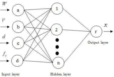
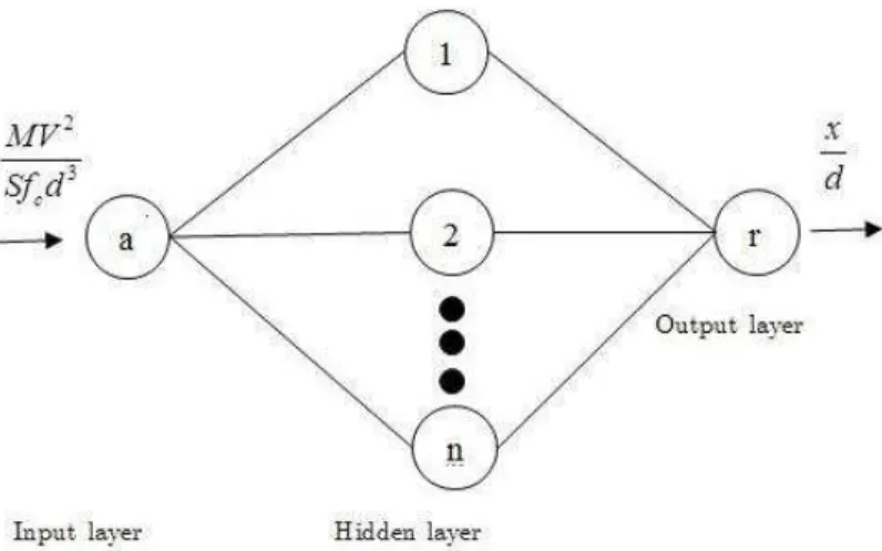
The manner in which the data are presented for training is the most important aspect of the neu-ral network method. Often this can be done in more than one way, the best configuration being determined by trial-and-error. It can also be beneficial to examine the input/output patterns or data sets that the network finds difficult to learn. This enables a comparison of the performance of the neural network model for these different combinations of data. In order to map the causal relationship related to the penetration depth, two separate input-output schemes (called Model A1 and Model A2) were employed, where the first took the input of raw causal parameters whi-le the second utilized their non-dimensional groupings. This was done in order to see if the use of the grouped variables produced better results? The Model A1 thus takes the input in the form of causative factors namely,W,V , d, and f_c yields the output, the penetration depth, x, while Model A2 employs the input of grouped dimensionless variables namely, 2 3

c

MV Sf d , and

yields the corresponding dimensionless output x d. Thus, the two models are:

Model A1: x f W V d f, , , _c (22)

Model A2: 2

3

c

x MV

f

d Sf d (23)

The input and output variables involved in the above two models were first normalized within the range 0 to 1 as follows:

min

max min

N

x x x

x x (24)

Where x_N is the normalized value of x; x_max and x_min are the maximum and minimum values of

variable, x. This normalization allowed the network to be trained better.

The current study used the data considered above (70 data points) for the prediction of pene-tration depth. The training of the above two models was done using 67% of the data (46 data points) selected randomly. Validation and testing of the proposed models was made with the help

)

(

(7)

of the remaining 33% of observations (24 data points), which were not involved in the derivation of the model.

Three neuron models namely, tansig, logsig and purelin, have been used in the architecture of the network with the back-propagation algorithm. In the back-propagation algorithm, the feed-forward (FFBP) and cascade-feed-forward (CFBP) type network was considered. Each input is weigh-ted with an appropriate weight and the sum of the weighweigh-ted inputs and the bias forms the input to the transfer function. The neurons employed use the following differentiable transfer function to generate their output:

Log-Sigmoid Transfer Function: 1

1 ij i j

j ij i j _{w x}

i

y f w x

e

(25)

Linear Transfer Function: _j _{ij i} _j _{ij i} _j

i i

y f w x w x (26)

Tan-Sigmoid Transfer Function:

2 2

1

1 ij i j

j ij i j _{w x}

i

y f w x

e

(27)

The weight, w, and biases, , of these equations are determined in such a way as to minimize the energy function. The Sigmoid transfer functions generate outputs between 0 and 1 or -1 and +1 as the neuron's net input goes from negative to positive infinity depending upon the use of log or tan sigmoid. When the last layer of a multilayer network has sigmoid neurons (log or tan), then the outputs of the network are limited to a small range, whereas, the output of linear output neu-rons can take on any value.

Further, in order to see if advanced training schemes provide better learning than the basic back propagation, a radial basis function (RBF) network was also used which though requires more neurons but it is sometimes more efficient. The Radial basis transfer function is given by:

2

ij i j

w x

j ij i j

i

y f w x e 28)

The optimal architecture was determined by varying the number of hidden neurons. The op-timal configuration was based upon minimizing the difference between the neural network predic-ted value and the desired output. In general, as the number of neurons in the layer is increased, the prediction capability of the network increases in beginning and then becomes stationary.

The performance of all neural network model configurations was based on the Mean Percent Error (MPE), Mean Absolute Deviation (MAD), Root Mean Square Error (RMSE), Correlation Coefficient (CC), and Coefficient of Determination, _R2_{, of the linear regression line between the} predicted values from the neural network model and the desired outputs.

The training of the neural network models was stopped when either the acceptable level of error was achieved or when the number of iterations exceeded a prescribed maximum. The neural network model configuration that minimized the MAE and RMSE and optimized the _R2_was selected as the optimum and the whole analysis was repeated several times.

(

( )

)

(8)

Latin A m erican Journal of Solids and Structures 12 (2015) 492-506 6 SENSITIVITY ANALYSIS

Sensitivity tests were conducted to determine the relative significance of each of the independent parameters (input neurons) on the penetration depth (output) in both of the models given by Eqs. (22) and (23). In the sensitivity analysis, each input neuron was in turn eliminated from the model and its influence on prediction of penetration depth was evaluated in terms of the MPE, MAD, RMSE, CC and _R2_{criteria. The network architecture of the problem considered in the} present sensitivity analysis consists of one hidden layer with thirteen neurons for model-A1and fourteen neurons for model-A2 and the value of epochs has been taken as 100.

The comparison of different neural network models, with one of the independent parameters removed in each case is presented in Table 3. The influence of the removal of one independent parameter at a time has been studied for all four parameters. The results in Table 3 show that for Model A1, the velocity of projectile, V, and compressive strength of concrete,f_c , are the two

most significant parameters for the prediction of penetration depth. The variables in the order of decreasing level of sensitivity for Model A1 are: V, f_c, d and W.

2

R

CC RMSE

MAD MPE

Input variables

0.992 0.996

5.01 5.1

-0.34 All Eq.(22)

0.2 0.610

52.4 55.5

-11.7

V

No

0.97 0.980

8.3 5.0

-0.26 No W

0.98 0.988

5.4 5.1

0.51

d

No

0.95 0.970

12.4 8.7

2.4 c

f

No

Table 3: Sensitivity analysis for Model A1 with Feed Forward Back Propagation.

Note: MPE = Mean Percent Error; MAD = Mean Absolute Deviation; RMSE = Root Mean Square Error; CC = Correlation Coefficient; _R2_{= Coefficient of Determination.}

Input MPE MAD RMSE CC _R2

Eq.(23) 3.25 9.6 3.5 0.988 0.978

Table 4: analysis results for Model A2 with ANN.

7 NUM ERICAL RESULTS

(9)

The information on number of nodes required to achieve minimum error taken in the case of each training scheme used (i.e. FFBP, CFBP, and RBF) is shown in Table 5 for Model A1 and A2. As a matter of general information, which is not of real significance in this study, it can be seen that the cascade correlation algorithm, designed for efficient training, trained the network with fewer epochs than the FFBP network, but the RBF network was trained in a significantly less number of epochs, indicating its training efficiency.

Model Algorithm Network Configuration Learning Rate Momentum Function

I H O 0.5 0.7

Model A1

FFBP 4 13 1 0.5 0.7

CFBP 4 15 1 0.5 0.7

RBF 4 60 1 0.5 0.7

Model - A2

FFBP 1 14 1 0.5 0.7

CFBP 1 17 1 0.5 0.7

RBF 1 55 1 0.5 0.7

Table 5: Network Architecture.

Note: I, H, O indicate number of input, hidden, and output nodes, respectively; FFBP = Feed-Forward Back Propagation; CFBP = Cascade-Forward Back Propagation; and RBF = Radial Basis Function.

The network architecture of the two models, given by Eqs. (22)-(23), is given in Figs. 1-2 res-pectively for BP/RBF training scheme. The error estimation parameters (MPE, MAD, RMSE, CC and _R2_{), on the basis of which the performance of a model is assessed, are already given in} Tables 3-4.

Figure 1: Model A1: use of raw variables.

(10)

Latin A m erican Journal of Solids and Structures 12 (2015) 492-506 Figure 2: Model A2: use of grouped variables

Figure 3: Epochs versus squared error of raw variables by back propagation.

Figure 4: Epochs versus squared error of grouped variables by back propagation.

0 5 10 15 20 25 30 35 40 45

0 5 10 15 20 25

epoch

S

qu

ar

ed

E

rr

or

Training validation test

0 5 10 15 20 25 30 35 40

0 1 2 3 4 5 6 7 8 9 10

epoch

S

qu

ar

ed

E

rr

or

(11)

Latin A m erican Journal of Solids and Structures 12 (2015) 492-506 No. of neuron Input weights

Output

weights _{Input biases}

a b c d r

1 -1.83 -2.107 -0.41 1.1 1.6991 2.4981

2 1.83 1.17 0.83 0.9 -1.9403 -0.7743

3 -0.34 1.78 2.17 -0.3 0.0503 1.6994

4 -1.73 0.49 -1.39 -1.6 -0.71 0.3887

5 1.18 2.26 -0.66 -0.04 -0.852 -0.9643

6 -0.69 -0.97 -2.45 0.66 -0.438 0.3199

7 0.56 -1.06 -1.81 1.05 -0.3551 0.3068

8 2.48 1.61 0.89 1.52 1.6615 0.1549

9 -0.89 -1.48 -1.395 1.084 0.4994 -1.0383

10 1.25 -1.39 0.9 -1.09 0.4744 0.5866

11 -4 -1.41 0.084 -0.888 -1.0161 -0.168

12 1.859 0.2271 -2.37 4.16 0.4721 1.5101 13 0.298 0.968 0.073 1.92 0.0715 -3.0808

Table 6: Connection weights and biases (Refer to Figure 1). (Output bias= -1.6).

No. of neuron

Input weights Output weights _Input biases

a r

1 20.015 -1.444 -19.197

2 -19.5954 -1.2504 16.8313

3 -19.1899 0.0419 14.1144

4 -20.1306 -0.0974 9.3933

5 19.4844 -0.0327 -7.9381

6 -20.0332 -0.0863 4.517

7 -19.7706 -0.1156 2.1064

8 -19.4814 -0.1696 -2.9871

9 19.8566 -0.0404 3.2438

10 -19.6182 -0.12 -7.6026

11 18.8785 0.255 12.0185

12 -19.8142 0.137 -13.210

13 -19.6967 -0.0704 -16.386

14 -19.5918 -0.0855 -19.587

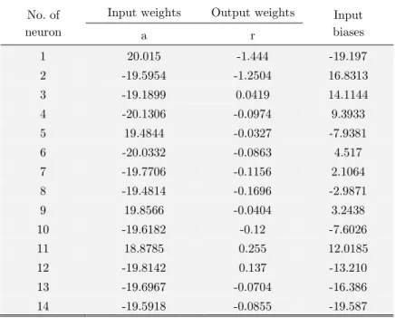
Table 7: Connection weights and biases (Refer to Figure 2). (Output bias= -0.52).

(12)

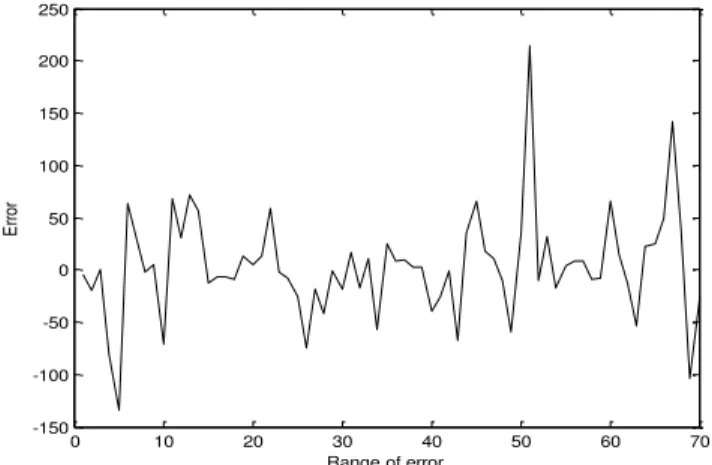
Latin A m erican Journal of Solids and Structures 12 (2015) 492-506 Figure 5: Percentage error for Model-A1.

Figure 6: Percentage error for Model A2.

The examination of Tables 3-4 and Figs. 7-8 show that when it comes to overall accuracy of predicting penetration depth, all error criteria viewed together point out that the simple feed forward network trained using the common BP algorithm is either as good as or even slightly better than more sophisticated networks.

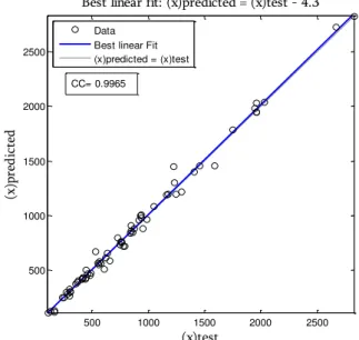
It also shows that the use of grouped variables as input (Model A2) may be less beneficial than that of the raw variables (Model A1), provided an appropriate training scheme is chosen, where perhaps grouping of variables had resulted in evening out their scale effects. The most sui-table network, FFBP Model A1, has the highest CC = 0.996 and _R2_{= 0.992; and lowest MPE} = 0.34, MAD = 5.1, and RMSE = 5.01. All the ANN models featured small RMSE during trai-ning; however, the value was slightly higher during validation. The models showed consistently good correlation throughout the training and testing.

In the end therefore the network configuration (FFBP Model A1) along with corresponding weight and bias matrix given in Table 6 is recommended for general use in order to predict the penetration depth.

The value of MAD in the prediction of penetration depth by regression model given in Table 2 (10.3% for all data) may be compared with the performance of neural network model A1 whe-rein the MAD value is only 5.1%. The histogram of percentage error in the prediction of

penetra-0 10 20 30 40 50 60 70

-150 -100 -50 0 50 100 150 200 250

Range of error

E

rr

or

0 10 20 30 40 50 60 70

-20 -15 -10 -5 0 5 10 15 20

Range of error

E

rr

(13)

tion depth by regression and the two neural network models is shown in Fig. 9. This clearly indi-cates the supremacy of the neural network model over the regression model and the one available in literature. Further, the neural networks have advantages over statistical models like their data-driven nature, model-free form of predictions, ability to implicitly detect complex nonlinear rela-tionships between dependent and independent variables, ability to detect all possible interactions between predictor variables and tolerance to data errors.

The predictions should be preferably used within the range of the experimental data because of the possibility of intervention of new phenomena when used beyond the range.

Figure 7: Observed versus predicted x (mm) for Model A1.

Figure 8: Observed versus predicted x d for Model A2.

500 1000 1500 2000 2500

(x)test

(x

)p

re

d

icte

d

Best linear fit: (x)predicted = (x)test - 4.3

Data Best linear Fit (x)predicted = (x)test

CC= 0.9965

10 20 30 40 50 60 70 80 90 10

20 30 40 50 60 70 80 90

(x/d)test

(x

/d

)p

rd

icte

d

Best linear fit: (x/d)predicted=0.97(x/d)test+0.92

(14)

Figure 9: Histogram of percentage error in different models.

8 CONCLUSIONS

A regression based empirical model has been developed based upon the data available in literatu-re for the pliteratu-rediction of penetration depth in concliteratu-rete target by ogive-nose steel projectiles. The proposed regression model is more accurate predictor of penetration depth than the other availa-ble in literature.

Predictions based on the use of raw dimensioned data (V ,W,f_c and d) in the development of

neural networks were better than those based on the grouped dimensionless forms of the data,

2 3

c

MV Sf d . The neural network with one hidden layer was selected as the optimum network to

predict penetration depth. The network configuration of Model A1 with FFBP is recommended for general use in order to predict the of penetration depth in concrete target by ogive-nose steel projectiles.

The neural network model is far better than the regression based models proposed as well as the other available in literature for the prediction of the penetration depth in concrete target by ogive-nose steel projectiles.

References

ACE, (1946). Fundamentals of protective structures. Report AT120 AT1207821, Army Corps of Engineers, Office of the Chief of Engineers.

Adeli, H., Amin, A.M., (1985). Local effects of impactors on concrete structures. Nucl. Eng. Des. 88: 301-317. Beth, R.A., (1941). Penetration of projectiles in concrete. PPAB Interim Report No. 3, November 1941.

Chelapati, C.V., Kennedy, R.P., Wall, I.B., (1972). Probabilistic assessment of hazard for nuclear structures. Nucl. Eng. Des. 19: 333-334.

Corbett, G.G, Reid, S.R, Johnson, W., (1996). Impact loading of plates and shells by free-flying projectiles, a review. Int. J. Impact Eng. 18: 141-230.

Forrestal, M.J., Altman, B.S., Cargile, J.D., Hanchak, S.J., (1994). An empirical equation for penetration depth of ogive-nose projectiles into concrete targets. Int. J. Impact Eng. 15(4): 395-405.

0 20 40 60 80 100

0_10% 10_20% 20_30% 30_40%

Per

ce

nt

ag

e

of

dat

a

Range of error

Proposed model ANN model A1 ANN model A2

(15)

Latin A m erican Journal of Solids and Structures 12 (2015) 492-506 Forrestal, M.J., Frew, D.J., Hanchak, S.J., Brar, N.S., (1996). Penetration of grout and concrete targets with ogive-nose steel projectiles. Int. J. Impact Eng. 18(5): 465-476.

Forrestal, M.J., Frew, D.J., Hickerson, J.P., Rohwer, T.A., (2003). Penetration of concrete targets with decelera-tion-time measurements. Int. J. Impact Eng. 18: 479-497.

Frew, D.J., Forrestal, M.J., Hanchak, S.J., (2000). Penetration experiments with limestone targets and ogive-nose steel projectiles. ASME J Appl Mech. 67: 841-845.

Frew, D.J., Hanchak, S.J., Green, M.L., Forrestal, M.J., (1998). Penetration of concrete targets with ogive-nose steel rods. Int. J. Impact Eng. 21: 489-497.

Haldar, A., Hamieh, H., (1984). Local effect of solid missiles on concrete structures. ASCE J Struct Div. 110(5): 948-960.

Kennedy, R.P., (1976). A review of procedures for the analysis and design of concrete structures to resist missile impact effects. Nucl. Eng Des. 37: 183-203.

Kennedy, R.P., (1966). Effects of an aircraft crash into a concrete reactor containment building. Anaheim, CA: Holmes & Narver Inc.

Li, Q.M., Chen, X.W., (2003). Dimensionless formulae for penetration depth of concrete target impacted by a non-deformable projectile. Int. J Impact Eng. 28(1): 93-116.

Li, Q.M., Reid, S.R., Wen, H.M., Telford, A.R., (2005). Local impact effects of hard missiles on concrete targets. International Journal of Impact Engineering. 32: 224-284.

NDRC., (1946). Effects of impact and explosión. Summary Technical Report of Division 2, vol. 1, National Defen-ce Research Committee, Washington, DC.