Are price limits on futures markets that cool? evidence from the brazilian merchantile & futures exchange

Rio de Janeiro

Escola

de

Pós-Graduação

em

Economia

Fundação

Getulio

Vargas

Are

price

limits

on

futures

markets

that

cool?

Evidence

from

the

Brazilian

Merchantile

&

Futures

Exchange

Dissertação submetida à Escola de Pós-Graduação em Economia da

Fundação Getulio Vargas como requisito para obtenção do Título de

Mestre em Economia

Aluno Marco Aurélio dos Santos Rocha

Rio de Janeiro

Fundação

Getulio

Vargas

Are

price

limits

on

futures

markets

that

cool?

Evidence

from

the

Brazilian

Merchantile

&

Futures

Exchange

Dissertação submetida à Escola de Pós-Graduação em Economia da

Fundação Getulio Vargas como requisito para obtenção do Título de

Mestre em Economia

Aluno Marco Aurélio dos Santos Rocha

Banca Examinadora

Marcelo Fernandes (Orientador, EPGE/FGV)

Marco Antonio Bonomo (EPGE/FGV) Walter

Are

price

limits

on

futures

markets

that

cool?

Evidence

from

the

Brazilian

Merchantile

&

Futures

iv

Agradecimentos

A Deus, sempre.

A minha esposa, pelo seu amor, alegria e dedicação

incondi-cionais.

AsdemaismulheresdaminhavidaJoana,Lina,Flávia,e,agora,

Amandapelocarinhoeamor.

A minha famíla pelos exemplos de vida e,em especial, aomeu

sogro Nelson Moreira de Carvalho, que também contribuiu para

tornarmenossofrívelomeuinglês.

Ao parceiro eorientador Marcelo Fernandes pela porta sempre

abertaepelaamizade.

Aos camaradas Julio Cesar and Margareth pela companhia e

pelosmomentosdivididos.

Aos amigos de sempre e aos que aqui fiz pelo apoio,

principal-mentenosdiasdifíceis.

Ao BancoCentral doBrasil pelo patrocínio epelo apoio

materi-alizadopormeiodoDeban (DepartamentodeOperações Bancáriase

Sistema de Pagamentos), particularmente com a ajuda de Luiz

FernandoCardosoMacieleSérgioJosé Ceia.

Ao meuorientadornoBancoCentralMarcosJoséRodrigues

Tor-respordespertaromeuinteressepeloassunto.

À BolsadeMercadoriaeFuturos,representada porVerdiRosae

Cicero Vieira,peloacessoaosdadoseinformaçõesvitais àconclusão

destetrabalho.

Aos funcionáriosda EPGE, queorgulhosamentefiguramna lista

dosamigosquefizaqui,emespecialao NúcleodeComputação,que,

representado por Alexandre Rademaker, foi fundamental ao bom

termodapesquisa.

Especialmente, agradeço aos professores Fritz José Barbosa e

JandirMoraesFeitosaJr., que sãoosresponsáveispeloiníciodessa

v Abstract

This paper investigatesthe impact of price limitson the

Brazil-ianfuturemarketsusinghighfrequencydata. Theaimistoidentify

whether there is a cool-off or amagnet effect. For that purpose,

weexamine atick-by-tickdata setthatincludesallcontractsonthe

SãoPaulo stock index futures traded on the Brazilian Mercantile

andFutures Exchange from January 1997to December 1999. Our

main finding isthat price limits drivebackprices astheyapproach

thelowerlimit. Thereisastrongcool-offeffectofthelowerlimit on

theconditionalmean,whereastheupperlimitseemstoentailaweak

magneteffectonthe conditionalvariance. Wethenbuildatrading

strategy that accounts for the cool-off effect so as to demonstrate

that the latter has not only statistical, but also economic

signifi-cance. The resulting Sharpe ratio indeed is way superior to the

Contents

1 Introduction 1

2 The Brazilian Mercantile & Futures Exchange 4

2o1 Institutional Aspects o o o o o o o o o o o o o o o o o o o o o o o o o o o o o o o 4 2o2 Data Description o o o o o o o o o o o o o o o o o o o o o o o o o o o o o o o o o 6

3 Econometric Models 10

3o1 Estimation Results o o o o o o o o o o o o o o o o o o o o o o o o o o o o o o o o 14 3o2 Robustness Analyses o o o o o o o o o o o o o o o o o o o o o o o o o o o o o o o 16

4 Economic Evaluation 20

1

Introduction

Price limits are market mechanisms that aim to restrain extreme oscillation in priceso Ex- change markets operating under such rules set the allowable price fiuctuation either to each traded security or to the whole marketo No negotiation may take place outside the price limits, though the market does not stopo Most price limits mechanisms are based on fixed percentages though there are some depending on price leVelso

Of particular interest in our study is the imposition of price limits rules on futures mar- ketso Brennan (1986) proVides a rationale for the existence of price limits in futures markets by arguing that they may serVe as partial substitute for margin requirements in ensuring con- tract performance without resorting to costly litigationso1 _{The idea is to deVelop features,}

such as margin and limits, for self-enforcing contracts that minimize the costs of tradingo If no additional information about the equilibrium price is aVailable, the optimal contract sets an actiVe price limit rule wheneVer the price Variability and the trading interruption costs are low relatiVe to the margin costso In contrast, the presence of external information lead optimal margin and limit to decrease in the noise signalo As the signal becomes more precise, the contract calls for both the margin and the limit to approach the range of price changeo This makes room for relaxing the limitso

Besides preVenting large price moVements, price limits restrict the daily liability of market participants in futures markets, and giVe inVestors time to reassess the fundamental Value of the securitieso Price limits could therefore dampen extreme oscillations, giVing way to the so-called cool-off effecto

In spite of their potential benefits, price limits may affect trading actiVity and so inVolVe some costso Fama (1989) questions whether price limits constrain imbalance corrections toward the fundamental Valueo EVen though price limits preVent large one-day price changes, the price presumably continues to moVe toward equilibriumo Price limits would therefore serVe no purpose other than to delay price discoVeryo Lehmann (1989) suggests that price limits may cause the Volatility to increase on the subsequent trading days, since immediate equilibrium price realization may not occuro Lehmann (1989) also argues that the trading Volume increases on the days following a limit hit, supporting that price limits interfere with tradeso

1_{Chowdry andNanda(1998)andKodres andO Brien (1994)also proVide additional rationale for the}

Subrahmanyam (1994) inVestigates the effect of impediments to trade on the ex-ante trading decision of market participantso His main results concerning the interaction be- tween price limits and the price formation process suggest that, under mild conditions, the price Variability and the probability of the price hitting the limits increase when prices are close to the limitso Also, if the participants face the opportunity of switching to another market without trading restriction mechanisms, the outcome changeso Both trading Volume and Volatility decrease in the dominant market and increase in "satellite" marketso The theoretical model by Subrahmanyam (1994) supports another detrimental hypothesis, the magnet effecto The magnet effect indicates that prices accelerate toward the limits, as they get closer to themo As long as the model predicts an increase in the price Variability, it giVes rise to the magnet effecto

Price limits then show potential benefits as well as potential harming effects on futures marketso They may end up as either calming or destabilizing factors, depending on which effect dominates: the cool-off effect or the magnet effecto There are actually two Variants of the cool-off hypothesiso The first refers to the impact price limits haVe on prices after a limit hito This is usually what the literature refers to as the calming effect of price limitso The second definition states that the cool-off effect is the opposite of the magnet effect, highlighting the infiuence of price limits on the price formation process before they come into actiono Empirical work is therefore necessary to help solVing the controVersy about the practical effects of the price limits on the price formation processo

Yet, empirical research results do not giVe definite answers to whether price limits calm or heat up the marketo Using daily data, Kim and Rhee (1997) find eVidence against price limits efficacy in the Tokyo Stock Exchangeo Their results indicate that the Volatility of stocks reaching the limits does not return to normal leVels as quickly as the stocks that almost reach the limitso Also they obserVe price continuations occurring more frequently and increasing trading actiVity on the day after limit hits for stocks that hit the limitso

As for futures markets, Arak and Cook (1997) set up an analytical framework to study the calming or attracting role of the price limits using US Treasury bond futures priceso They use the returns of the first half hour of the days subsequent to great oVernight newso The results suggest that the limits, not the news, are the cause of price reVersal of directiono Despite the small magnitude of the coefficients, the findings are consistent with a cool-off effect rather than a magnet effecto

measurement of such effectso Cho, Russell and Tiao (2003) and Kim and Yang (2003) inVestigate the effects of price limits on stocks traded on the Taiwan Stock Exchange (TSE)o The former models the intraday returns using an ARMA-GARCH process with dummy Variables that attempt to capture the magnet effecto Their results suggest that the magnet effect is both statistically and economically significant in the TSEo In contrast, using a different methodology, the latter eVinces that the price limits induce oVerreaction when prices approach the limits, though there is a calming effect once prices hit a limito

With regard to futures markets, Berkman and Steenbeek (1998) use Nikkei futures trans- action data, from two distinct exchanges, to eValuate Subrahmanyam s hypotheseso Al- though they find no relation between the distance from preVious day closing price and the stock index futures return, they argue that the contemporaneous link between the two mar- kets may haVe mitigated the daily price limits effect when measuring the magnet effecto They nonetheless find eVidence inVolVing the dominant and satellite marketso

The main goal of this paper is to inVestigate whether price limits calm or destabilize trades in futures marketso We contribute to the literature by modeling high frequency data to eValuate price limits (de)stabilizing effects on futures marketso We haVe a unique database including intraday data on BoVespa index futures (IboVespa futures), from January 1997 to December 1999, to eValuate whether price limits attract or push back prices at the Brazilian Mercantile and Futures Exchange (BM&F)o Our database proVides an appropriate enVironment to test the cool-off effect Versus the magnet effect for there are Very few limit hits and hence the effects are exactly in oppositiono We do not haVe to worry about censored datao For instance, Cho et alo (2003) remoVe approximately 3% of their data due to limit-hit obserVations and their atypical dynamicso

Actually, high frequency data is key because daily data fail to detect the impact of price limits on BM&F contractso The use of high frequency data allows us to eValuate significant changes in Volatility that potentially occur during a business day and correctly appreciate the effects of price limitso Though there are only a few limit hit obserVations, there is a great price Variability and suitable control groupso As in Cho et alo (2003), we build an econometric model to test the cool-off against the magnet effect both in the conditional mean and Varianceo

the ceilingo We argue nonetheless that the oVerall impact is consistent with a statistically significant cool-off effecto To establish its economic significance, we build a trading strategy that accounts for the cool-off effect of price limitso We show that such a strategy outperforms the usual buy-and-hold strategy for the Brazilian stock market index (future and spot)o

The remainder of this study is organized as followso Section 2 briefiy describes some of the rules goVerning trading on BM&F and giVes a description of the data seto It also describe the contract and the datao Section 3 introduces the econometric model and our main resultso Section 4 measures the economic releVance of the price limits effectso Section 5 offers conclusion and some final considerationso

2

The

Brazilian

Mercantile

&

Futures

Exchange

2.1

Institutional

Aspects

BM&F is a priVate association that organizes, regulates and superVises futures markets in Brazilo Futures and forward contracts, options on actuals, options on futures, swaps and structured transactions trade on BM&Fo

It works through a clearing system that assumes responsibility for the settlement of all tradeso There are three clearinghouses that render trade registration, clearing and settlement serVices according to the features of each marketo The DeriVatiVes clearinghouse deals with deriVatiVes on gold, stock index, exchange rates, interest rates, and soVereign debto The Foreign Exchange clearinghouse is concerned with the foreign exchange marketo The Securities clearinghouse is designed to the market of goVernment bonds and fixed-income securities issued by financial institutionso We concentrate our study on the markets dealt with by the DeriVatiVes clearinghouseo

The traded Volume on BM&F adds up to US$ 13 billion oVer the period under study, namely, from January 1997 to December 1999o Almost 30 million contracts on IboVespa futures were negotiatedo Trades occur on working days but different contracts may haVe distinct negotiation periodso IboVespa contracts trade from 10:00 to 13:00, and from 14:00 to 17:00o There are no trades during lunch timeo

IboVespa Futures contracts refers to the São Paulo Stock Exchange Index (IboVespa)o The quotes are on stock index points times the Brazilian Real (R$) Value of each pointo2

Transactions shall be performed unless a price limit is reached or the São Paulo Stock Exchange suspends trading on the spot marketo If a suspension occurs on the spot market, the futures market are as well suspended for the same length of timeo Extensions of trades on the spot market must extend trading to the futures market as wello Price limits are based on the preVious day s settlement price of the near contracto The price fiuctuation limit for the first month contract shall be suspended on the last three days of tradingo Contract- expiration dates occur eVery eVen-numbered month, on the closest Wednesday to the 15th calendar day of the contract month - or the next business day if it is a holidayo

The price limit range for each security is based on the preVious day s settlement price of the traded contract month and is updated eVery business dayo It is a percentage of the preVious day s settlement price and is set for each type of contract separatelyo The price limit for the first month contract is suspended during the last three days of tradingo

It should be noticed that the price limits Vary considerably across time at BM&Fo In some cases, the limits are set for one day onlyo Furthermore, until the end of October, 1997, the contracts are not subject to price limitso Still, there are subperiods in which the price limits are actiVe and do not Varyo This giVes us a faVorable occasion to contrast the effect of price limits when they are actiVe with periods when they are noto Table 1 presents the eVolution of these limits for the IboVespa contracts traded at BM&Fo

Table 1: Price limits IboVespa index futures market

The allowed daily maximum oscillation is set by BM&F, through its Circular Letterso The limits take place from the specified date until the next official change, ioeo, next dateo Daily price limits are set as a percentage of the preVious day settlement priceo

IboVespa futures

date daily maximum oscillation

1997 10 30 10%

1997 11 04 15%

1999 01 18 25%

1999 01 19 15%

1999 08 17 10%

Although we obserVe changes of the limits set by BM&F, the table shows a critic period when the limits fioat by a wide margino At that time, a modification of the exchange rate regime was in course and it gaVe rise to deep economic transformationso Large daily limits temporarily substituted the tighter limits set until that timeo After the turbulence, BM&F reestablished the limits at sensible leVelso

To find occurrences of price reaching their limits, we identify obserVations whose price matches its preVious day s settlement price plus (less) its price limito For example, in order to say the ceiling is reached on day d, the price of any obserVation t in this date must follow Pd,t � Sd-1+ Limd, in which Pd,t is the price obserVed on tick t (day d), Sd-1 is the preVious

day s settlement price, and Limd is the maximum allowable price moVement for day d (as a

percentage of Sd-1)o Similarly, we say that the fioor is reached when the lowest obserVed

price is lower or equal to the preVious day s settlement price minus the limit for that dayo Since the limits are symmetric Limd is the same for eValuating both the ceiling and the

fiooro We henceforth suppress the subscript d from the price notation wheneVer the day under consideration is clearly specifiedo

2.2

Data

Description

The sample period runs from 1997 to 1999, coVering seVeral turbulences to the Brazilian financial marketo Some were spilloVer from consecutiVe external crises, such as the Asian and Russiano Others resulted from internal factors, such as the restructuring of the banking sector (PROEX), the presidential election, and the change in the exchange rate regimeo

Based on all trades that took place at BM&F from January, 1997 to December, 1999, raw data consist of two distinct data setso The first contains transaction data from IboVespa futures contractso In these records the information aVailable from each transaction includes commodity type, date and time of trade, expiration date, negotiated Value (or contract Value), and number of trade contractso The other data set consists of daily maximum, minimum and settlement prices for the aboVe contracts, the last of which are necessary to establish the daily price limits - to be discussed in the next sectiono Table 2 reports the summary statisticso

necessary to use intraday data to eValuate correctly whether price limits attract or push back priceso

Table 2: Frequency of hits on price limits

Weuseddatafrom IboVespafutures rawdataset,from January,1997

toDecember,1999o Thetablepresentsthetotalnumberofdaysand

serVations, and those in which prices reach the ceiling or the flooro

1997 1998 1999

Days

total 249 246 246

ceiling 0 5 0

floor 0 1 2

ObserVations

total 901,611 821,476 589,171

ceiling 0 17 0

floor 0 1 4

We consider only trading days, so that our sample excludes holidays and weekendso Table 2 documents that the relatiVe frequency on which prices hit limits is slightly below 1%o MoreoVer, it is quite surprising to obserVe that most hits are at the ceiling rather than at the fioor priceo

In order to form return series, we must consider some futures markets featureso First, we obtain prices from futures contracts that are closest to maturityo The negotiated Value is our price measureo Second, all contracts result in series that end on the due dateo This giVes us a restricted time serieso To study a period longer than the life of a contract we haVe to link those series, so that they refer to the same information (see Martens, 2002)o

The second remark aboVe raises another issueo The futures markets structure allows contracts, based on the same underlying asset and dissimilar maturing dates, to be traded on the same dateo For example, inVestors can buy a futures stock index contract that expires next month, and at the same time sell another futures stock index contract with a different due date (if it is aVailable)o What we do is to make a switch to the next maturing contract when the maturity is closeo So when do we change from one contract to another?

# o f co n tr a ct s (t h o u sa nd s)

we should switch contracts when the Volume of the next-maturing contract oVertakes the Volume of the nearby contracto Using the most actiVely traded contract may result in a larger amount of informationo The Chicago Mercantile Exchange migration occurs one week before the expiring date for the stock index futures contractso There is, in fact, a switch in the physical location so that the most important (liquid) contract is moVed to the center of the trading fioor (see Martens and Zein, 2004)o

Two months separates out consecutiVe maturity dates for our stock index futures con- tractso We asked BM&F to obserVe the migration of 'current stock index futures contractso The results suggest the transition occurs Very close to the expiring dateo Actually, it is on the last transaction dateo Figure 1 shows the migration for some contracts in our sampleo

Figure 1 - Migration for IboVespa contracts

Data comesfrom the IboVespafuturescontractso Thereis eVidencethatthe contract

switchmustoccurontheday beforetheexpirationdateo Thenumber ofcontractsis

reproducesthisbehaVioro

140 120 100 80 60 40 20 0

f ev/ 97 abr/ 97 jun/ 97

We start using IboVespa futures series in which the contracts switch just before maturityo HoweVer, we also consider series with different migration dates so as to check the robustness of our researcho

t+1 t

continuous compounding, results in a series not contaminated with the cost-of-carry term (which is possibly dissimilar among the contracts)o This term is related to the different maturity (and possibly different interest rates) of the contracts we are linkingo The forward contracts cost-of-carry model translates to futures if the marking-to-market feature of the futures markets does not haVe a significant effecto3 If interest rates are not correlated with spot prices this will be the caseo

As a result, we link the series as follows: suppose the IboVespa April contract expires on April 14 (Friday)o So, if we choose the (working) day before the contract expiration to switch contracts, until April 13 the April futures prices are used up to 17:00o Then from 17:00 onward the June futures prices are usedo Notice that the 17:00 prices are used twice - from different contractso First, to compute the last return for the April contract and, second, to correctly eValuate the first return for the June contracto Equations (1), (2) and (3) illustrate this procedureo Therefore, despite the use of dissimilar contracts, each obserVation in the series refers to the same information, the actual market returno

The last step in the construction of a useful series is the aggregation processo Until now, our series are such that each obserVation refers to the market returno HoweVer, as long as those obserVations are aVailable tick by tick, they may reVeal different amount of informationo The process of aggregation resides in filtering the obserVations at regular time interValso Our rule to choose the length of the interVal is based on the liquidity of the marketo In determining what aggregation interVal should be used, we pick the obserVations whose trading time matches the aggregation-rule time from the log-return serieso WheneVer a particular time is not in the return series we fill in the aggregated series picking the preVious closer obserVation in the return serieso This contaminates the series with zero- return obserVations, inducing spurious autocorrelations, like in the nonsynchronous trading effecto The thinner the interVal, the more contaminated is the serieso Data used in this study allow us to aggregate the series on a 20 minute basis for the IboVespa futures without incurring in microstructure effectso

As long as we use intraday data, the log-return for each bin (time interVal defined in the aggregation process) within each date d is:

rt = ln(P i ) - ln(P i) (1)

3_{This is not possible when the daily wins are inVested at lower interest rates andthe daily losses are}

T+1 T

O,d+1 T+1,d

where P is the futures price, i denotes the ith contract, and t refers to both the limits of the interVal - when indexing futures prices (right hand side) - and the bin itself - when indexing returns (left hand side)o Note also that we always use the same contract i in the log-return series, eVen if we are switching contractso When linking the contracts, the last (bin) return on the switching date is

rT = ln(P i ) - ln(P i) (2)

and the first (bin) return of the day after the switching date, d + 1, is

rO = ln(P i+1

) - ln(P i+1 ) (3)

The Oth bin is the first of a day and the T th the last oneo The first bin return is the first futures price of the new contract on the day after the switch, d + 1, minus the last futures price of the new contract on the switch date, do Once the returns series is computed we must refer to t as the interVal index onlyo

We start with data concerning indiVidual contracts and construct the returns time series ready to be computed by statistical tools, which we now pictureo

3

Econometric

Models

In this section we describe the econometric model deVised to assess the (de)stabilizing role of daily price limitso

d=1 o t A V er ag e V o la tili ty

Figure 2 - Intraday Volatility pattern

We used data from IboVespa futures return serieso The graph shows the Volatility pattern of the returns aggregated ata 15-min basis and contract switches on the day before maturityo The aVerage is taken oVer alltrading days, for each bino Note that we extended the trading sessions to capture a greater number of obserVationso

0,025

0,02

0,015

0,01

0,005

0

bin

A solution to this problem is to standardize the return series by its standard deViation, though the results are not responsiVe to such a transformationo We compute the standard deViations of the returns in the aggregated series for each interValo For example, we calculate the standard deViation of all of the returns between 12:00 and 12:20o Then, all returns of the interVal between 12:00 and 12:20 are diVided by this standard deViationo The whole series is standardized using this procedureo

The standard deViation for trade session d, bin t is r

n

i:

ot =

\ _d=1(rd,t- rt)

2

n - 1 (4)

where rt =

i:_n

rd,tjno The standardized returns are defined as

R = rt

t

(5)

After the standardization of the series, we may refer to Rt, the standardized return, as

The oVernight returns and the returns at the price limits are excluded for the following reasonso The returns from 10:00 to 10:20 (ioeo, the first bin) refer to the oVernight return and not to an actual interVal returno They may behaVe differently from the other intraday returns because they are presumably contaminated by the settlement price of the preVious dayo They are extremely Volatile as shown in Figure 2o The returns at the price limits are also excluded because once there is a limit moVe, the price dynamics is constrainedo It can stay at the limit or moVe only in one directiono HoweVer, these limit moVes rarely show up in our sample, and this singular feature of our data allows us to refer to the cool-off effect as the opposite of the magnet effect, as mentioned beforeo The resulting return series haVe the following appearance:

Figure 3 - IboVespa return series

We used data from the IboVespa futures aggregated serieso Returns and correlograms for the IboVespa futures

aggregated at a 20-min and 10-min interVal, respectiVelyo The structure suggests an ARMA structure for the dis-

turbanceso

20-min 10-min

0,3 0,25 0,2 0,15 0,1 0,05 0 -0,05 -0,1

1 10 19 28

lags 0,3 0,25 0,2 0,15 0,1 0,05 0 -0,05 -0,1

1 10 19 28

lags

The return series show Volatility clusters and the correlograms suggest an autoregressiVe structure for the IboVespa futures returnso We then model the conditional mean and Variance equations as an ARMA-GARCH processo

t t

and L = 8t-l(C-F)t-l

E m

as the distance (P - F )t between the price and lower limit (fioor, F )o We then normalize

both distances by the admissible range (C - F )t at time to To nest periods that are not

subject to price limits, we also consider a dummy Variable, 8t, that takes Value one if there

are price limits, zero otherwiseo

1, if the price is subject to price limits 8t =

O, otherwise (6)

The resulting proximity-to-the-limit Variables are U = 8t(C-F)t

(C-P)t and L =

8t(C-F)t

o

(P-F)t

Therefore, the conditional mean equation of the returns is modeled as

Rt = O +

iRt

q

i+

iE + 1U + 2L (7)

i=1

-j=O

t-j t-1 t-1

in which Ut-1 =

8t-l(C-F)t-l

(C-P)t-l t-1 (P-F)t-l o The Variables Ut and Lt measure

the proximity to the limitso Still, they differentiate the obserVations subject to the limits from those that are not constrainedo

To describe the Volatility, the model must take into account the heaVy tails and clusters which are common in financial serieso We use an EGARCH to capture such series behaVior and to guarantee positiVe conditional Variances, hto The conditional Variance equation of

the returns series shall be modeled as

r s

t-j Et-k

l ht = O +

ihti +

+ k + Ut 1+ L (8)

- j

h h - t-1

i=1 j=1 t-j k=1 t-k

The EGARCH parameters _i measure the Volatility persistence while the j are

the moVing aVerage parameterso k take into account the asymmetric impacts from

positiVe and negatiVe innoVations on the conditional Varianceo The leVerage effect can be tested by the hypothesis that k > Oo

In the proposed specification, the Variables are the coefficients that we are most inter-ested ino They all relate to the price limit effects, howeVer, with dissimilar interpretationso

1 explains the magnet effect toward the ceilingo If 1 is positiVe (and statistically signifi-

accelerate to the fioor as it approaches this limito In other words, positiVe 1and or negatiVe

2 indicate that price limits attract the priceso

Table 3 summarizes the relation between the conditional mean equation parameter Values and the direction of the effecto

Table 3: Parameter signs and the corresponding price limits effect

Themodelimpliesthatthe parameterValuescombinationsleadtoacalming

ordestabilizingeffectif 1 isnegatiVeor 2ispositiVe,orbotho Similar

con-clusionscanbedrawnforthemagneteffecto

Cool-offeffect Magneteffect

1 - +

2 + -

The table indicates that, the magnet effect occurs if ₁ > O (ceiling) and or ₂ < O (fioor)o On the other hand, the cool-off effect means that ₁< O and or ₂> Oo

The coefficients and also refiect the proximity-to-the-limit effects, though in the Volatilityo PositiVe Values of the parameters imply that the Volatility increases as the price gets closer to the limitso One usually associate an increase in the Volatility with a rise in the probability of getting large returns and, consequently, a higher probability that the price will reach a limito Although this is a net effect,4 _{it somehow gauges the way price limits}

affect the choices the inVestors make, as in Subrahmanyam (1994)o

3.1

Estimation

Results

We carry on a model selection within the propounded classeso The eValuation of the autocor- relation for both the standardized and squared standardized residuals from the regressions, jointly with the diagnostic tests suggest an AR(1)-EGARCH(1, 1) process for the IboVespa futures return serieso Table 4 summarizes the estimation resultso We report the coeffi- cients and the p-Values - in parenthesis - for the series aggregated eVery 20 minutes in which

4_{Notonly isit ameasureof theex-anteeffect butalsoameasure afterthelimit ishit, thoughlimit hits}

1

migration occurs one day before the expiration dateo We choose this particular series be- cause there is some eVidence that the migration occurs Very close to the contracts expiration date and this aggregation interVal seems not to induce spurious autocorrelationso These autocorrelations are spurious as long as we introduce some zero-return obserVations in the aggregation processo In the 20-mino aggregation process we insert approximately 2o5% of the returnso

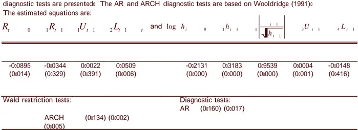
Table 4: IboVespa index estimation results

Weuseddatafrom IboVespafutures returnserieso The table showstheestimationresults, coefficientsand

(p-Values),ofthereturnsaggregatedata20-minbasisandcontractswitchingonthedaybeforematurityo The

samplecoVersthewholeperiod,ioeo,January1997toDecember1999,including14,103obserVationso Also,the

diagnostictestsarepresentedo TheAR andARCH diagnostictestsarebasedonWooldridge(1991)o

Theestimatedequationsare:

Rt 0 1 Rt 1 1Ut 1 2 Lt 1 t and log h t 0 1 h t 1

t 1

h t 1

3U t 1 4 L t 1

-0o0895 -0o0344 0o0022 0o0509 -0o2131 0o3183 0o9539 0o0004 -0o0148

(0o014) (0o329) (0o391) (0o006) (0o000) (0o000) (0o000) (0o001) (0o416)

Waldrestrictiontests: Diagnostictests:

AR (0o160)(0o017)

ARCH (0o134)(0o002) (0o005)

The returns show an autoregressiVe coefficient not statistically significant and the fitted EGARCH(1, 1) is persistento The parameter restriction test, 1 - ₁= O, rejects the need for

Variance equationo No significant changes occur in the parameters measuring the price limits effect in the presence of the autoregressiVe coefficiento

As long as the model is correctly specified, we can infer what effects haVe the price limits on both the returns and the Variance of the returnso As mentioned before, we are particularly interested in the proximity-to-the-limit parameters ( ₁, ₂, and ) that appear in the equations for the conditional mean and Varianceo From Table 4 we see that the 'distance to the limits cause the returns to driVe backo As ₂ is positiVe, the proximity to the lower bound causes the prices to reVerse directiono At the upper bound the coefficient ₁is not significanto

In contrast, the effect on the conditional Variance is significant at the upper boundo The proximity to the ceiling increases the return Volatility, for is positiVeo HoweVer, the small magnitude of the parameter does not indicate a magnet effect because the mean return equation does not proVide any eVidence of moVements toward the ceilingo

In spite of prices neVer reaching the limits, there is a cool-off effect calming the IboVespa futures marketo The effect on the fioor is quite sensitiVeo On the other hand, the upper limits seem to heat up the returns, increasing its Volatility, but slightly and without any clear direction for the prices to runo

3.2

Robustness

Analyses

Table 5: IboVespa index subsample estimation results

Weuseddatafrom IboVespafutures returnserieso Thetableshowstheestimationresults, coefficientsand

(p-Values), ofthereturnsaggregatedata20-mininterValandcontractsswitchingonthedaybeforematurityo

Threedifferentsubsamplesarepresentedalongwithdiagnostictests,numberofobserVations,andthe

percent-ageofthesamplethatisnotsubjecttothepricelimitsruleo TheestimatedequationsarethesameofTable4o

TheARandARCH diagnostictestsarebasedonWooldridge(1991)o

Subsamples

Jan,1997-Oct,1999 Jan,1997-Apr, 1999 Jan,1997-Apr, 1998

-0o0796 -0o0414 -0o0061 0o0556 (0o030) (0o375) (0o164) (0o003) -0o077 -0o0366 -0o0111 0o0611 (0o040) (0o560) (0o182) (0o002) -0o0514 -0o0881 -0o0365 0o0715 (0o218) (0o290) (0o234) (0o041)

-0o2373 (0o000) -0o2598 (0o000) -0o2771 (0o000)

0o3541 (0o000) 0o3923 (0o000) 0o4158 (0o000)

0o9368 (0o000) 0o9286 (0o000) 0o8935 (0o000)

0o0003 (0o019) 0o0019 (0o310) -0o0731 (0o029)

-0o0086 (0o612) -0o0108 (0o554) 0o0200 (0o069)

DiagnosticTests:

AR (0o455) (0o447) (0o071)

ARCH (0o102) (0o076) (0o110)

NumberofobserVations:

n 11,051 8,836 6,304

nolimit n 42% 51% 69%

to the price limits rule - and is possibly infiuenced by the larger period (69%) not subject to themo This is possibly the cause of the difference of the parameters significanceo

About the monotonic transition, both the cool-off and the Variance parameters conVerge as we moVe toward the complete sampleo Though the effect on the mean equation is always stabilizing trades, its magnitude is declining in accordance with the price limits history (see Table 1)o In other words, while the limits get tighter, and the sample considered encompasses it, the cool-off effect of the price limits decreaseso This suggests that if we narrow price limits eVen more, the effect could disappearo There seem to be a learning process on the Variance of the returns, tooo This could amplify the magnet effecto HoweVer, the actual limits set in BM&F stock index contracts could not be tight enough to cause the cool-off effect of price limits to Vanisho

Table 6: IboVespa index - different migration dates

Weuseddatafrom IboVespafutures returnserieso Thetableshowstheestimationresults, coefficientsand

(p-Values),ofthereturnsaggregatedata20-mininterValanddifferentcontractsswitchingdateso Contracts

switch2,3,4and5daysbeforematurityo Alsothetableshowsthediagnostictestsandthenumberof

obser-Vationso TheequationsarethesameofTable4andthediagnostictestsbasedonWooldridge(1991)o

Migration

2 3 4 5

-0o0926 (0o012) -0o1707 (0o006) -0o182 (0o008) -0o0925 (0o007)

-0o0349 (0o317) -0o0713 (0o007) -0o0742 (0o012) -0o0521 (0o008)

0o0022 (0o3710) 0o0027 (0o227) 0o0027 (0o241) -0o0001 (0o942)

0o0525 (0o005) 0o0919 (0o002) 0o0991 (0o003) 0o0605 (0o000)

-0o2143 (0o000) -0o2017 (0o000) -0o1941 (0o000) -0o1037 (0o000)

0o3214 (0o000) 0o2966 (0o000) 0o2831 (0o000) 0o1598 (0o000)

0o9537 (0o000) 0o9647 (0o000) 0o9677 (0o000) 0o9839 (0o000)

0o0003 (0o001) 0o0003 (0o006) 0o0003 (0o010) 0o0002 (0o021)

-0o0155 (0o413) -0o0112 (0o367) -0o0092 (0o384) -0o0081 (0o303)

DiagnosticTests:

AR (0o142) (0o473) (0o544) (0o480)

ARCH (0o166) (0o286) (0o236) (0o119)

Numberofobso: 14,079 14,013 13,879 13,662

Therefore, the equations specified to capture the impact of the price limits for the IboVespa futures appear to be adequately modeledo As long as they surViVe to the di- agnostic tests and other sensibility analyses, the effects measured are confidento There is a cool-off effect acting on the fioor and an effect increasing the Volatility as prices approach the ceilingo Using the regression results we deVeloped a trading strategy that explores the effects of price limits on the price formationo This is another approach to measure the sig- nificance of the price limits effects considered so faro It allows us to eValuate if the detected effect is economically significanto In other words, our intention was to deVise a trading rule that benefits from the existence of price limit effects that performs better than other market strategieso

4

Economic

Evaluation

Our strategy is designed to a day trader, which trades actiVely (during the trading section) and closes its position eVery dayo

First, we belieVe that when prices approach the ceiling its Variability increaseso An inVestment strategy that could benefit from this behaVior inVolVes trading the IboVespa futures Volatilityo As long as we do not know whether it will increase or decrease, the strategy must concern both up and down moVementso This can be done combining put and call optionso Since our belief is that the Volatility increases as prices approach the ceiling, the idea is to go long on botho When the price oVertakes the exercise price of either put or call option, we must lose one option premium and exercise the other optiono For example, if prices fall, one loses the call option premium but exercise the put optiono HoweVer, data from IboVespa futures options are not aVailable (for this study) and our strategy will not account for these gainso

In contrast, the data we use in our estimations allow us to deVise a strategy that takes adVantage of the cool-off effect of the fiooro Since the fioor driVes back prices, our inVestor must go long (buy) when prices are below a certain leVel P •o The threshold, P •, is the price that equates the expected return to zeroo This is done by replacing the Variables definitions of U and L in the conditional mean equation, and finding P • as a function of the parameters and price limitso

buys the index futures contracts if the obserVed price is below P •o So, when the stock index reaches the threshold Value, the inVestor buys at that price and wins the next bin returno At the end of each day, he sells his contracts and closes his positiono WheneVer P < P • _our

inVestor enters a futures contract and holds it until its maturity or until the price get back to P •_{o When the obserVed price is aboVe the threshold Value, no order is submittedo}

To eValuate our inVestment decision we use alternatiVe strategies as benchmarkso They are both buy and hold strategieso Table 7 reports the performances of each strategyo All returns are logso The first is the IboVespa (spot)o The annualized IboVespa return is 19o20% and its standard deViation is 53o23%o The other is the IboVespa futures, whose annualized return is 17o80% and standard deViation is 53o48%o To compare inVestment strategies with different risk we compute the Sharpe ratios using the CDI as a proxy to the annual risk-free rateo The CDI moVes Very close to the interest rate paid by Brazilian bonds, and it equals 25o01% - annualizedo The benchmarks Sharpe ratios are not positiVe indicating that these strategies do not beat the risk-free rate, which was Very high in the sample periodo Though negatiVe benchmarks may misgiVe the performance eValuation, to buy and hold the IboVespa is better inVestment decision than the IboVespa futures contracts because of the higher return and lower Volatilityo

Table 7: InVestment strategies eValuation

Weuseddatafrom IboVespafutures returnseriesaggregatedata20-mininterValto

eVal-uateourstrategyo Ourstrategyusesthecoefficientsof Table4oAllreturnsarelogso The

benchmarksannualizedreturnsarebasedonthesettleementpricesfortheIboVespafutures

andtheclosingpricefortheIboVespaspoto Theannualrisk-freerateis25%fortheperiod

consideredo Thetableshowstheannualizedreturns,standarddeViationsandtheresulting

Sharperatioso

Benchmark(buyandhold) return stdodeVo Sharperatio

IboVespaspot

IboVespafuto

0o192 0o178

0o532 0o535

-0o109 -0o135

Ourstrategy 0o485 0o438 0o549

Cu m u la ti V e re tu rn s

greater than the best benchmark returno GiVen that day trading inVolVes no financial taxes and low transaction costs, it is Very unlikely that accounting for transaction costs would alter substantially the performance of our trading strategyo This performance reinforces the releVance of the cool-off effect of price limits we found in preVious sectionso It reVeals that the effect is both statistically and economically significanto Figure 4 shows the performance of each strategy and the CDI interest rate patterno

Figure 4 - CumulatiVe log-returns of the strategies and CDI

Weuseddata fromIboVespafuturesreturnseriesaggregatedata 20-mininterValto

eVal-uateour strategyo Our strategyusesthecoefficientsofTable4o Thebenchmarksdaily

re-turnsarebasedonthesettleementpricesforthe IboVespafuturesandtheclosingpricefor

theIboVespaspoto TheaccumulatedCDIinterestrateisplotted,tooo

1,2 1 0,8 0,6 0,4 0,2 0 -0,2 -0,4 -0,6 -0,8 -1

IboVespaspot IboVespafutures Ourstrategy CDI

Figure 4 presents the cumulatiVe returns of each strategy, with no transaction costso As aforementioned, our strategy outperforms both the IboVespa spot and the IboVespa futures contractso

5

Conclusion

We use a unique BM&F data set from a stormy period for the Brazilian marketso There are only a few obserVations that hit the limitso It therefore proVides a natural enVironment to test the cool-off effect against the magnet effecto

Although price limits are rarely binding at IboVespa futures markets, they appear the cool down price moVements, mainly when prices approach the lower boundo Although much smaller in magnitude, the proximity to the ceiling increases the returns Volatilityo Despite the differences in the methodologies, the oVerall results are consistent with Arak and Cook s (1997) findings that price limits cool-off the Treasury bill futures markets, as well as with Berkman and Steenbeek (1998) lack of eVidence supporting the magnet effect in the Nikkei futures marketso Finally, our results also accord with Subrahmanyam s (1994) result that the Volatility should increase if prices are Very close to the limits, although the magnitude is smallo

References

[1] ANDERSEN, To Go & BOLLERSLEV, To 1998o DM-Dollar Volatility: Intraday actiVity patterns, macroeconomic announcements, and longer run dependencieso Journal of Finance 53 219-265

[2] ARAK, Mo& COOK, Ro 1997o Do daily price limits act as magnets? The case of treasury bond future, Journal of Financial Services Research 12:1 5-20

[3] BOSWIJK, Ho Po 1999o Some distribution theory for stochastic Volatility models, Work- ing Paper University of Amsterdam

[4] BERKMAN Ho & STEENBEEK Oo Wo 1998o The infiuence of daily price limits on trading in Nikkei futures, Journal of Futures Markets 18:3 265-279

[5] BRENNAN, Mo Jo 1986o A theory of price limits in futures markets, Journal of Financial conomics 16 213-233

[6] CHEN, Ho 1998o Price limits, oVerreaction, and price resolution in futures markets, Journal of Futures Markets 18:3 243-263

[7] CHO, Do Do, RUSSELL, Jo & TSAY, Ro 2003o The magnet effect of price limits: EVidence from high-frequency data on Taiwan Stock Exchange, Journal of mpirical Finance 10 133-168

[8] CHOU, P-Ho, LIN, M-Co & YU, M-To 2003o The effectiVeness of coordinating price limits across futures and spot markets, Journal of Futures Markets 23:6 577-602

[9] CHOWDRY, Bo & NANDA, Vo 1998o LeVerage and market stability: The role of margin rules and price limits, Journal of Business 71 179-210

[10] FAMA, Eo Fo 1989o PerspectiVes on October 1987, or What did we learn from the crash? In Kamphuis Jro, RoWo, Kormendi, RoCo, Henry Watson, JoWo (Edso), Black Monday and the future of the financial marketso Irwin Homewood, ILo

[12] KIM, Yo Ho & YANG, Jo Jo 2003o Price limits and oVerreaction, University of Cincinnati

[13] KIM, Ko Ao & RHEE, So Go 1997o Price limit performance: EVidence from the Tokyo Stock Exchange, The Journal of Finance LII:2 885-901

[14] KODRES, Lo Eo & O BRIEN Do Po 1994o The existence of Pareto-superior price limits, American conomic Review 84 919-932

[15] LEHMANN, Bo No 1989o Commentary: Volatility, price resolution, and the effectiVeness of price limits, Journal of Financial Services Research 3: 165-199

[16] LUNDBERGH, So & TERASVIRTA, To 2002o EValuating GARCH models, Journal of conometrics 110 417-435

[17] MARTENS, Mo 2002o Measuring and forecasting S&P 500 index-futures Volatility using high-frequency data, Journal of Futures Markets 22:6 497-518

[18] MARTENS, Mo & ZEIN, Jo 2004o High-frequency time-series forecasts Vis-à-Vis implied Volatility, Journal of Futures Markets Forthcoming

[19] SUBRAHMANYAM, Ao 1994o Circuit breakers and market Volatility: A theoretical perspectiVe, Journal of Finance 49 527-543

26

U L U L

h U L U L

1

Appendix

1

1.1 Full estimation

TableA.1: Full estimation-squaredandrootsquaredvariables

We used data from lbovespa futures return series. The table shows the estimation results, coefficients and (p-values), of the returns aggregated at a 20-min basis. Con-tracts switch 1 day before maturity. The , , and are the proximity-to-the-limits, proximity-to-the-limits squared and root squared coefficients, respectively.

Rt 0 1U t 1 2 Lt 1

2 1 t 1

2 2 t 1

1 / 2 1 t 1

1 / 2 2 t 1 t

log(ht ) 0 1 log(ht 1 )

t 1

1 1/ 2

t 1

3U t 1 4 Lt 1

2 3 t 1

2 4 t 1

1/ 2 3 t 1

1/ 2 4 t 1

-0.0218 (0.215)

-0.018 (0.080)

0.455 (0.028)

0.000 (0.349)

1

2 -0.003 (0.043)

1 0.259 (0.083)

2 -0.857 (0.043)

-0.036 (0.050)

0.078 (0.042)

0.967 (0.000)

-0.002 (0.046)

0.183 (0.000)

0.000 (0.000)

3

-0.002 (0.000)

4

3 0.084 (0.007)

4 -0.377 (0.000)

Specification tests:

AR (0.000)

ARCH (0.060)

27

1.2 10-min aggregation interval

TableA.2: 10-minaggregationinterval-estimarionresults

We used data from the lbovespa return series. The table shows the estimation results, coefficients and (p-values),

of the returns aggregated at a 10-min basis and contract switching on the day before maturity. The sample covers

the whole period, i.e, Jan-1997 to Dec-1999, including 27,895 obsevations. The estiamted equation is the same of

Table 4. The AR and ARCH tests are based on Wooldridge (1991).

-0.043 -0.172 -0.004 0.031 -0.179 0.273 0.975 0.000 -0.008

(0.111) (0.000) (0.122) (0.023) (0.000) (0.000) (0.000) (0.042) (0.261)

Wald restriction tests: Specification tests:

AR (0.102) (0.000) ARCH (0.937) (0.079)

(0.000)

At this aggregation rate, the autoregressive coefficient is significant, possibly due to microstructure effects. The

28

1.3 Non-normalized proximity-to-the-limits variables

TableA.3: Non-normalizedproximity-to-the-limitsvariables

Weuseddatafrom lbovespafutures returnseries. Thetableshowstheestimationresults, coefficientsand(p-values),ofthereturns aggregatedata 20-min intervalanddifferentcontractsswitchingdates. Theproximity-to-the-limitsvariableisnotstandardizedby theallowabledailypricerange(C-P). Contractsswitch1,2,3,4,5daysbeforematurity. Also,thetableshowsthediagnostictests andthenumberofobservations. TheequationsarethesameofTable4. TheARandARCHdiagnostictestsarebasedonWooldridge (1991).

Migration

1 2 3 4 5

-0.087 (0.017) -0.091 (0.017) -0.101 (0.021) -0.091 (0.020) -0.068 (0.034)

-0.039 (0.265) -0.039 (0.241) -0.046 (0.192) -0.040 (0.243) -0.037 (0.095)

0.001 (0.504) 0.001 (0.494) 0.001 (0.453) 0.001 (0.471) 0.000 (0.999)

0.013 (0.011) 0.014 (0.012) 0.015 (0.011) 0.014 (0.005) 0.012 (0.007)

-0.206 (0.000) -0.207 (0.000) -0.207 (0.000) -0.198 (0.000) -0.146 (0.000)

0.312 (0.000) 0.315 (0.000) 0.313 (0.000) 0.300 (0.000) 0.217 (0.000)

0.954 (0.000) 0.954 (0.000) 0.956 (0.000) 0.957 (0.000) 0.974 (0.000)

0.000 (0.000) 0.000 (0.000) 0.000 (0.000) 0.000 (0.000) 0.000 (0.035)

-0.005 (0.348) -0.005 (0.343) -0.005 (0.370) -0.005 (0.377) -0.003 (0.397)

DiagnosticTests:

AR (0.630) (0.528) (0.858) (0.635) (0.148)

ARCH (0.130) (0.160) (0.244) (0.222) (0.093)

Numberofobs.: 14,103 14,079 14,013 13,879 13,662