The political economy of exchange rate in Brazil

N

₆₅₆

_{ISSN 0104-8910}

The Political Economy of Exchange Rate in

Brazil

Os artigos publicados são de inteira responsabilidade de seus autores. As opiniões

neles emitidas não exprimem, necessariamente, o ponto de vista da Fundação

The Political Economy of Exchange Rate in

Brazil

Cristina Terra

Graduate School of Economics, Fundação Getulio Vargas

Abstract

This paper reviews part of the political economy literature on exchange rate policy relevant to understanding the political motivations behind the Brazilian exchange rate policy. We shall …rst examine the distributive role of the exchange rate, and the way it unfolds in terms of the desired political goals. We will follow by analyzing exchange policy as indicative of government e¢ciency prior to elections. Finally, we discuss …scal policy from the point of view of political economy, in which the exchange rate re-sults from the macroeconomic equilibrium. Over this review, the Brazilian exchange rate policy is discussed in light of the theories presented.

1

Introduction

Governments de…ne their economic policy by considering both economic con-straints and political considerations. Policy choice is made in two steps. Poli-cymakers face …rstly the de…nition of political economic goals, followed subse-quently by the selection of policies to be adopted to reach those goals. Let us consider the …rst step, that is, the de…nition of the goals of the policymakers’ economic policy. Limited resources and the inter-relation among variables im-pose the priority of certain goals over others. Governments, for example, may not have the administrative or …nancial resources necessary to solve, simultane-ously, problems related to education, health, or housing in large urban centers, forcing some to take precedence over others. Or, in a di¤erent scenario, policy designed for the eradication of poverty may clash with measures of …scal aus-terity intended to …ght the growing pressure of in‡ation. What is, thus, the determining factor for economic policy?

Economic policy may be determined as a response to acute crises in sectors of the economy. This was the case, for example, of the exchange rate crisis in the 1990’s that resulted from abrupt reversals in capital ‡ows. In cases such as this one, economic constraints determine the focus of economic policy: i.e. the need for a solution for the crisis. On the other extreme, during favorable economic periods, in which there are neither imminent economic crises nor mounting vul-nerabilities, it is possible to state that national economic goals are determined, essentially, by political goals. Policy makers will determine policy according to their own leanings, but also with an eye on which economic groups will stand to gain or lose with the policies adopted and the political pressure being exerted, whether on the part of lobbyists or of the ballot.

Secondly, once the main goal of the economic policy has been determined, there follows the task of structuring it to meet overall goals. Returning to the currency crisis of the 90’s, two di¤erent routes presented themselves for solving the crisis, a currency devaluation that would allow for a trade balance adjustment, or alternatively, the adoption of high interest rates that would attract foreign capital while leaving the exchange rate unchanged. The economic policies adopted would each impact economic and social agents in distinct ways. While currency devaluation bene…ts sectors producing tradable goods, it also feeds in‡ation and adversely a¤ects the poorer part of the population with less access to the …nancial markets and their indexation mechanisms. It is clear, thus, that political factors will take on an important role in determining economic policy, even when economic constraints are accounted for.

It is our aim in this paper to analyze political choices such as the ones de-scribed above, pertaining to Brazil’s exchange rate policy over the last 30 years. The period has been marked by alternating periods of currency devaluation poli-cies adopted when the economy reeled from international crises, and periods of exchange rate appreciation, when the focus was …ghting in‡ation.1

In the beginning of our period of analysis, steep currency devaluations re-sulted from the brutal deterioration of the terms of trade due to the two suc-cessive oil crises in the 1970’s, and the foreign debt crisis in the early 1980’s.

The ten years that followed the …rst democratically elected government to take o¢ce in 1985 were marked by soaring in‡ation and a series of economic plans designed to stabilize prices that enclosed, in one way or another, the exchange rate as a nominal anchor, which led in turn, to the valorization of

the real exchange rate. Thus periods of exchange rate appreciation governed by price stabilization policies alternated with periods of sharp devaluation, their undoing.

In‡ation was …nally controlled under the price stabilization plan known as Plano Real, put into e¤ect in 1994. Since then, Brazil’s monetary policy has been centered on maintaining price stability. Brazil went through various currency crises caused by turbulence in the international …nancial markets, such as the Asian crisis of 1997 and the Russian crisis of 1999. The response given to the currency crisis in the 1990’s however, di¤ered sharply from policies adopted in the 1970’s and 80’s. While in the past the Brazilian government imposed steep currency devaluations, in the 90’s the response was of a di¤erent nature, with the adoption of a high interest rate policy that, by attracting foreign capital relieved the pressure on currency devaluation. A concern with keeping in‡ation under control thus became the prevailing goal of economic policy in Brazil.2

Our analysis of the political goals as expressed in the adoption of exchange rate policies is divided in three parts. Firstly, we shall stress the distributive e¤ects of the exchange rate. On the one hand, the more devalued an exchange rate is, the more the tradables sector will bene…t, to the detriment of consumers in general, and those associated to non-tradable goods in particular, lowering their purchasing power. On the other hand, currency devaluation may feed in-‡ation, and in‡ation a¤ects diverse sectors of the economy in di¤erent ways. The setting of the exchange rate is based on con‡icting interests in di¤erent economic groups. The second part analyzes the exchange rate policy as an indi-cator of competency of the policymaker. Finally, we will analyze the economy’s …scal policy. In face of the fact that the …scal policy in‡uences the real ex-change rate’s equilibrium value, we analyze the political determining factors as they a¤ect …scal policy in a democratic regime.

After the introduction, this paper is divided into four sections. In the next section we analyze economic policy as re‡ected in the distributive e¤ect of ex-change rate policies. Section 3 discusses the exex-change rate policy as a tool to signal the government’s competency. Section 4 covers economic policy as ap-plied to …scal policy and its e¤ect on the exchange rate. Finally, section 5, concludes.

2

Distributive e¤ects of the real exchange rate

There are two main channels through which the exchange policy may have distributive e¤ects, a direct and an indirect one. The direct one is due to the fact that the real exchange rate is the relative price of tradable and non-tradable goods, and it will be studied in section 2.1. The indirect channel is due to the fact that the variations in the nominal exchange rate may also exert an in‡uence on the in‡ation rate, especially in an economy with price indexation. This channel is covered in section 2.2.

The analysis carried out in this section is based on the assumption that the government has the tools necessary to in‡uence both the nominal and the real exchange rate at its disposal, which is true, at least in the short run. Let us start by considering then the nominal exchange rate. The nominal exchange rate is no more than the price of the foreign currency. Just as with any price, its value is set according to supply and demand, and the government has at its disposal economic policy tools that a¤ect these variables. The level of interest rates for one, in‡uences the demand for domestic bonds, which in turn has direct incidence on the supply of foreign currency, once foreign investors are forced to buy domestic currency in order to acquire local bonds. The very action of the government buying and selling foreign currency as it adjusts its currency reserves will also a¤ect supply of the foreign currency in the domestic market.

2.1

The tradable versus non-tradable sectors

The real exchange rate is the relative price between tradable and non-tradable goods. A more devalued real exchange rate means a higher relative price of tradable goods, and is therefore associated to gains for tradable goods producers to the detriment of non-commercial goods producers. The con‡ict of interest between these two groups in the economy may be expressed in a simple model describing a small and open economy, in which there are only two types of goods, tradables and non-tradables.3 _{For simplicity let us assume that consumer}

preferences can be described by a Cobb-Douglas utility function:

U(CT; CN) = lnCT + (1 ) lnCN; (1)

where Ci stands for the amount consumed of the good i, for i = T (tradable

good),N (non-tradable good), and is a parameter that indicates the relative weight of the tradable good in the utility function.

Every citizen will select his or her own basket of goods in a manner that maximizes its utility, subject to budget constraint that establishes that the total expenditure with consumption must not exceed his or her income. Each individual’s income is made up of an endowment of tradable or non-tradable goods, depending on the sector that the citizen belongs to. Letting e be the relative price between tradable and non-tradable goods, i.e. the real exchange rate, the budget constraint of citizens in the tradables sector may be described as:

eCT +CN eDT; (2)

while, in the other sector, budget constraint is:

eCT+CN DN; (3)

whereDi is the endowment of goodi, fori=T; N.

We may thus …nd that the maximum utility that may be reached for each type of citizen by substituting his or her optimal consumer choices in the utility function. Thus we obtain the indirect utility function, that represents utility as a function of the real exchange rate. For citizens of the tradables sector, the indirect utility function is written as follows:

VT(e) =hT+ (1 ) lne; (4)

and, for the non-tradables sector,

VN(e) =hN lne; (5)

wherehi ln + (1 ) ln (1 ) + lnDi:

Evidently we see that citizens from the tradables sector prefer higher values of e, i.e., a more depreciated real exchange rate, while citizens of the non-tradables sector are happier the more appreciated the real exchange rate is. In mathematical terms,

@VT(e)

@e >0and

@VN(e)

@e <0 (6)

Let us now consider the choice the government must make in terms of the exchange rate level. For simplicity’s sake we shall not specify which tools the government will use to a¤ect the real exchange rate. We assume that the gov-ernment sets the level of the real exchange rate within certain con…nes set by economic constraints, that is e 2 [e; e].4 _{If the economic policy, in this case}

the real exchange rate, were set by a benevolent policymaker whose single goal is the citizen welfare, he would chose an exchange rate that would maximize the social welfare function, that may be expressed as an average of the citizens utility, that is:

W(e) = VN(e) +VT(e); (7)

where n

1 n, and n is the fraction of citizens in the non-tradables sector

of the economy. It is easy to show that, when the fraction of citizens in the tradables sector is relatively high, the government chooses the most devalued exchange rate, e, and when this fraction is su¢ciently low, policymakers will opt for the most valued the exchange rate,e. Thus the exchange rate chosen by a benevolent policy maker,eb_{, will be:}

eb= efor

1

eotherwise (8)

When taking into consideration political issues in selecting policy, policy-makers stop being merely benevolent and add other elements to the conditions

of maximization. It is evident that the policymaker is still concerned with the well-being of the citizens, as represented in the welfare function. How-ever, other variables may a¤ect the policymaker choices. The policymaker, for example, may be concerned with re-election, and any policy adopted prior to elections may be, under speci…c circumstances, liable to a¤ect the probability of re-election. Alternatively, in a di¤erent scenario, a government without the support of the majority of the House of Representatives may …nd itself forced to create a coalition in order to govern. Further still, certain sectors of the economy may lobby the government, o¤ering advantages for a policy in keeping with their own interests. Such o¤ers may be perfectly legal and conform to democratic rules, such as campaign donations, or conversely, illegal, such as is the case of corruption. Given the distributive nature of the exchange rate, when policymakers adopt speci…c elements of economic policy, they will be essentially a¤ecting the relative weights given to the non-tradable goods sector of the econ-omy. Policymakers thus select the level of the economy’s real exchange rate so as to maximize the function:

W(e) = PVN(e) +VT(e); (9)

where _P is the relative weight of the non-tradable goods sector, taking political factors into consideration.

Bonomo and Terra (2005, 2006) show how lobbying can alter the relative weight of di¤erent sectors of the economy in their objective function when faced with private bene…ts o¤ered in exchange for a policy that is skewed in their favor. Such bene…ts may come under many di¤erent guises. They may amount to campaign donations or the o¤er of future placement in the board of directors of one of the lobbying companies once the term in o¢ce is over, or simply the performance of …nancial transactions in the form of corruption.

Agreements of this nature are customarily kept secret, and are legally un-enforceable. In order to be successful, agreements such as these rely on factors such as mutual trust among the parties involved, and the nature of the social and professional relationships being played out over the long run. Such factors serve to discipline the behavior of the actors involved, since it is not possible to resort to the Courts of Justice. Nevertheless agreements may be broken, either for lack of compliance from one of the parties, or because information leaks to the public, at a high cost to the government’s popularity.

successful agreement and potential costs if the agreements ‡ounder. Whenever policymakers believe deals of this nature carry a su¢ciently high probability of success, they enter into an agreement and elect an economic policy that will bene…t lobbyists.

It is fair to conjecture that lobbyists come from the tradable goods sector, the sector composed mainly of the industrial and agricultural sectors. The industrial sector is the setting of a few oligopolists, which makes it easier to solve the problem of free-riders, and where individual gains are high enough to warrant the e¤ort of lobbying. There are some parts of the agricultural sector, especially those involved with exports, which can be similarly described. This leads us to assume that, in our bare-bones model, the sector of tradable goods organizes itself to lobby the government.

To further simplify we assume that there are two types of policymakers: those close to lobbyists and those distant to lobbyists. We suppose that ‘close’ policymakers are so intimately linked to lobbyists that there is a very low prob-ability of failure and therefore no impediment to making agreements. This class of policymakers will be co-opted by lobbyists. ‘Distant’ policymakers will not enter into agreements with lobbyists because they rate the potential agreements with too low a probability of success. Bonomo and Terra (2006) show that, in this context, dist< cl , where cl is the weight given to the non-tradable

sector by policymakers that are deemed ’close’ to lobbyists and _dist given to policymakers ’distant’ to lobbyists.

We further suppose that dist > 1 and cl 1 . According to the

equation (9), it means that policymakers ’close’ to lobbyists confer very low weights to the non-tradable sector and thus choose the most devalued exchange rate. On the other hand, so called ’distant’ policymakers will bene…t the non-tradable goods sector by choosing a more appreciated exchange rate.

type, they will bene…t the non-tradable goods sector even further in order to stress their distance in relation to lobbyists. As a result we have an exchange rate cycle coming up in the proximity of elections: the exchange rate will, on average, be more appreciated prior to elections than once elections are over.5

There are, in fact, various empirical studies that document this type of electoral cycle in the exchange rate. Frieden et al. (2001) identi…ed an electoral exchange rate cycle in a study based on 26 countries in Latin America and the Caribbean, and Pasço-Fonte and Ghezzi (2001) do the same for Peru. There is similar evidence with respect to Brazil in Bonomo and Terra (1999). In that paper the authors study real exchange rate misalignments in relation to its equilibrium value, with the aim of studying ‡uctuations of the real exchange rate that cannot be explained by purely economic variables. Results show that the misalignments of the real exchange rate may be attributed to two regimes: one that has been overvalued and the other undervalued. Furthermore, the probability of being in an overvalued regime is higher prior to elections, while the there is higher probability of there being an undervalued regime in the periods after elections are held.

Another interesting empirical result is found in Blomberg et al. (2005). The authors show that among Latin American economies those with the largest sector of tradable goods also have a lower probability of maintaining a …xed exchange rate. The result is in keeping with the notion that the tradables sector may organize itself into lobbying groups so as to pressure the government into adopting policies that result in more devalued exchange rates. Given the levels of in‡ation prevalent in the region, the …xed exchange rate regime is invariably associated to the appreciation of its real rate. When the sector is large, there is higher probability that the government is held hostage to its interests. This would result in non-…xed rate regimes, and consequently, regimes less prone to appreciation.

2.2

The trade-o¤ between external competitiveness and

in‡ation …ghting

Another important aspect to be taken into consideration in exchange rate policy is its impact on the rate of in‡ation. As discussed previously, nominal exchange rate devaluation will also result in a real devaluation when the economy presents

price rigidity, i.e., whenever the prices of non-tradable goods do not adjust them-selves instantly and proportionately to variation of the nominal exchange rate. However, nominal devaluation is responsible for raising the price of tradable goods, thereby raising the overall prices in the economy. Further still, if there are indexation mechanisms present in the economy, the price increase will re-sult, at least in part, in an increased in‡ation rate. The impact of nominal devaluation over in‡ation, or ’pass-through’, depends on variables such as the degree of openness of the economy, and existing indexation mechanisms.

The previous section established the distributive character of the exchange rate, due to its relative price function between tradable and non-tradable goods. This section adds yet another element to the analysis, which is the exchange rate’s impact over in‡ation. In‡ation has its own distributive e¤ects. Individuals with access to the …nancial markets have a wider array of indexation mechanisms made available to them. Lower income individuals do not have access to the …nancial markets, and consequently, su¤er greater losses with in‡ation.

The previous model showed that citizens from the non-tradable goods sector prefer an appreciated exchange rate. The cost of in‡ation will reinforce their preference. This section shows that there may be also citizens of the tradables sector who prefer the appreciated exchange rate due to devaluation’s perverse e¤ect over in‡ation.

We may describe this setting with only a few changes to the model of the previous section. In order to capture the e¤ect of exchange rate devaluation over in‡ation we will conduct an analysis in a two-period environment. Citizen preferences correspond to those in equation (1), only in two subsequent periods written as follows:

U( ) = lnCT ;t+ (1 ) lnCN;t+ [ lnCT ;t+1+ (1 ) lnCN;t+1]; (10)

where 2(0;1) is the inter-temporal discount rate.

Budget constraints will now be changed to incorporate the e¤ect of in‡ation over welfare. We suppose that individuals must sell their endowment one period prior to buying their consumption. In a setting that includes in‡ation, the price of their consumption basket may di¤er from the price for which their endowments were sold. Individuals nevertheless have access to an indexation mechanism, albeit incomplete: their income is readjusted according to only a fraction of in‡ation

access to indexation mechanisms. The ’poor’ have a smaller endowment and are less protected from in‡ation than the ’rich’. For the purposes of simplicity, and without impairing our analysis, we may suppose further, that budgets must be met during each period, i.e., there are no income transfers in between the two periods.

Budget constraints of the citizens of the tradable goods sector for each period may be written as follows:

pT ;tCT ;t+pN;tCN;t pT ;t 1Di ti; (11)

where Di is the endowment of an individual i, i = R (rich); P (poor), with DR > DP, t _PP_tt1 is the rate of in‡ation, i.e. the ratio between the price

indices att and t 1. Note that each endowment is priced according to the previous period prices, and i is the fraction of in‡ation according to which

citizen’siincome is readjusted. _i varies between the two groups according to the indexation mechanisms each groups has access to. In particular, we assume that R > P, or, in other words, that wealthier individuals have access to

better mechanisms of indexation.

As for the non-tradable sector citizens, we assume, for simplicity, that they receive the same endowment and have the same level of access to indexation mechanism. Thus, the budget constraint of this group is written as follows:

pT ;tCT ;t+pN;tCN;t pN;t 1DN t: (12)

By the same token, our next step is to calculate the indirect utility function of each citizen following the same procedures adopted in the previous model. This will show us individual preferences with respects to the policy adopted by the government, which, as we will see in the following, will have an e¤ect both on the exchange rate and on in‡ation. The indirect utility function of an individual from the tradables sector, rich or poor, is written as follows:

Vi(et; t) =hi+ (1 ) lnet 1 (1 i) ln t

+ [(1 ) lnet (1 i) ln t+1]; (13)

whereet P_PN;tT ;t is the real exchange rate and

fori=R;P.

Just as with the previous model, equation (13) shows that citizens from the tradable goods sector prefer a more devalued exchange rate. The equation shows, additionally, that the two types of citizens, rich and poor, prefer low in‡ation rates, although in‡ation is more prejudicial for the poor who have lower .

The indirect utility function for individuals from the non-tradable sector is written as:

VN(et; t) =hN lnet 1 (1 ) ln t [ lnet+ (1 ) ln t+1]; (14)

wherehN [ ln + (1 ) ln (1 ) + lnDN] (1 + ):

We put forward two daring hypotheses in order to describe, in a simple way, the government’s in‡uence over the real exchange rate and its impact over in‡ation. Firstly, we suppose that non-tradable prices are under constant in‡ation: PN;t

PN;t 1 = . Secondly, we hypothesize that, for the purposes of this

model, this is a small country and that international prices are …xed, so that the price variation of the tradables sector is proportional to the variation of the nominal exchange rate, i.e., PT ;t

PT ;t 1 =

Et

Et 1, where Et is the nominal exchange

rate.

We know that, given individual preferences, the price index is as follows:

lnPt= lnpT ;t+ (1 ) lnpN;t: (15)

Hence, the two hypotheses above de…ne the following relation between the rate of in‡ation and the exchange rate variation:

t=

et et 1

: (16)

According to equation (16), a devaluation of the real exchange rate over time is associated to higher rates of in‡ation, and the e¤ect of the exchange rate over in‡ation is proportional to the relative weight of the tradable good in the utility function. For the sake of simplicity we assume that government’s only choice variable is the exchange rate in the current period. In order to do that, let us consider the real exchange rate in t 1 a given, and we assume that the real exchange rate for the subsequent period will be equal to one chosen for the current period, i.e.,et=et+1. Once these additional hypotheses are considered,

Vi(et; t) =ki+ [ (1 ) (1 i)] lnet; and (17)

VN(et; t) =kN [ + (1 i)] lnet (18)

whereki hi+ (1 i) lnet 1 (1 + ) (1 i) ln , fori=P;RandkN

hN lnet 1 (1 + ) (1 ) ln :

Even with the cost of in‡ation, citizens from the tradable sector will continue to express a preference for exchange rate devaluation when they see themselves su¢ciently protected from in‡ation, or more precisely, when _i>1 ₁ .

Let us consider the case in which R >1 ₁ > P, i.e., wealthy

indi-viduals have su¢cient means of indexation so that they continue to express a preference for exchange rate devaluation while the poor su¤er so much loss from in‡ation that they persist in their preference for an appreciated exchange rate, even if the exchange rate valorization lowers the relative price of the goods they produce. In this setting, a fraction of the tradable goods sector will prefer an appreciated exchange rate, just as the entire non-tradable goods sector.

The results just described can be summarized by the following inequalities:

@VR(e)

@e >0,

@VP(e)

@e <0 and

@VN(e)

@e <0: (19)

Similarly to what we have done in the previous model, we assume that the government chooses a real exchange rate, within the ranges established by the economic conditions, resulting in a choice in a certain interval: e 2 [e; e].6 This choice is made in such a way as to maximize the government’s utility function that weights each group’s welfare according to political motivations. The objective function of the government can, therefore, be written as:

W(e) = P[VN(e) +VP(e)] +VR(e): (20)

If the relative weight given to citizens in the sector of non-tradable goods and to poor citizens of the tradable goods sector is su¢ciently high, the government will choose the more valued exchange rate, e. Otherwise, the exchange rate chosen will be the most devalued one, e. More speci…cally, we can show that

the exchange rate chosen by politicianP,eP_{, is given by:}7

eP =

(

efor _P (1 ) (1 R)

+ (1 ) (1 )+ (1 P);

eotherwise. (21)

Regarding the factors that determine the relative weight given to each group, let us begin by analyzing the di¤erence between a democratic regime and a dictatorship, to address the important political transition that took place in Brazil in 1985. Democratic governments must please their electorates in order to stay in power, while dictatorships are concerned with those groups that keep them in power. In the case of the Brazilian dictatorship, the regime did not do away with elections altogether, regulating political representation according to its needs. Therefore, the fact that there were elections, in no way imposed limits to the government’s economic choices.

With the transition to democracy, the will of the people certainly began to carry greater weight in the government’s decisions. In order to be reelected, or elect its successors, the government needed the support of the majority of the population. In a closed economy such as Brazil’s, the majority of the people belong to the sector of non-tradable goods. One should expect, therefore, that the democratic regime that followed the unpopular dictatorship would give a bigger weight to the sector of non-tradable goods. For the same reason, during the period of transition to democracy, the weight given to the lower classes should have increased too. In our model, this corresponds to dict< dem. The

result would be a real exchange rate that is more appreciated on average in the democratic regime than in the dictatorship.

2.3

The Brazilian exchange rate policy from the

perspec-tive of its distribuperspec-tive impact

From the beginning of the dictatorship in 1964, to the …rst oil crisis in 1974, the international scenario was very favorable. The exchange rate was kept, on average, appreciated throughout the entire period. At the same time, the wage policy adopted at the time led to real salary loss, and assured the competitive-ness of the exports sector. This scenario, despite exchange rate appreciation, protected the domestic industry, the main bene…ciary of the combined economic policies.

The government did not promote the necessary external adjustment in face of the …rst oil crisis in 1974. Taking advantage of the high international liquidity, it raised the foreign debt to deal with the current account de…cit that was caused by the deterioration of the terms of trade. Bonomo and Terra (2001) argue that government failure to enforce an immediate adjustment of the economy is due to the fact that the military government at the time was concerned with gathering legitimate political support. The Brazilian Army was split in two political trends, a moderate group that included President Ernesto Geisel (1974-1979) to one side, and to the other a hard line group that included his predecessor Emílio Garrastazu Médici (1969-1974), whose term in o¢ce coincided with the so-called economic “miracle”. The search for political legitimacy would have led the President to prioritize in‡ation …ghting to the detriment of balance of payments balance.

There was light exchange rate devaluation after the second oil crisis in 1979, followed later by a sharper devaluation after the foreign debt crisis in 1982. The real exchange rate was devalued at approximately 100% in the period from 1981 to 1985. The devaluation of the real exchange rate carried out based on exchange rate devaluations which, combined with indexation mechanisms, resulted in rising in‡ation rates. In 1985 with the return to democracy the government begins a period of in‡ation …ghting.

From 1985 to 1994 we note the presence of exchange rate cycles that can be explained by a trade-o¤ between in‡ation and devaluation. The decade was marked by various price stabilization plans that, in one way or another, used the exchange rate as a nominal anchor. Since price stabilization did not happen overnight, there was room for exchange rate appreciation. The plans ended up failing and were abandoned, in‡ation returned and the exchange rate was devalued.

Some of these stabilization plan/currency appreciation cycles followed by abandoning plan/devaluation coincided with elections, such as was the case of the very …rst of these plans, the Plano Cruzado. Plano Cruzado was launched the 28th of February 1986, a few month prior to the elections for State Governor and the Legislative branch, set for November of the same year. The plan resulted in an appreciation of the exchange rate prior to elections, and just one week after the elections were held, the government kicked o¤ a series of daily exchange rate devaluations that resulted in a devalued real exchange rate.

uses data from emerging economies and from Iceland to show that, on average, the exchange rate anchor is used in price stabilization plans when they are adopted in the period prior to elections, while, in other periods, a monetary anchor is used. Calvo and Vegh (1999) show that price stabilization plans with exchange rate anchors adopted in Latin America and Israel during the 1990’s led to, overall, an initial period of rising GNP and private consumption. There is, therefore, a noticeable association between price stabilization plans and elections.

Once the great majority of stabilization plans based on an exchange rate anchor failed, we may ask ourselves why, after all, were they adopted so often. Alfaro (2002) puts forward an explanation for the adoption of these short-term plans based on the real appreciated exchange rate’s distributive e¤ects. Bene…ts to the non-tradable goods sector may result in additional support for carrying out the plan, even if only for the short-term.

Another interesting case to be examined in this light is the Fernando Collor administration. From the beginning of his term, Fernando Collor established a radical stabilization plan that, despite resorting to the exchange rate as a nominal anchor, leading to real appreciation, froze the economy’s …nancial as-sets. There was, after all, no control over in‡ation and the exchange rate policy maintained, on average, an appreciated exchange rate during his term in o¢ce. We had as a result, a combination of policies that favored none of the groups identi…ed in the models we introduced. The tradable goods sector was unhappy with the exchange rate appreciation, and even in the non-tradable goods sector those less able to protect themselves from in‡ation su¤ered losses from unbri-dled in‡ation. The president was …nally targeted with an impeachment process under allegations of corruption. This is of course a gross simpli…cation, and there were other factors at play and policies that generated discontent among potential supporters of his government. It was certainly, however, an important factor.

Thus we can interpret the policies adopted as reactions to the international crises of the 1990’s as a sign of this priorization. This was the decade of the Mexican 1994 exchange rate crisis, the Asian crisis of ’97, the Russian crisis of ’98 and the Argentinean crisis of 2001, to cite but a few. This turbulent period in the foreign markets led, to a greater or lesser degree, to a drop in the capital in‡ows to Brazil.

At variance with what took place in the early 1980’s, the response to the exchange rate pressures of the 90’s was a high interest policy that attracted foreign capital. This worked to avoid exchange rate devaluations and preserved price stability. This policy favors the poorest citizens in the economy and the non-tradable sector, to the detriment of wealthier citizens of the tradable goods sector.

3

The exchange rate as an indicator of

compe-tency

In the literature there is also the argument that the exchange rate may be used by the government as an indicator of its competency. The explanation for this is based on the e¤ect an exchange rate devaluation has over the interest rate, and the determining role that the interest rate has in the seigniorage tax collected by the government. The more competent a government is, the less it needs to collect taxes in order to o¤er its services. If, ultimately, currency devaluation corresponds to a form of tax collection by the government, then more competent governments will devalue less. Stein and Streb (2004) and Stein, Streb and Ghezzi (2005) explore this line of reasoning.

We will refrain from describing the complete model for exchange rate as a sign of competency. It is somewhat complex and does not pertain directly to our discussion. We shall introduce just the main lines of the argument to understand its reasoning.

The crucial element in the model is how an exchange rate devaluation a¤ects seigniorage tax collection. Hence, we start by the money demand, which is generated by requiring consumers to hold currency in order to consume. This means consumers are under an additional constraint, as follows:

Mt Ct; (22)

whereMtis the demand for money andCtis total spending with consumption.

accrue from government bonds. From the point of view of the government, this lost income turns into revenue via seigniorage,St:

St=itMt; (23)

since it is saving the interest it would be forced to pay to consumers had they bought bonds instead of holding currency.

The constraint over government resources establishes that government debt variation should be equal to public spending plus the interest paid over current debt, minus the seigniorage revenue:

Dt=itDt 1+

Gt

t

St; (24)

where Dt is government debt in t, Gt is public spending and t a parameter

that represents government competency. The larger the value of t, the more

the government is able to spend for a given quantity of available resources. The parameter is an attempt to show the di¤erent degrees of government e¢ciency in managing public resources in di¤erent administrations. For the problem to be well de…ned, we assume that t2[1; k], for a constantk >1.

We also assume free capital mobility and that bonds issued by di¤erent governments are perfect substitutes, in other words, that when bonds have the same yields, market agents will buy any bond regardless of its national origin. Thus asset price arbitrage will result in equal yields when measured in the same currency. In other words, the uncovered interest parity holds. If we further assume that foreign interest rate is equal to 1, we have that:

1 +it= Et Et 1

: (25)

We have now gathered all the necessary elements to understand how ex-change rate policy can act as an indicator of governmental e¢ciency. Let us take the case in which there are only two periods, with no initial debt, and the government must pay the entire debt incurred by the end of the second period. The governmental budget constraint in period 1 can be written as follows:

D1=

G1

1

i1M1:

By substituting the interest rate parity conditions (25) in the equation above, and rearranging the terms, we have:

G1= 1( D1 e_1M1): (26)

where e_ E1 E0

E0 . Equation (26) shows us that there are three ways that the

government may generate more public spending: being more e¢cient (larger ), by increasing its level of debt, or by generating more seigniorage taxes through exchange rate devaluations.

Let us consider the case in which the public sees simultaneously a high level of public spending and a low level exchange rate devaluation. Noting that the public is not able to observe the other variables at play in governmental choice, they are not, in principle, capable of telling if high government spending results from higher governmental indebtedness or due to increased government e¢ciency. Thus we see the exchange rate policy as an indicator of e¢ciency: a truly e¢cient government may chose a su¢ciently low level exchange rate devaluation for a given level of public spending, in such a way that cannot be replicated by an incompetent government.

Stein and Streb (2004), and Stein, Streb and Ghezzi (2005) show that, in a similar setting, and under speci…c conditions, governments will postpone ex-change rate devaluations until after elections in order to signal greater compe-tency. This generates an exchange rate cycle around election periods in which the exchange rate, on average, is more appreciated prior to elections and more devalued after.

4

The political economy of the …scal policy

The analysis conducted so far is based on the exchange rate policy’s e¤ect on the economy and derived political issues. This section focuses on the political economy of the …scal policy. The exchange rate in this model is no longer the focus of economic policy, and becomes solely the residual e¤ect of the chosen …scal policy.

The national accounts show a relation between …scal policy and real ex-change rate. We know that the national product,Y, can be divided into private consumption, C, investment, I, public expenditures, G, and current account balance,M X:

Y =C+I+G+X M (27)

National accounts, shown in equation (27) are an accounting identity. They are not indicative of variables behavior, nor of the causes of variables behavior, neither of the inter relations among the di¤erent variables. All that the national accounts can tell us is that equation (27) is always veri…ed. On the other hand, there are a number of economic theories that study the determinants of the variables shown in the equation.

We will proceed with a simple theoretical framework, in line with the meth-ods employed so far, so as to focus on policy choices and the inter relations between the variables that a¤ect exchange rate movements. We are interested in the relation between …scal policy and the exchange rate. Let the …scal policy be the variable of choice for the government. The national product, private consumption and investment are taken as given, resulting from choices made in-dependently of the …scal policy selection process. The current account balance will be the adjustment variable. In other words, the result in current account will be such that the identity of the national account holds, given the government’s chosen …scal policy, current product, private consumption and investment levels. The current account balance is an increasing function of the real exchange rate. A depreciated exchange rate, i.e., a higher one, leads to an increase in exports and a drop in imports, resulting in a higher current account balance. Thus, higher levels of government expenditure must be counteracted with a lower current account balance, which, in turn, is associated to an appreciated exchange rate.

case of …scal policy, the literature concentrates on varying preferences relative to …scal policy that are caused by citizens with varying incomes. The basic notion is that wealthy individuals di¤er from lower income brackets because they pay more taxes and thus prefer lower government expenditure. This e¤ect was described by Persson and Tabelini (2000) as reproduced in this paper.

We therefore assume that our model economy has a continuum of citizens indexed byi; i2[0;1], in which each one of them receives a di¤erent endowment of a good, yi. With the sole exception of the quantity of the endowment, all

citizens in this economy are identical, and derive utility from the consumption of a private good, ci, and a public good, g, provided by the government. The

utility function of the consumeriis represented by:

wi=ci+H(g) (28)

whereH(g)is a growing concave function: Hg(g)>0eHgg(g)<0, andgthe

quantity of public goods per capita.

The government collects taxes from citizens transforming them into pub-lic goods at no additional cost. The income tax rate, , is the same for all. Governmental budget constraint is written as:

y=g (29)

wherey R1

0 yidiis the average income in the economy.

Individual consumers, in turn, must also comply with their own budget constraints, which establish that expenditure with consumption should equal their available income:

ci= (1 )yi: (30)

By substituting the budget constraints of the government and its citizens in the citizen utility function, we have the indirect utility function that describes citizen preferences as pertaining to …scal policy. The function is described as:

W(g;yi) = (y g) yi

y +H(g):

The expenditure level most preferred by citizen i,gi_{, is the one that}

maxi-mizes the function (28):

gi =Hg1 yi

Note that individuals with higher income prefer lower levels of government spending.

If the level of public expenditure were set by a benevolent government, the government would choose the one that maximizes the social welfare function of the economy, that, in the case of the economy in question, is written as:

W =

Z 1

0

(y g)yi

y +H(g) di=y g+H(g): (32)

The chosen level of expenditure,g , would therefore be equal to:

g =H_g1(1); (33)

in other words, the preferred level of expenditures on the part of the average income voter.

As is often the case with political economy, the chosen policy does not re‡ect the choice of a benevolent government. On choosing policy the government takes into consideration his political interests, as well as the welfare of its citizens. In this case, the government will act according to its electoral interests.

Let us assume that there are two contenders running for the elections. They announce their electoral platforms, that are expressed in the level of public expenditure after the elections are over. Voters take note of each platform and vote for the candidates of their choice. To simplify the analysis, we will assume none of the candidates’ credibility has been questioned, and that their announced policies will really be put into e¤ect.8

Voters will vote for the candidate that most closely resembles his preferred platform. It is fairly easy to show that, in equilibrium, both candidates will o¤er the same platform, and that it will be the preferred policy of the median voter. The median voter in this economy is the one with respect to whom 50% of the population has a higher income and 50%, a lower income. Hence:

gm=H_g1 ym

y ; (34)

where is the average income of the median voter.

Economies always show some degree of income concentration. There are always a few very wealthy individuals and many individuals with lower incomes.

-20% -10% 0% 10% 20% 30% 40% 50% 60% 70% 80%

1970 1972 1974 1976 1978 1980 1982 1984 1986 1988 1990 1992 1994 1996 1998 2000 2002 2004

Consumption Investment Government Spending Current Account Balance

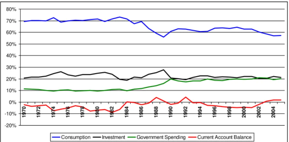
Figure 1: National Accounts, Brazil: 1970-2005

When this occurs, the average income of the economy is higher than the median voter’s income: y > ym.

Given the concavity of the function H(g), the result is that the political contender’s chosen level of expenditures is higher than the socially optimal one. If we add this result to the national account analysis carried out in the beginning of this section, we may conclude that the higher level of expenditure is also associated to an appreciated exchange rate.

Let us consider the facts. With the end of the military dictatorship in the 1980’s and the resulting democratization process, Brazilian politicians become more concerned with elections. According to the model described above, the expected result would be the establishment of policies more in keeping with the median voter, who, in an economy with high income inequality such as Brazil’s, is in a much lower income bracket than the economy’s average income. Among such policies is a more expansionist …scal policy. In fact, from the end of the 1980’s there was a substantial increase in public expenditure, such as can be seen in Figure 1.

With the return to Democracy in 1985, there is a marked change in these variables, pushed by the increase in public expenditures. Public expenditures jump to 20% of the product in 1990, and remain unchanged for the next few years. We can detect two causes for this change. On the one hand democratiza-tion increased electoral concerns among politicians, leading them to implement policies more in keeping with the interests of the median voter. One result was a more expansionist …scal policy. On the other hand, the new constitution that entered into force in 1988 established a variety of compulsory public expendi-tures. This resulted in even heavier public expenditure from that day forward, as shown in …gure 1.

As a compensation for the increase in expenditures, private consumption dropped sharply at …rst, to the level of 56% of the product in 1989, with a small recovery from 1994 onwards. This recovery of private consumption is compensated for an increase in the current account de…cit. As to investments, they remain constant at the 1970’s levels, or: approximately 20% of the GNP, with no more growth spurts.

In short, we note there has been an increase in public expenditures in 1985. Initially this increase was absorbed by the drop in private consumption, but as of 1994, also by the current account de…cits. The increased current account de…cit was consolidated by an appreciated real exchange rate. The post 1994 period shows, therefore, the change predicted by the political economy analysis of public expenditures and their e¤ect over the exchange rate: increasing levels of public expenditure brought about by democratization and leading to current account de…cits, validated by the valuation of the real exchange rate.

5

Conclusion

There is currently in Brazil a debate on whether to adopt the “Chinese Model” and its exchange rate devaluation policy in order to speed up economic growth. What, can we add to this discussion from the perspective of political economy as applied to exchange rate policy? One point all political economy literature share is the identi…cation an appreciated exchange rate with the pref-erences of the median voter. Thus the devalued exchange rate of the Chinese model is an unpopular model. On implementing it, the government should pre-pare itself to lose the support of great part of its electoral basis that will by a¤ected by a reduction in purchasing power.

There remains, too, the issue of how to maintain a depreciated exchange rate. Devaluated exchange rates lead to trade surpluses. According to national accounts identity, such surpluses must be compensated either with an increase in national product, or with a lowering of private consumption, government consumption or of investment. It is hard to imagine that the currency devalua-tion can lead to an increase in nadevalua-tional product that is both substantial and fast enough, without having to resort to a reduction in consumption and investment. Drops in consumption are unpopular while reductions in investment will slow down economic growth. In other words, a devalued exchange rate policy has col-lateral e¤ects that run against the interests of large segments of the population or are damaging to economic growth itself.

Popularity is not an issue for the Chinese government, since it operates as a dictatorship. In a democracy such as Brazil on the other hand, unpopular measures are punished in the voting booths.

References

[1] Aisen, Ari (2002). “Money-Based vs. Exchange-Rate-Based Stabilization: Is there Space for Political Opportunism?” International Monetary Fund Working Paper 04/94:1-30.

[2] Alfaro, Laura (2002). “On the Political Economy of Temporary Stabiliza-tion Programs”,Economics and Politics 14(2): 133-161.

[3] Blomberg, S. Brock, Je¤ry Frieden and Ernesto Stein (2005). “Sustaining Fixed Rates: The Political Economy of Currency Pegs in Latin America”,

[4] Bonomo, Marco and Cristina Terra (1999). “The Political Economy of Ex-change Rate Policy in Brazil: an Empirical Assessment”,Revista Brasileira de Economia 53(4): 411-32.

[5] Bonomo, Marco and Cristina Terra (2001). “The Dilemma of In‡ation vs Balance of Payments: Crawling Pegs in Brazil, 1964-98”, in: J.Frieden and E.Stein (eds.), The Currency Game: Exchange Rate Politics in Latin America (IDB, Washington).

[6] Bonomo, Marco and Cristina Terra (2005). “Elections and Exchange Rate Policy Cycles”,Economics & Politics 17(2): 151-176.

[7] Bonomo, Marco and Cristina Terra (2006). “Political Business Cycles through Lobbying”, mimeo, EPGE/FGV.

[8] Calvo, Guillermo A. and Carlos A.Vegh (1999). “In‡ation Stabilization and BOP Crises in Developing Countries”, NBER Working Paper 6925.

[9] Pascó-Fonte, Alberto and Piero Ghezzi (2001). “Exchange Rates and In-terest Groups in Peru, 1950-1996 em: J.Frieden and E.Stein (eds.), The Currency Game: Exchange Rate Politics in Latin America (IDB, Wash-ington).

[10] Persson, Torsten and Guido Tabellini (2000),Political Economics: Explain-ing Economic Policy, The MIT Press.

[11] Stein, Ernesto H. and Jorge M. Streb (2004). “Elections and the timing of devaluations”,Journal of International Economics 63(1): 119-145.