ESCOLA DE ECONOMIA DE SÃO PAULO
VÍTOR AUGUSTO POSSEBOM
THEORETICAL AND EMPIRICAL ESSAYS ON
MICROECONOMETRICS
VÍTOR AUGUSTO POSSEBOM
THEORETICAL AND EMPIRICAL ESSAYS ON
MICROECONOMETRICS
Dissertação apresentada à Escola de Economia de São Paulo da Fundação Getulio Vargas como requisito para obtenção do título de Mestre em Economia de Empresas
Campo de Conhecimento:
Microeconomia – Modelos Econométricos Orientador: Prof. Dr. Sergio Pinheiro Firpo Co-orientador: Profa. Dra. Cristine Campos de Xavier Pinto
Possebom, Vítor Augusto.
Theoretical and Empirical Essays on Microeconometrics / Vítor Augusto Possebom. - 2016.
60 f.
Orientadores: Sergio Pinheiro Firpo, Cristine Campos de Xavier Pinto Dissertação (mestrado) - Escola de Economia de São Paulo.
1. Microconomia - Modelos econométricos. 2. Testes de hipóteses
estatísticas. 3. Portos e zonas francas - Manaus (AM). 4. Análise de painel. I. Firpo, Sergio Pinheiro. II. Pinto, Cristine Campos de Xavier. III. Dissertação (mestrado) - Escola de Economia de São Paulo. IV. Título.
VÍTOR AUGUSTO POSSEBOM
THEORETICAL AND EMPIRICAL ESSAYS ON
MICROECONOMETRICS
Dissertação apresentada à Escola de Economia de São Paulo da Fundação Getulio Vargas como requisito para obtenção do título de Mestre em Economia de Empresas.
Campo de Conhecimento:
Microeconomia – Modelos Econométricos
Data de Aprovação:
/ /
Banca examinadora:
Prof. Dr. Sergio Pinheiro Firpo (Orientador) Insper
Profa. Dra. Cristine Campos de Xavier Pinto FGV-EESP
Prof. Dr. Bruno Ferman FGV-EESP
Sou grato aos professores, Sergio Firpo, meu orientador, e Cristine Pinto, minha co-orientadora, por tudo que eles me ensinaram não apenas durante o processo de escrever a minha dissertação de mestrado, mas também durante os meus estudos na graduação e na pós-graduação. Eles certamente contribuíram imensamente para minha escolha de carreira e para o economista e econometrista que eu sou hoje.
Eu também sou grato aos professores Bruno Ferman e Ricardo Paes de Barros por serem dois dos primeiros leitores de alguns dos artigos que, talvez, marquem o começo da minha carreira acadêmica. Paes de Barros influenciou mais de uma geração de economistas brasileiros e sou grato por tê-lo encontrado como meu professor na EESP-FGV. Bruno Ferman é muito entusiasmado sobre Economia e contribuiu profundamente para meu conhecimento apesar de nós termos começado a trabalho junto apenas há alguns meses.
Mayra Lora, Enlinson Mattos e Paulo Picchetti também me ensinaram Estatística e Econometria no começo da minha carreira como economista, tendo um papel central na minha decisão de me tornar um pesquisador.
Eu agradeço todos os professores na Escola de Economia de São Paulo por tudo que eles me ensinaram desde 2009. Em particular, Ana Cristina Braga Martes, Vladimir Ponczek, Paulo Furquim, Braz Camargo, André Portela e Paulo Tenani influenciaram minhas decisões profissionais em algum momento. Bernardo Guimarães, que sempre é ávido por economia, também foi um personagem marcante na minha vida profissional, particularmente por ter escrito um interessante livro junto com Carlos Eduardo Gonçalves.
Yoshiaki Nakano sempre foi oquarterbackda Escola de Economia de São Paulo. Sou grato a ele por ter construído um projeto tão incrível, sempre dando suporte aos professores e alunos. Ele também me convenceu a tomar a decisão certa quando eu era um adolescente de 18 anos.
Eu também sou grato a meus professores do ensino básico. Sem eles, não teria sido capaz de aprender tanto durante a minha vida.
Pessoalmente, estarei sempre em dívida com meus pais, Rute Augusto and Francisco Possebom. Eles sempre me oferecerão tudo com amor e me criaram em um ambiente intelectual-mente estimulante. (Todos sabem que Desenvolvimento na Primeira Infância importa. MUITO.) Meu caráter pessoal e meus primeiros passos acadêmicos foram inteiramente influenciados por eles.
Durante o meu mestrado, eu fiz novos amigos e fiquei mais próximo dos antigos. Sou grato a eles pelo suporte acadêmico e, principalmente, emocional. Eles certamente provaram a importância depeer effects. Particularmente, Daniel de Lima, Flávio Riva, João Garcia e Marcela
Mello conquistaram um lugar especial no meu coração. Nós, agora, nos mudamos para diferentes partes do globo, mas espero que sempre estejamos ao lado um dos outros.
Os amigos da minha graduação tem me dado apoio há muito tempo. Nunca esquecerei todos os momentos felizes que tive com eles (e ainda tenho). Um agradecimento muito especial é devido a Natasha Reis e Verena Paiva por todas as nossas extremamente longas e dramáticas conversas. Vocês me mantiveram caminhando durante os últimos dois anos. Sempre desejarei o melhor para vocês.
Meus amigos mais antigos do Bandeirantes estiveram lá apesar da distância física e das minhas frequentes ausências nos raros eventos que reuniam todos em São Paulo. Vocês sempre me ofereceram uma rota de fuga de problemas de matemática para risadas. Vocês se tornaram meu quarto andar.
Também agradeço à FAPESP por financiar minha pesquisa por meio fa bolsa número 2014/23731-3 e à CAPES por fornecer suporte financeiro durante o começo do meu mestrado. Como é fácil provar, ganhar o pão de cada dia é de extrema importância.
I am grateful to professors Sergio Firpo, my supervisor, and Cristine Pinto, my co-supervisor, for everything they have taught me not only during the process of writing my Master’s Thesis, but also during my undergraduate and graduate studies. They surely have contributed immensely to my choice of career and to the economist and econometrician that I am now.
I am also thankful to professors Bruno Ferman and Ricardo Paes de Barros for being two of the first readers of some of the articles that hopefully will mark the start of my academic career. Paes de Barros have greatly influenced more than one generation of Brazilian economists and I am glad to have met him as my professor at EESP-FGV. Bruno Ferman is very enthusiastic about Economics and deeply contributed to my knowledge about it even though we started to work together just a couple of months ago.
Mayra Lora, Enlinson Mattos and Paulo Picchetti have also taught me Statistics and Econometrics at the beginning of my career as an economist, playing a central role in my decision to become a researcher too.
I thank all the professors at Sao Paulo School of Economics for everything they have taught me since 2009. In particular, Ana Cristina Braga Martes, Vladimir Ponczek, Paulo Furquim, Braz Camargo, André Portela and Paulo Tenani influenced my career decisions at some point. Bernardo Guimarães, who is always avid about Economics, was also an important character in my career life, particularly because of an interesting book he wrote with Carlos Eduardo Gonçalves.
Yoshiaki Nakano was the quarterback of São Paulo School of Economics. I am grateful to him for building such an awesome project, always supporting its faculty members and students. He also convinced me to take the right decision when I was a 18 years-old teenager.
I am also thankful to my elementary, middle and high school teachers. Without them, I would not be able to learn so much during my life.
Personally, I am forever in debt to my parents, Rute Augusto and Francisco Possebom. They have provided me everything with love and raised me in an intellectually stimulating environment. (Everyone knows that Early Childhood Development matters. A LOT.) My personal character and my first academic steps were entirely influenced by them.
Lucky is also a member of my family and have always made me company, even when I was explaining to him the First and Second Welfare Theorems. He looked to me so intensely during our lecture sections that I guess he may know more Microeconomics than I will ever know.
me the importance of peer effects. Particularly, Daniel de Lima, Flávio Riva, João Garcia and Marcela Mello conquered a special place in my heart. We now move to different parts of the globe, but I hope we will always be by each other side.
The friends of my undergraduate studies have supported me for a long time now. I will never forget all the happy moments I had with them (and still have). A very special thanks goes to Natasha Reis and Verena Paiva for all our extremely long and dramatic conversations. You kept me walking during the last two years. I will always wish you all the best.
My oldest friends from Bandeirantes were there despite their physical distance or my frequent absences during the rare events when everyone was in São Paulo. You have always provided me a scape route from mathematical problems to laughs. You have become my Floor n. 4.
I am also thankful to FAPESP for funding my research through grant number 2014/23731-3 and to CAPES for supporting me financially during the beginning of my Master’s studies. As it is easy to prove, earning’s one’s daily bread is of paramount importance.
This Master Thesis consists of one theoretical article and one empirical article on the field of Microeconometrics.
The first chapter1, calledSynthetic Control Estimator: A Generalized Inference Procedure and Confidence Sets, contributes to the literature about inference techniques of the Synthetic Control Method. This methodology was proposed to answer questions involving counterfactuals when only one treated unit and a few control units are observed. Although this method was applied in many empirical works, the formal theory behind its inference procedure is still an open question. In order to fulfill this lacuna, we make clear the sufficient hypotheses that guarantee the adequacy of Fisher’s Exact Hypothesis Testing Procedure for panel data, allowing us to test anysharp null hypothesisand, consequently, to propose a new way to estimate Confidence Sets for the Synthetic Control Estimator by inverting a test statistic, the first confidence set when we have access only to finite sample, aggregate level data whose cross-sectional dimension may be larger than its time dimension. Moreover, we analyze the size and the power of the proposed test with a Monte Carlo experiment and find that test statistics that use the synthetic control method outperforms test statistics commonly used in the evaluation literature. We also extend our framework for the cases when we observe more than one outcome of interest (simultaneous hypothesis testing) or more than one treated unit (pooled intervention effect) and when heteroskedasticity is present.
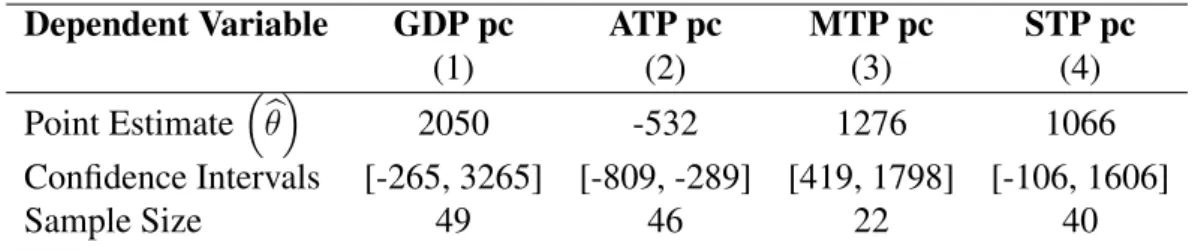
The second chapter, calledFree Economic Area of Manaus: An Impact Evaluation using the Synthetic Control Method, is an empirical article. We apply the synthetic control method for Brazilian city-level data during the 20th Century in order to evaluate the economic impact of the Free Economic Area of Manaus (FEAM). We find that this enterprise zone had positive significant effects on Real GDP per capita and Services Total Production per capita, but it also had negative significant effects on Agriculture Total Production per capita. Our results suggest that this subsidy policy achieve its goal of promoting regional economic growth, even though it may have provoked mis-allocation of resources among economic sectors.
Key-words: Synthetic Control Estimator, Hypothesis Testing, Confidence Sets, Free Economic Area of Manaus, Enterprise Zones.
1 We also thank useful suggestions by Marinho Bertanha, Gabriel Cepaluni, Brigham Frandsen, Dalia Ghanem, Ricardo Masini, Marcela Mello, Áureo de Paula, Cristine Pinto, Edson Severnini and seminar participants at São Paulo School of Economics, the California Econometrics Conference 2015 and the 37thBrazilian Meeting
RESUMO
Esta dissertação de mestrado consiste em um artigo teórico e um artigo empírico no campo da Microeconometria.
O primeiro capítulo contribui para a literatura sobre técnica de inferência do método de controle sintético. Essa metodologia foi proposta para responder a questões envolvendo contrafactuais quando apenas uma unidade tratada e poucas unidades controle são observadas. Apesar de esse método ter sido aplicado em muitos trabalhos empíricos, a teoria formal por trás de seu procedimento de inferência ainda é uma questão em aberto. Para preencher essa lacuna, nós deixamos claras hipóteses suficientes que garantem a validade do Procedimento Exato de Teste de Hipótese de Fisher para dados em painel, permitindo que nós testássemos qualquer hipótese nula do tiposharpe, consequentemente, que nós propuséssemos uma nova forma de estimar conjuntos de confiança para o Estimador de Controle Sintético por meio da inversão de uma estatística de teste, o primeiro conjunto de confiança quando temos acesso apenas a dados agregados cuja dimensão decross-sectionpode ser maior que a dimensão temporal. Ademais, nós analisamos o tamanho e o poder do teste proposto por meio de um experimento de Monte Carlo e encontramos que estatísticas de teste que usam o método de controle sintético apresentam uma performance superior àquela apresentada pelas estatísticas de teste comumente analisadas na literatura de avaliação de impacto. Nós também estendemos nosso procedimento para abarcar os casos em que observamos mais de uma variável de interesse (teste simultâneo de hipótese) ou mais de uma unidade tratada (efeito agregado da intervenção) e quando heterocedasticidade está presente.
O segundo capítulo é um artigo empírico. Nós aplicamos o método de controle sintético a dados municipais brasileiros durante o século 20 com o intuito de avaliar o impacto econômico da Zona Franca de Manaus (ZFM). Nós encontramos que essa zona de empreendimento teve efeitos positivos significantes sobre o PIB Real per capita e sobre a Produção Total per capita do setor de Serviços, mas também teve um efeito negativo e significante sobre a Produção total per capita do setor Agrícola. Nossos resultados sugerem que essa política de subsídio alcançou seu objetivo de promover crescimento econômico regional, apesar de possivelmente ter provocado falhas de alocação de recursos entre setores econômicos.
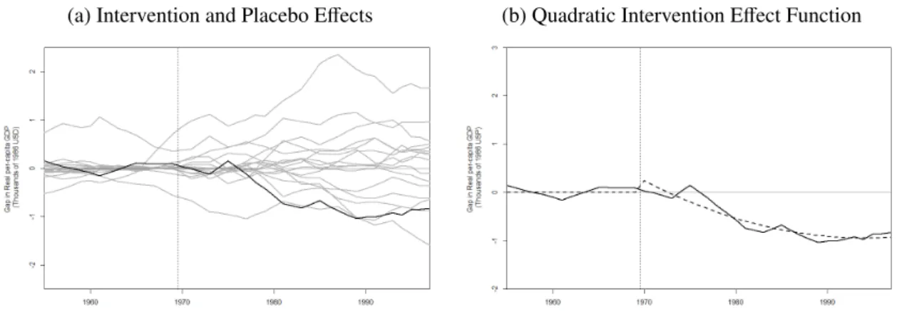
Figura 1 – Estimated Effects using the Synthetic Control Method . . . 40
Figura 2 – 88.9%-Confidence Set for Linear in Time Intervention Effects . . . 40
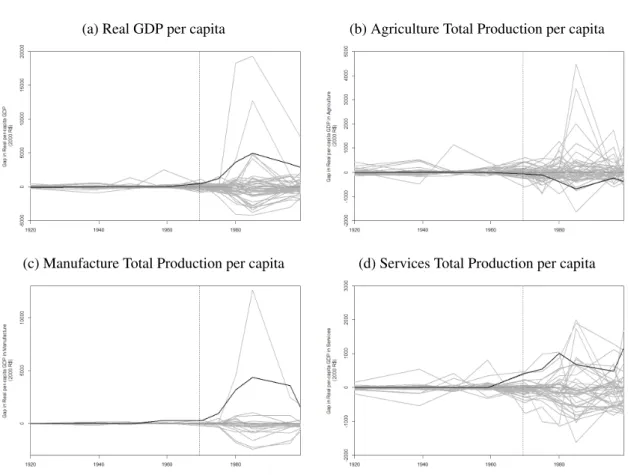
Figura 3 – Estimated Effects using the Synthetic Control Method . . . 56
List of Tables
Tabela 1 – Monte Carlo Experiment’s Rejection Rates . . . 31
Tabela 2 – Monte Carlo Experiment’s Rejection Rates . . . 46
Tabela 3 – Descriptive Statistics . . . 55
1 SYNTHETIC CONTROL ESTIMATOR: A GENERALIZED INFERENCE
PROCEDURE AND CONFIDENCE SETS . . . 16
1.1 Introduction . . . 16
1.2 Synthetic Control Method . . . 19
1.2.1 Synthetic Control Estimator . . . 20
1.2.2 Hypothesis Testing . . . 22
1.2.3 Formalizing and Generalizing the Inference Procedure . . . 23
1.3 Confidence Sets for the Synthetic Control Estimator . . . 26
1.4 Analyzing Size and Power . . . 28
1.5 Extensions to the Inference Procedure . . . 32
1.5.1 Simultaneously Testing Hypotheses about Multiple Outcomes . . . 32
1.5.2 Hypothesis Testing and Confidence Sets with Multiple Treated Units . 34 1.5.3 Hypothesis Testing and Confidence Sets under Heteroskedasticity . . . 37
1.6 Evaluating the Statistical Significance of the Economic Impact of ETA’s Terrorism . . . 38
1.7 Conclusion . . . 41
1.8 Appendices . . . 42
1.8.1 Computing the Observed Test Statistic and its Empirical Distribution . 42 1.8.2 Monte Carlo Experiment’s Complete Set of Results . . . 44
1.8.3 Synthetic Control Method: A Walkthrough . . . 46
2 FREE TRADE ZONE OF MANAUS: AN IMPACT EVALUATION USING THE SYNTHETIC CONTROL METHOD . . . 49
2.1 Introduction . . . 49
2.2 Synthetic Control Estimator . . . 51
2.3 Institutional and Data Description . . . 53
2.4 Results . . . 56
2.5 Conclusion . . . 59
16
1 Synthetic Control Estimator: A Generalized Inference Procedure and Confidence Sets
1.1 Introduction
The Synthetic Control Method was proposed byAbadie e Gardeazabal(2003),
Aba-die, Diamond e Hainmueller (2010) and Abadie, Diamond e Hainmueller (2015) to address
counterfactual questions involving only one treated unit and a few control units. Intuitively, this method constructs a weighted average of control units that is as similar as possible to the treated unit regarding the pre-treatment outcome variable and covariates. For this reason, this weighted average of control units is known as the synthetic control. Although the empirical literature applying the Synthetic Control Method is vast1, this tool’s theoretical foundation is still under development.
Our first contribution to this literature is to formalize the current existing inference pro-cedure proposed byAbadie, Diamond e Hainmueller(2010). Adapting the framework described
byImbens e Rubin(2015) to a panel data context, we clearly state hypotheses that guarantee the
validity of Fisher’s Exact Hypothesis Testing Procedure, a method that compares an observed test statistic to its empirical distribution in order to verify whether there is enough evidence to reject the null hypothesis. Particularly, our framework allow us to test not only the null hypothesis of no effect whatsoever, but also any kind ofsharp null hypothesis, generalizing the current existing inference procedure. The possibility of testing anysharp null hypothesisis relevant in order to approximate the intervention effect function by simpler functions that can be used to predict its future behavior. Most importantly, being able to test more flexible null hypothesis is fundamental to compare the costs and benefits of a policy. For example, one can interpret the intervention effect as the policy’s benefit and test whether it is different than its costs. It also enables the empirical researcher to test theories related to the analyzed phenomenon, particularly the ones that predict some specific kind of intervention effect.
Based on our generalization of the current existing inference procedure, we propose a novel way to estimate Confidence Sets for the Synthetic Control Estimator by inverting a test statistic. We modify the method proposed byImbens e Rubin(2015) to estimate confidence 1 This tool was applied to an extremely diverse set of topics, including, for instance, issues related to terrorism, civil wars and political risk (Abadie e Gardeazabal(2003),Bove, Elia e Smith(2014),Li(2012),Montalvo(2011),
Yu e Wang(2013)), natural resources and disasters (Barone e Mocetti(2014),Cavallo et al.(2013),Coffman e Noy(2011),DuPont e Noy(2012),Mideksa(2013),Sills et al.(2015),Smith(2015)), international finance (Jinjarak, Noy e Zheng(2013),Sanso-Navarro(2011)), education and research policy (Belot e Vandenberghe
(2014),Chan et al.(2014),Hinrichs(2012)), health policy (Bauhoff(2014),Kreif et al.(2015)), economic and trade liberalization (Billmeier e Nannicini(2013),Gathani, Santini e Stoelinga(2013),Hosny(2012)), political reforms (Billmeier e Nannicini(2009),Carrasco, Mello e Duarte(2014),Dhungana(2011)Ribeiro, Stein e Kang
(2013)), labor (Bohn, Lofstrom e Raphael(2014),Calderon(2014)), taxation (Kleven, Landais e Saez(2013),
Souza(2014)), crime (Pinotti(2012b),Pinotti(2012a),Saunders et al.(2014)), social connections (Acemoglu et al.(2013)), and local development (Ando(2015),Gobillon e Magnac(2016),Kirkpatrick e Bennear(2014),Liu
intervals based on Fisher’s Exact Hypothesis Testing Procedure in order to apply it to a panel data framework, using test statistics generated by the Synthetic Control Method. To the best of our knowledge, this is the first work to propose Confidence Sets for the Synthetic Control Estimator when we observe aggregate level data for only one treated unit and a few control units (i.e., small finite samples) in a context whose cross-section dimension may be larger than its time dimension. With our confidence sets, a researcher can quickly show, by using a graph, not only the significance of the estimated intervention effect, but also the precision of this point-estimate. This plot summarizes a large amount of information that is important to measure the strength of qualitative conclusions achieved after an econometric analysis.
Since this generalized inference method and the associated confidence sets can use many different test statistics, we verify, by a Monte Carlo experiment, the size and the power of five test statistics when they are used in this inference procedure. We choose them based on our review of the empirical literature that applies the Synthetic Control Method. More specifically, we compare test statistics that use the Synthetic Control Estimator to test statistics that use simpler methods (e.g.: difference in means and a permuted differences-in-differences test that are commonly used in the evaluation literature) and to the asymptotic inference procedure for the difference-in-differences estimator proposed byConley e Taber(2011). We find that a inference procedure based on a test statistic that uses the Synthetic Control Method performs much better than the ones that do not use this method when we compare their size and power.
We also extend our framework to cover hypothesis testing and confidence set estimation for a pooled effect among few treated units, as a formalization and a generalization of the test proposed byCavallo et al.(2013), and to simultaneously test null hypotheses for different outcome variables. This last extension, that also expands the framework described byAnderson (2008) to a panel data context, is important, for example, to evaluate political reforms (Billmeier
e Nannicini(2009),Billmeier e Nannicini(2013),Carrasco, Mello e Duarte(2014),Jinjarak, Noy
e Zheng(2013),Sanso-Navarro(2011)) that generally affect multiple outcomes variables, such as
income levels and investment. Moreover, we can also interpret each post-intervention time period as a different outcome variable, allowing us to investigate the timing of an intervention effect — a relevant possibility when the empirical researcher aims to uncover short and long term effects. As one last extension, we make some brief comments about cases in which heteroskedasticity is a concern. We stress that choosing a test statistic that is robust to this issue — e.g., the t-test or a modified version of theRMSPEtest statistic — allows us to apply our generalized inference procedure and our confidence sets to empirical problems that present heteroskedasticity.
Capítulo 1. Synthetic Control Estimator: A Generalized Inference Procedure and Confidence Sets 18
conclusion about the size or the sign of the impact of ETA’s terrorism on Basque Country’s GDP per-capita.
Literature Review
Regarding the inference of the Synthetic Control Method, other authors have surely made important previous contributions.Abadie, Diamond e Hainmueller(2010)2are the first authors to propose a inference procedure that consists in estimating p-values through permutation tests andAbadie, Diamond e Hainmueller(2015) suggest a different test statistic for the same procedure. However, they do not make clear the sufficient hypotheses that guarantee that their proposed p-values are valid. One recent advancement in this direction isAndo e Sävje(2013), who discuss the importance of theIdentical and Independent Distributionhypothesis for the inference procedure3and propose two new test statistics that have adequate size and more power when applied to the above mentioned hypothesis test than the ones proposed byAbadie, Diamond
e Hainmueller(2010) andAbadie, Diamond e Hainmueller(2015).
Bauhoff (2014), Calderon (2014) and Severnini (2014) propose a way to apply the
Synthetic Control Estimator to many treated and control units that is similar to a matching estimator for panel data, but none of them discusses its statistical properties in detail. Following a similar but more formal approach,Wong (2015) extends the synthetic control estimator to a cross-sectional setting where individual-level data is available and derives its asymptotic distribution when the number of observed individuals goes to infinity.Wong(2015) also explores the synthetic control estimator when panel data (or repeated cross-sections) are available in two levels: an aggregate level (regions), where treatment is assigned, and an individual level, where outcomes are observed. In this framework, he derives the asymptotic distribution of the synthetic control estimator when the number of individuals in each region goes to infinity. Finally,Cavallo
et al.(2013) andDube e Zipperer(2013) develop different ways to apply the Synthetic Control
Estimator when there are more than one treated unit and propose tests4 that are similar to the ones proposed byAbadie, Diamond e Hainmueller (2010), although they do not address the statistical properties of their inference procedures either.
Gobillon e Magnac(2016), also working on a context with more than one treated unit,
propose a way to compute confidence intervals for their synthetic control estimator based on bootstrapping the point estimate. Although the authors have not clearly stated the assumptions behind their inference procedure either, it requires a large number of treated and control regions in order to be valid and focus exclusively on the time average of the post-intervention effect. Our 2 They also discuss the asymptotic unbiasedness of their method.Kaul et al.(2015) deepen this topic by arguing that using all pre-intervention outcomes as economic predictors might provoke bias by forcing the synthetic control estimator to ignore all other predictor covariates.
3 Our hypotheses are different than the ones advocated byAndo e Sävje(2013). In particular, we do not assume
that units are independent and identically distributed.
approach differs from theirs in two ways: it is valid in small samples and allow the construction of confidence sets for the post-intervention effect as a function of time. Consequently, while their inference procedure allows the empirical researcher to test only constant in time intervention effects, our generalized inference procedure allows the empirical researcher to test any function of time as the intervention effect.
Moreover,Carvalho, Mansini e Medeiros(2015) propose the Artificial Counterfactual Estimator (ArCo), that is similar in purpose to the Synthetic Control Estimator, and derive its asymptotic distribution when the time dimension is large (long panel data sets). However, many of the problems to which the Synthetic Control Method is applied present a cross-section dimension larger than their time dimension, making it impossible to apply the ArCo to them. Wong(2015) also conducts an asymptotic analysis when the pre-intervention period goes to infinity.
Finally, our approach is similar to the wayConley e Taber(2011) estimate confidence intervals for the difference-in-differences estimator in the sense that we also construct confidence sets by inverting a test statistic. However, we differ from them in many aspects. Firstly, while they make a contribution to the difference-in-differences framework, our contribution is inserted in the Synthetic Control literature. Secondly, they assume a functional form for the potential outcomes — imposing that the treatment effect is constant in time — and an arbitrarily large number of control units, while we assume a fixed and (possibly) small number of control units and make no assumptions concerning the potential outcome functional form — i.e., treatment effects can vary in time.
This paper is divided as follows: section 2 explains the Synthetic Control Method as proposed byAbadie e Gardeazabal(2003),Abadie, Diamond e Hainmueller(2010) andAbadie,
Diamond e Hainmueller(2015), and formalizes and generalizes its inference procedure; section
3 proposes a way to estimate Confidence Sets for the Synthetic Control Estimator; section 4 analyzes size and power of different tests statistics employed in this hypothesis test through a Monte Carlo experiment; section 5 develops possible extensions to our framework; section 6 applies our proposed inference procedure to the data set about the Basque Country made available byAbadie, Diamond e Hainmueller (2011) and section 7 concludes. Finally, in the appendices, we didactically explain how to compute the test statistics described in section 2, expand the results of our Monte Carlo Experiment and offer a guide to empirical researchers who wish to employ the synthetic control method in their studies.
1.2 Synthetic Control Method
Capítulo 1. Synthetic Control Estimator: A Generalized Inference Procedure and Confidence Sets 20
Diamond e Hainmueller(2010). Finally, in the third subsection, we clearly state the hypotheses
that guarantees that the current existing inference procedure is valid, generalizing it to test any sharp null hypothesisusing any test statistic.
1.2.1 Synthetic Control Estimator
Suppose that we observe data for (J + 1) ∈ Nregions5 duringT ∈ Ntime periods.
Additionally, assume that there is an intervention6that affects only region 17from periodT0+ 1
to periodT uninterruptedly8, whereT0 ∈(1, T)∩N. Let the scalarYj,tN be the potential outcome
that would be observed for regionjin periodtif there were no intervention forj ∈ {1, ..., J+ 1}
andt ∈ {1, ..., T}. Let the scalarYI
j,tbe the potential outcome that would be observed for region
jin periodtif regionj faced the intervention at periodt. Define
αj,t :=Yj,tI −Yj,tN (1.1)
as the intervention effect (or gap) for regionj in period tand Dj,t as a dummy variable that
assumes value 1 if regionj faces the intervention in periodtand value 0 otherwise. With this
notation, we have that the observed outcome for unitj in periodtis given by
Yj,t :=Yj,tN +αj,tDj,t.
Since only the first region faces the intervention from periodT0+ 1toT, we have that:
Dj,t :=
(
1 ifj = 1andt > T0, 0 otherwise.
We aim to estimate(α1,T0+1, ..., α1,T). SinceY
I
1,t is observable fort > T0, equation (2.1)
guarantees that we only need to estimateYN
1,t to accomplish this goal.
5 We use the word "region"instead of more generic terms, such as "unit", because most synthetic control applications analyze data that are aggregated at the state or country level. We use the termdonor poolto designated the entire group of(J + 1)observed regions.
6 Although the treatment effect literature commonly uses the more generic expression "treated unit", we adopt
the expression "the region that faced an intervention"because it is more common in the comparative politics literature, an area where the synthetic control method is largely applied.
7 In subsection1.5.2, we extend this framework to include the case when multiple units face the same or a similar intervention.
8 Two famous examples of interventions that affect uninterruptedly a region are Proposition 99 — an Tobacco
Control Legislation in California — and the German Reunification, that were studied byAbadie, Diamond e Hainmueller(2010) andAbadie, Diamond e Hainmueller(2015). If the intervention is interrupted (e.g.: ETA’s Terrorism in the Basque Country studied byAbadie e Gardeazabal(2003)), we just have to interpret our treatment differently. Instead of defining the treatment as "region 1 faces an intervention", we define treatment
LetYj := [Yj,1...Yj,T 0]
′be the vector of observed outcomes for regionj ∈ {1, ..., J+1}in the pre-intervention period andXja(K×1)-vector of predictors ofYj.9LetY0 = [Y2...YJ+1] be a(T0×J)-matrix andX0 = [X2...XJ+1]be a(K×J)-matrix.
Since we want to make region 1’s synthetic control as similar as possible to the actual region 1, the Synthetic Control Estimator ofYN
1,t is given, for eacht∈ {1, ..., T}, by
b YN
1,t := J+1 X
j=2 b
wjYj,t, (1.2)
whereWc = [wb2...wbJ+1]′ := Wc(Vb) ∈ RJ is given by the solution to a nested minimization
problem:
c
W(V) :=arg min
W∈W(
X1 −X0W)′V(X1 −X0W) (1.3) whereW :=nW= [w2...wJ+1]′ ∈RJ :wj ≥0for eachj ∈ {2, ..., J + 1} and PJ+1
j=2 wj = 1
o
andVis a diagonal positive semidefinite matrix of dimension(K×K)whose trace equals one. Moreover,
b
V:=argmin
V∈V(
Y1−Y0Wc(V))′(Y1−Y0Wc(V)) (1.4) whereV is the set of diagonal positive semidefinite matrix of dimension(K×K)whose trace equals one.
Intuitively,Wc is a weighting vector that measures the relative importance of each region
in the synthetic control of region 1 andVb measures the relative importance of each one of theK predictors. Consequently, this technique makes the synthetic control of region 1 as similar as possible with the actual region 1 considering theK predictors and the pre-intervention values of the outcome variable when we choose the Euclidean metric (or a reweighed version of it) to evaluate the distance between the observed variables for region 1 and the values predicted by the Synthetic Control Method.10
9 Some lines of matrixXjcan be linear combinations of the variables inYj.
10 Abadie e Gardeazabal(2003),Abadie, Diamond e Hainmueller(2010) andAbadie, Diamond e Hainmueller (2015) propose two other ways to chooseVb. The first and most simple one is to use subjective and previous
knowledge about the relative importance of each predictor. Since one of the advantages of the Synthetic Control Method is to make the choice of comparison groups in comparative case studies more objective, this method of choosingVis discouraged by those authors. Another choice method forVb is to divide the pre-intervention
period in two sub-periods: one training period and one validation period. While data from the training period are used to solve problem (2.2), data for the validation period are used to solve problem (2.3). Intuitively, this technique of cross-validation chooses matrixWc(Vb)to minimize the out-of-sample prediction errors, an
advantage when compared to the method described in the main text. However, the cost of this improvement is the need of a longer pre-intervention period. Moreover, the Stata command made available by those authors also allows the researcher to use a regression-based method in order to compute matrixVb. It basically regress matrix
Y1onX1and imposesvk =|βk|/PK
k′=1|βk′|
Capítulo 1. Synthetic Control Estimator: A Generalized Inference Procedure and Confidence Sets 22
Finally, we define the Synthetic Control Estimator ofα1,t (or the estimated gap) as
b
α1,t :=Y1,t−Yb1N,t (1.5)
for eacht ∈ {1, ..., T}.
1.2.2 Hypothesis Testing
Abadie, Diamond e Hainmueller(2010) propose a inference procedure that
examines whether or not the estimated effect of the actual intervention is large relative to the distribution of the effects estimated for the regions not exposed to the intervention. This is informative inference if under the hypothesis of no intervention effect the estimated effect of the intervention is not expected to be abnormal relative to the distribution of the placebo effects. (p. 497)
In order to do that, they run a permutation test, i.e., they permute which region is assumed to be treated and estimate, for eachj ∈ {2, ..., J + 1}andt ∈ {1, ..., T},αbj,t as described in
subsection1.2.1. Then, they compare the entire vectorαb1 = [αb1,T0+1...αb1,T]
′with the empirical distribution ofαbj = [αbj,T0+1...αbj,T]
′ estimated through the permutation test. If the vector of estimated effects for region 1 is very different (i.e., large in absolute values), they reject the null hypothesis of no effect.
Abadie, Diamond e Hainmueller (2015) note a problem with this approach: |αb1,t|
can be abnormally large when compared to the empirical distribution of|αbj,t| for somet ∈
{T0+ 1, ..., T}, but not for other time periods. In this case, it is not clear at all whether one should
reject the null hypothesis of no effect or not. In order to solve this problem, they recommend to use the empirical distribution of
RM SP Ej :=
PT t=T0+1
Yj,t−Ydj,tN 2
/(T−T0)
PT0
t=1
Yj,t−Ydj,tN 2
/T0
where the acronym RMSPE stands forratio of the mean squared prediction errors. Moreover, they propose to calculate a p-value
p:= PJ+1
j=1 1[RM SP Ej ≥RM SP E1]
J+ 1 , (1.6)
where1[⋄]is the indicator function of event⋄, and reject the null hypothesis of no effect ifpis
less than some pre-specified significance level, such as the traditional value of 0.1.
Although this RMSPE test statistic solve the problem generated by the time dimension of the Synthetic Control Estimator,Abadie, Diamond e Hainmueller(2015) does not state the
sufficient conditions that guarantee the validity of this procedure11nor discuss this test’s size and power. We address the former issue in the next subsection and the latter in section1.4.
1.2.3 Formalizing and Generalizing the Inference Procedure
In this section, we followImbens e Rubin(2015), adapting their framework to a panel data context. We want to formalize and generalize the inference procedure described in subsection
1.2.2. The first hypothesis that we make is thestable unit treatment value assumption(SUTVA):
Assumption 1. The potential outcome vectorsYIj :=Yj,I1...Yj,TI ′ andYNj :=Yj,N1...Yj,TN′for each regionj ∈ {1, ..., J+ 1}do not vary based on whether other regions face the intervention or not (i.e., no spill-over effects in space) and, for each region, there are no different forms or versions of intervention (i.e., single dose treatment), which lead to different potential outcomes (IMBENS; RUBIN,2015, p. 19).
The second assumption concerns the treatment assignment:
Assumption 2. The choice of which unit will be treated (i.e., which region is our region 1) is randomconditional on the choice of the donor pool.12
Although assumption2seems strong, it holds true for many empirical applications of the Synthetic Control Estimator. For example,Barone e Mocetti(2014),Cavallo et al.(2013),
Coffman e Noy(2011) andDuPont e Noy (2012) evaluate the economic effect of large scale
natural disasters, such as earthquakes, hurricanes or volcano eruptions. Although the regions in the globe that frequently faces these disasters are not random, the specific region among them that will be hit by a natural disaster and the timing of this phenomenon is fully random.13Moreover,
Pinotti(2012b) andPinotti(2012a) evaluate the economic and political cost of organized crime in
Italy exploring the increase in Mafia activities after two large earthquakes. Two other examples of the plausibility of assumption2areSmith(2015), who argues that the discovery of large natural resources reserves isas-if-random, andLiu(2015), who argues that the location of land-grand universities in the 19thcentury isas-if-randomtoo.
14
11 Particularly, it is not clear at all what they mean by "the hypothesis of no intervention effect"(ABADIE; DIAMOND; HAINMUELLER,2010, p. 497). Is it a null average effect? Or a null median effect? Or even a
null effect for all units in all time periods? Moreover, asking what these authors mean by "the estimated effect of
the intervention is not expected to be abnormal"(ABADIE; DIAMOND; HAINMUELLER,2010, p. 497) is also a valid question.
12 This assumption is our precise definition of "not expected to be abnormal"in footnote11.
13 In this example, the donor pool contains all countries that frequently faces natural disasters. Conditional on being in the donor pools, being treated (i.e., being hit by a natural disaster in the analyzed time window) is random.
Capítulo 1. Synthetic Control Estimator: A Generalized Inference Procedure and Confidence Sets 24
We also stress that the possibility of choosing the donor pool based on observable covariates implies that assumption2 can be interpreted as imposing only random treatment assignmentconditional on observables, a standard condition in the evaluation literature also known asignorabilityorunconfoundness.
The third assumption is related to how we interpret the potential outcomes: Assumption 3. The potential outcomesYjI :=Yj,I
1...Yj,TI
′
andYjN :=Yj,N
1...Yj,TN
′
for each regionj ∈ {1, ..., J + 1}are fixed buta prioriunknown quantities.15
Implicitly, we assume that we observe therealizationof a random variable for theentire population of interestinstead of a random sample of a larger superpopulation.16
We note that assumptions2and3implies that the units in the donor pool areexchangeable. In reality,exchangeabilityis the weakest assumption that guarantees the valid of our formal and generalized inference procedure, because it is simply based in a permutation test. However, we believe that, although stronger, assumptions2and3makes interpretation easier. In particular, assumption2justifies one of the robustness checks described in appendix1.8.3.
Finally, our null hypothesis is given by asharp null hypothesis:
H0 : Yj,tI =Y N
j,t +fj(t)for each regionj ∈ {1, ..., J+ 1} and time periodt ∈ {1, ..., T},
(1.7) wherefj :{1, ..., T} →Ris a function of time that is specific to each regionj.
Observe that asharp null hypothesisallows us to know all potential outcomes for each region regardless of its treatment assignment. Note also that theexact null hypothesis
H0 : Yj,tI =Y N
j,t for each regionj ∈ {1, ..., J + 1} and time periodt∈ {1, ..., T}, (1.8)
is a particular case of thesharp null hypothesis(1.7) and can be interpreted as an hypothesis of no intervention effect whatsoever. We underscore that equation (1.8) is our precise definition of "no intervention effect"in footnote11.17 We also note that, under assumptions1-3and the null hypothesis (1.8), the p-value in equation (1.6) is valid and known asFisher’s Exact p-Value, afterFisher(1971). In this sense, our inference procedure with the sharp null hypothesisis a generalization of the inference procedure proposed byAbadie, Diamond e Hainmueller(2015). Although thesharp null hypothesis(1.7) is theoretically interesting due to its generality, we almost never have a meaningful null hypothesis that is precise enough to specify individual 15 As a consequence of this assumption, all the randomness of our problem come from the treatment assignment. 16 SeeImbens e Rubin(2015) for details regarding this interpretation.
17 Observe that theexact null hypothesis(1.8) is stronger than assuming that thetypical(mean or median) effect
intervention effects for each observed region. For this reason, we can simply assume a simpler sharp null hypothesis18:
H0 : Yj,tI =Y N
j,t +f(t)for each regionj ∈ {1, ..., J + 1} and time periodt∈ {1, ..., T},
(1.9) wheref :{1, ..., T} →R.
After formally stating conditions that guarantee the validity of the inference procedure proposed by Abadie, Diamond e Hainmueller (2010) and Abadie, Diamond e Hainmueller (2015), we generalize it to other test statistics and to anysharp null hypothesis. We, again, follow
Imbens e Rubin(2015).
We define a test statisticθf as a known positive real-valued functionθf(ι, τ,Y,X, f)of:
1. the vectorι:= [ι1...ιJ+1]′ ∈RJ+1of treatment assignment, whereιj = 1if regionj faces
the intervention at some moment in time and zero otherwise; 2. τ := [τ1...τT]′ ∈RT, whereτt= 1ift > T0 and zero otherwise;
3. the matrix
Y:=
YI
1,1ι1τ1+Y1N,1(1−ι1τ1) ... Y1I,Tι1τT+Y1N,T(1−ι1τT) . ..
YI
J+1,1ιJ+1τ1+YJN+1,1(1−ιJ+1τ1) ... YJI+1,TιJ+1τT+YJN+1,T(1−ιJ+1τT)
of observed outcomes;
4. the matrixX:= [X1X0]of predictor variables;
5. the intervention effect functionf : {1, ..., T} → Rgiven by the sharp null hypothesis
(1.9).
The observed test statistic is given byθobs
f :=θ(e1, τ,Y,X, f)and, under assumptions
1-3and thesharp null hypothesis(1.9), we can estimate the entire empirical distribution ofθf
by permuting which region faces the intervention, i.e., by estimatingθf(ej, τ,Y,X, f)for each
j ∈ {1, ..., J+ 1}, whereej is thej-th canonical vector ofRJ+1.19 We reject the sharp null
hypothesis(1.9) if
pθf :=
PJ+1 j=1 1
θ(ej, τ,Y,X, f)≥θobsf
J + 1 ≤γ (1.10)
Capítulo 1. Synthetic Control Estimator: A Generalized Inference Procedure and Confidence Sets 26
γis some pre-specified significance level20Note that rejecting the null hypothesis implies that there is some region with a non-zero effect for some time period. Moreover, observe thatRMSPE and any linear combination of the absolute estimated synthetic control gaps are test statistics according to this definition. Consequently, the hypothesis tests proposed byAbadie, Diamond e
Hainmueller(2010) andAbadie, Diamond e Hainmueller(2015) are inserted in this framework.21
Regarding the choice of functionf, there are many interesting options for a empirical
re-searcher. For example, after estimating the intervention effect function(αb1,1, ...,αb1,T0+1, ...,αb1,T), the researcher may want to fit a linear, a quadratic or a exponential function to the estimated points associated with the post-intervention period. He or she can then test whether this fitted function is rejected or not according to our inference procedure. This possibility is useful in order to predict, in a very simple way, the future behavior of the intervention effect function.
Another and possibly the most interesting option for functionf is related to cost-benefit
analysis. If the intervention cost and its benefit are in the same unit of measurement, function
f can be the intervention cost as a function of time and our inference procedure allows the
researcher to test whether the intervention effect is different than its costs.
Moreover, functionf can be chosen in order to test a theory that predicts a specific form
for the intervention effect. For example, imagine that a researcher is interested in analyzing the economic impact of natural disasters (Barone e Mocetti(2014),Cavallo et al.(2013),Coffman e Noy(2011),DuPont e Noy(2012)). Theory predicts three different possible intervention effects in this case: (i) GDP initially increases due to the aid effect and, then, decreases back to its potential level; (ii) GDP initially decreases due to the destruction effect and, then, increases back to its potential level; and (iii) GDP decreases permanently due to a reduction in its potential level. The researcher can choose a inverted U-shaped functionfi, a U-shaped functionfiiand a
decreasing functionfiiiand apply our inference procedure to each one of those threesharp null
hypothesesin order to test which theoretical prediction is not rejected by the data.
1.3 Confidence Sets for the Synthetic Control Estimator
Following the inference procedure described at the end of subsection1.2.3, we can test many different types ofsharp null hypothesis. Consequently, we can invert the test statistic to estimate confidence sets for the treatment effect function. Formally, under assumptions1-3, we 20 Yates(1984) stresses thatγshould be chosen carefully and always clearly reported since the discreteness of data (the number of regions is always a finite, usually small, natural number) may preclude the choice of the usual significance levels of 10% or 5%.
21 In section1.4, we analyze five different test statistics that were previously proposed in the synthetic control
literature in order to select the ones that have power against an alternative hypothesis similar toHa: Y1I,t=
YN
can construct aγ-confidence set in the spaceR{1,...,T}as
CSγ,θ :=
f ∈R{1,...,T} :p
θf > γ . (1.11)
Note that it is easy to interpretCSγ,θ: it contains all intervention effect functions whose
associated sharp null hypotheses are not rejected by the inference procedure described in subsection1.2.3.
However, although theoretically possible to define such a general confidence set, null hypothesis (1.9) might be too general for practical reasons since the spaceR{1,...,T}is too large to be informative and estimating such a confidence set would be computationally infeasible. For these reasons, we propose to assume the following null hypothesis:
H0 : Yj,tI =Y N
j,t +c×1(t ≥T0+ 1) (1.12)
for each regionj ∈ {1, ..., J + 1}and time periodt ∈ {1, ..., T}, wherec∈R. Intuitively, we
assume that there is a constant (in space and in time) intervention effect. Note that we can apply the inference procedure described in subsection1.2.3to any c∈ R, estimating the empirical
distribution ofθc. Under assumptions1-3, we can then construct aγ-confidence interval for the
constant intervention effect as
CIγ,θ :={c∈R:pθc > γ} ⊆CSγ,θ (1.13)
whereγ ∈(0,1)⊂R. It is easy to interpretCIγ,θ: it contains all constant in time intervention
effects whose associated sharp null hypotheses are not rejected by the inference procedure described in subsection1.2.3.
We can easily extend (1.12) and (1.13) to a linear in time intervention effect (with intercept equal to zero). Assume
H0 : Yj,tI =Yj,tN +ec×(t−T0)×1(t≥T0 + 1) (1.14)
for each regionj ∈ {1, ..., J + 1}and time periodt ∈ {1, ..., T}, whereec∈R. Intuitively, we
assume that there is a constant in space, but linear in time intervention effect (with intercept equal to zero). Note that we can apply the inference procedure described in subsection1.2.3 to anyec∈R, estimating the empirical distribution ofθec. Under assumptions1-3, we can then
construct aγ-confidence set for the linear intervention effect as
f CSγ,θ:=
(
f ∈R{1,...,T} : f(t) = ce×(t−T0)×1(t≥T
0+ 1)
andpθec > γ
)
Capítulo 1. Synthetic Control Estimator: A Generalized Inference Procedure and Confidence Sets 28
whereγ ∈(0,1)⊂R. It is also easy to interpretCRgγ,θ: it contains all linear in time intervention
effects (with intercept equal to zero) whose associatedsharp null hypothesesare not rejected by the inference procedure described in subsection1.2.3.
We also note that extending our confidence intervals to two-parameter functions (e.g.: quadratic, exponential and logarithmic functions) is theoretically straightforward as equation (1.11) makes clear. However, since we believe that computationally estimating such confidence sets would be extremely time consuming for the practitioner, we opted for restricting our main examples to one-parameter functions (equations (1.13) and (1.15)).
Finally, we highlight that confidence sets (1.13) and (1.15) summarizes a large amount of relevant information since they not only show the statistical significance of the estimated intervention effect, but also provide a measure of the precision of the point-estimate, indicating the strength of qualitative conclusions. Section1.6exemplifies the communication efficacy of this graphical device.
At the authors’ webpage (<https://goo.gl/4Jvd2W>), there is a R function that imple-ments confidence sets (1.13) and (1.15) using theRMSPEas a test statistic.
1.4 Analyzing Size and Power
In this section, we analyze the size and the power of five different test statistics when they are applied to the inference procedure described in subsection1.2.3.22 In order to do that, we assume seven different intervention effects, simulate 5,000 data sets for each intervention effect through a Monte Carlo experiment and, for each data set, we test, at the 10% significance level, the exact null hypothesis(equation (1.8)), following the mentioned inference procedure and using each test statistic. Firstly, we explain how we generated our data sets. Then, we describe our five test statistics. Finally, at the end of this section, we present and discuss the results of our Monte Carlo experiment.
The first step in our Monte Carlo experiment is to decide the values of the parameters:
J+ 1(number of regions),T (number of time periods),T0 (number of pre-intervention time
periods) andK(number of predictors). In our review of the empirical literature, we found that typical values of these parameters are, approximately,T = 25,T0 = 15andK = 10(nine control
variables and the pre-intervention average of the outcome variable). We also setJ+ 1 = 20(one
treated region and nineteen control regions). Our data generating process follows equation (5)
ofAbadie, Diamond e Hainmueller(2010) and is different from the one used byAndo e Sävje
(2013):
YN
j,t+1 =δtYj,tN +βt+1Zj,t+1+uj,t+1
Zj,t+1 =κtYN
j,t +πtZj,t+vj,t+1
for eachj ∈ {1, ..., J+ 1}and t ∈ {0, ..., T −1}, whereZj,t+1 is a(K −1)×1-dimension vector of control variables23. The scalaruj,t+1 and each element of the(K−1)×1-dimension
vectorvj,t+1 are independent random draws from a standard normal distribution. The scalars
δt and κt and each element of βt+1 and πt are independent random draws from a uniform
distribution with lower bound equal to -1 and upper bound equal to+1. We makeZj,0 =vj,0 andYN
j,0 =β0Zj,0+uj,0. Finally, the potential outcome when region 1 faces the intervention in
periodt∈ {1, ..., T}is given by
Y1I,t=Y N
1,t+λ×sd(Y N
1,t|t ≤T0)×(t−T0)×1[t≥T0+ 1], (1.17)
whereλ ∈ {0,0.05,0.1,0.25,0.5,1.0,2.0}is the intervention effect andsd(♣|⋄)is the standard
deviation of variable♣conditional on event⋄. Hence, our alternative hypothesis is that there
is a linear intervention effect only for region 1, implying that our Monte Carlo experiment investigates what are the most powerful test statistics against this alternative hypothesis24.
Note that, in each one of the 35,000 Monte Carlo repetitions, we create an entire popu-lation of regions. Hence, after realizing the values of the potential outcome variables, we can interpret them as fixed buta prioriunknown quantities in accordance to assumption3.25
Now that we have explained our data generating process for our 35,000 Monte Carlo repetitions (5,000 repetitions for each different intervention effect λ), we describe the five
different test statistics that we use to analyze the size and the power of the inference procedure described in subsection1.2.3:
• θ1 :=meanbαej,t
|t ≥T0+ 1
is implicitly suggested byAbadie, Diamond e
Hainmu-eller(2010).
• θ2 :=RM SP Eej is used byAbadie, Diamond e Hainmueller(2015).
• θ3 is the absolute value of the statistic of a t-test that compares the estimated average
post-intervention effect against zero. More precisely,
θ3 :=
αpost/(T−T0)
b
σ/√T−T0
whereαpost :=
PT
t=T0+1αbej,t
(T −T0)
=:θ1 andbσ :=
PT t=T0+1
b
αej,t−αpost
2
(T −T0)
. This test statistic is used byMideksa(2013).
23 Xjis a vector that contains the pre-intervention averages of the control variables and the outcome variable.
24 In a previous version of this text, that circulated under the titleSynthetic Control Estimator: A Walkthrough with Confidence Intervals, we used a constant in time intervention effect. The results of that smaller Monte
Carlo experiment were similar to the ones presented below.
Capítulo 1. Synthetic Control Estimator: A Generalized Inference Procedure and Confidence Sets 30
• θ4 := mean
Yej,t|t≥T0+ 1
−
PT t=T0+1
P
j6=ejYj,t
(T −T0)×J is a simple difference in means
between the treated region and the control regions for the realized outcome variable during the post-intervention period. This test statistic is suggested byImbens e Rubin(2015).
• θ5 is the coefficient of the interaction term in a differences-in-differences model. More
precisely, we estimate the model
Yj,t =η1×1 h
j =eji+η2×1 h
j =eji×1[t≥T0+ 1] +Zj,t×ζ+ξj+µt+εj,t,
whereξj andµtare, respectively, region and time fixed effects, and we makebθ5 =ηb2.
whereej is the region that is assumed to face the intervention in each permutation,mean(♣|⋄)is
the mean of variable♣conditional on event⋄. We construct the empirical distribution of each
test statistic for each Monte Carlo repetition and test the null hypothesis at the 10% significance level. In practice, we reject the null hypothesis if the observed test statistic is one of the two largest values of the empirical distribution of the test statistic.
Note that, although test statistic θ4 and θ5 do not use the synthetic control method,
they are included in our Monte Carlo Experiment for being commonly used in the literature about permutation tests. Since the synthetic control estimator is a time-consuming and computer-demanding methodology, it is important to analyze whether it outperforms much simpler methods that are commonly used in the evaluation literature and that are also adequate in our framework (assumption 1-3). For this same reason, we also report rejection rates for the diff erences-in-differences inference procedure proposed byConley e Taber(2011) (CT)26.
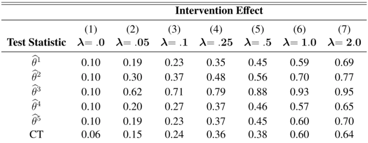
Table1shows the results of our Monte Carlo Experiment. Each cell presents the rejection rate of the permutation test described in subsection1.2.3that uses the test statistic in each row or the rejection rate of the test proposed byConley e Taber(2011) when the true intervention effect is given by the value mentioned in the column’s heading. Consequently, while column (1) presents tests’ sizes27, the columns (2)-(7) present their power.
Analyzing column (1), we note that the five permutation tests of our Monte Carlo Experiment(θ1-θ5)present the correct nominal size as expected by the decision rule of Fisher’s
Exact Inference Procedure. The most interesting result in this column is the conservativeness of the inference procedure proposed by Conley e Taber (2011) (CT), that under-rejects the null hypothesis. This finding can be explained by the fact that, while our sample size is small 26 We estimate the modelYj,t=η1×1
h
j=eji+η2×1 h
j =eji×1[t≥T0+ 1] +Zj,t×ζ+ξj+µt+εj,t, whereξjandµtare, respectively, region and time fixed effects, and test the null hypothesisH0:η2= 0using
the confidence intervals recommend byConley e Taber(2011). Since their inference procedure uses only the control regions in order to estimate the test statistic distribution, the true nominal size of this test is 10.53%. 27 Note that one possible measure of the coverage rate of our confidence set is one minus the rejection rates
Tabela 1 – Monte Carlo Experiment’s Rejection Rates Intervention Effect
(1) (2) (3) (4) (5) (6) (7)
Test Statistic λ=.0 λ=.05 λ=.1 λ=.25 λ=.5 λ=1.0 λ=2.0
b
θ1 0.10 0.19 0.23 0.35 0.45 0.59 0.69
b
θ2 0.10 0.30 0.37 0.48 0.56 0.70 0.77
b
θ3 0.10 0.62 0.71 0.79 0.88 0.93 0.95
b
θ4 0.10 0.20 0.27 0.37 0.46 0.57 0.65
b
θ5 0.10 0.19 0.23 0.37 0.45 0.60 0.70
CT 0.06 0.15 0.24 0.36 0.38 0.60 0.64
Source:Authors’ own elaboration.Notes:Each cell presents the rejection rate of the test associated to each row when the true intervention effect is given by the value λin the columns’ headings. Consequently, while column (1) presents tests’ sizes, the columns (2)-(7) present their power.θb1-θb3
are associated to permutation tests that uses the Synthetic Control Estimator.bθ4-b
θ5are associated
to permutation tests that are frequently used in the evaluation literature. CT is associated with the asymptotic inference procedure proposed byConley e Taber(2011).
(J + 1 = 20), their inference procedure is an asymptotic test based on the number of control regions going to infinity.
Analyzing the other columns, we note that the test statisticRMSPE, proposed byAbadie,
Diamond e Hainmueller(2015)(θ2), is uniformly more powerful than the simple test statistics
(θ4, θ5)that are commonly used in the evaluation literature. This result suggests that, in a context
where we observe only one treated unit, we should use the synthetic control estimator even if the treatment were randomly assigned. We also stress that the hypothesis test based on the statisticRMSPE(θ2)outperforms the test proposed byConley e Taber(2011) (CT) in terms of
power, suggesting that, in a context with few control regions, we should use the synthetic control estimator instead of a differences-in-differences model.
We also underscore that the most powerful test statistic is the t-test,θ3. This result makes
clear the gains of power when the researcher chooses to use the synthetic control estimator instead of a simpler method, such as the difference in means(θ4)or the permuted diff
erences-in-differences test (θ5). We also note that the large power of the t-test have been previously
observed in contexts that are different from ours:Lehmann(1959) looks to a simple test of mean differences,Ibragimov e Muller(2010) analyzes a two-sample test of mean differences where samples’ variances are different from each other, andYoung(2015) focus on a linear regression coefficient.
Finally, we note that the simple average of the absolute post-intervention treatment effect
(θ1), despite using the synthetic control method, is as powerful as the simple test statistics that
are commonly used in the evaluation literature(θ4, θ5). Consequently, we do not recommend to
Capítulo 1. Synthetic Control Estimator: A Generalized Inference Procedure and Confidence Sets 32
stronger suggestion about which test statistic the empirical researcher should use, because, as (EUDEY; KERR; TRUMBO,2010, p. 14) makes clear, this choice is data dependent since the empirical researcher’s goal is to match the test statistic to the meaning of the data. For example, if outliers are extremely important,θ2 may be a better option thanθ3 even though the latter is
more powerful than the former.
In appendix1.8.2, we expand the results of this section to other test statistics.
1.5 Extensions to the Inference Procedure
1.5.1 Simultaneously Testing Hypotheses about Multiple Outcomes
Imbens e Rubin(2015) states that the validity of the procedure described in subsection
1.2.3depends on a prior (i.e., before seeing the data) commitment to a test statistic. Moreover,
Anderson(2008) shows that simultaneously testing hypotheses about a large number of outcomes
can be dangerous, leading to an increase in the number of false rejections.28 Consequently, applying the inference procedure described in subsection1.2.3to simultaneously test hypotheses about multiple outcomes can be misleading, because there is no clear way to choose a test statistic when there are many outcome variables and because our test’s true size may be smaller than its nominal value in this context. After adapting thefamilywise error rate control methodology suggested byAnderson(2008) to our framework, we propose one way to test anysharp null hypothesisfor a large number of outcome variables, preserving the correct test size for each variable of interest.
First, we modify the framework described in section1.2, assuming that there areM ∈N
observed outcome variables —Y1, ...,YM — with their associated potential outcomes. We
change assumptions1-3to:
Assumption 4.The potential outcome vectorsYjm,I :=
h
Yj,m,I1 ...Yj,Tm,Ii′andYjm,N :=
h
Yj,m,N1 ...Yj,Tm,Ni′
for each regionj ∈ {1, ..., J + 1}and each outcome variablem∈ {1, ..., M}do not vary based on whether other regions face the intervention or not (i.e., no spill-over effects in space) and, for each region, there are no different forms or versions of intervention (i.e., single dose treatment), which lead to different potential outcomes.
Assumption 5. The choice of which unit will be treated (i.e., which region is our region 1) is randomconditional on the choice of the donor pool.29
28 List, Shaikh e Xu(2016) argues that false rejections can harm the economy since vast public and private resources can be misguided if agents base decisions on false discoveries. They also point that multiple hypothesis testing is a especially pernicious influence on false positives.
Assumption 6. The potential outcomesYm,Ij :=
h
Yj,m,I1 ...Y m,I j,T
i′
andYjm,N :=
h
Yj,m,N1 ...Y m,N j,T
i′
for each regionj ∈ {1, ..., J+ 1}and each outcome variablem ∈ {1, ..., M}are fixed but a prioriunknown quantities.
Now, our null hypothesis is slightly more complex than the one described in equation (1.9):
H0 : Yj,tm,I =Y m,N
j,t +fm(t) (1.18)
for each regionj ∈ {1, ..., J+ 1}, each time periodt ∈ {1, ..., T}and each outcome variable
m∈ {1, ..., M}, wherefm :{1, ..., T} →Ris a function of time that is specific to each outcome
m. Note that we could index each functionfm by region j, but we opt not to do so because
we almost never have a meaningful null hypothesis that is precise enough to specify individual intervention effects. Observe also that it is important to allow for different functions for each outcome variable because the outcome variables may have different units of measurement or different scales.
Under assumptions4-6and the null hypothesis (1.18), we can, for eachm ∈ {1, ..., M}, calculate an observed test statistic,θobs
fm =θ
m(e
1, τ,Ym,X, fm), and their associated observed
p-value,
pobs θfm :=
PJ+1 j=1 1
θm(e
j, τ,Y,X, fm)≥θfobsm
J + 1
where we choose the order of the indexmto guarantee thatpobs θf1 < p
obs
θf2 < ... < p
obs θfM.
Since this p-value is itself a test statistic, we can estimate, for each outcome m ∈ {1, ..., M}, its empirical distribution by computingpejθ
fm :=
PJ+1 j=1 1
h θm(e
j, τ,Y,X, fm)≥θm,ej
i
J + 1
for each regionej ∈ {1, ..., J+ 1}, where θm,ej := θme
ej, τ,Y
m,X, f m
. Our next step is to calculate pejθ
fm,∗ := min
n pejθ
fm, p
ej
θfm+1, ..., p
e
j θfM
o
for each m ∈ {1, ..., M} and each ej ∈
{1, ..., J + 1}. Then, we estimatepf werθobs ∗ fm :=
PJ+1 j=1 1
h pjθ
fm,∗ ≤p
obs θfm
i
J+ 1 for eachm ∈ {1, ..., M}.
We enforce monotonicity one last time by computingpf werθobs
fm := min
pf werθobs ∗
fm , p
f wer∗ θobs
fm+1
, ..., pf werθobs ∗ fM
for eachm ∈ {1, ..., M}. Finally, for each outcome variablem∈ {1, ..., M}, we reject thesharp null hypothesis(1.18) ifpf werθobs
fm ≤γ
, whereγ is a pre-specified significance level.
It is important to observe that rejecting it for some outcome variablem ∈ {1, ..., M}
implies that there is some region whose intervention effect differs from fm(t)for some time