Investment coordination failures and the confidence channel of fiscal policy

(1)

FUNDAÇÃO GETULIO VARGAS ESCOLA DE ECONOMIA DE SÃO PAULO

MARCEL BERTINI RIBEIRO

INVESTMENT COORDINATION FAILURES AND THE

CONFIDENCE CHANNEL OF FISCAL POLICY

(2)

INVESTMENT COORDINATION FAILURES AND THE

CONFIDENCE CHANNEL OF FISCAL POLICY

Dissertação apresentada à Escola de Economia de São Paulo da Fundação Getulio Vargas, como requisito para obtenção do título de Mestre em Economia

Campo de Conhecimento: Economia Monetária e Fiscal

Orientador: Prof. PhD. Bernardo Gui-marães

(3)

Ribeiro, Marcel Bertini.

Investment Coordination Failures and the Confidence Channel of Fiscal Policy / Marcel Bertini Ribeiro. - 2014.

37 f.

Orientador: Bernardo de Vasconcellos Guimarães

Dissertação (mestrado) - Escola de Economia de São Paulo.

1. Política tributária. 2. Confiança. 3. Concorrência. 4. Investimentos. I. Guimarães, Bernardo de Vasconcellos. II. Dissertação (mestrado) - Escola de Economia de São Paulo. III. Título.

(4)

INVESTMENT COORDINATION FAILURES AND THE

CONFIDENCE CHANNEL OF FISCAL POLICY

Dissertação apresentada à Escola de Economia de São Paulo da Fundação Getulio Vargas, como requisito para obtenção do título de Mestre em Economia

Campo de Conhecimento: Economia Monetária e Fiscal

Orientador: Prof. PhD. Bernardo Gui-marães

Data de Aprovação:

/ /

Banca examinadora:

Prof. PhD. Bernardo Guimarães (Orientador) FGV-EESP

Prof. PhD. Braz Ministério de Camargo FGV-EESP

(5)

RESUMO

Este trabalho desenvolve um novo “canal de Confiança” da política fiscal e caracteriza a política ótima quando esse canal é levado em consideração. Para esse objetivo, utilizamos um modelo estático com (i) concorrência monopolística, (ii) custos de ajustamento fixos para investir, (iii) complementaridade estratégica devido a informação imperfeita com respeito a produtividade agregada, e (iv) bens privados como substitutos imperfeitos de bens privados. Este arcabouço acomoda a possibilidade de falhas de coordenação nos investimentos, mas apresenta um equilíbrio único. Mostramos que a política fiscal tem efeitos importantes na coordenação. Um aumento dos gastos do governo leva a uma maior demanda por bens pri-vados. Mais importante, este também afeta as expectativas de ordem superior com relação a demanda das demais firmas, que amplifica os efeitos do aumento inicial da demanda dev-ido a complementaridade estratégica nas decisões de investimento. Como as demais firmas estão se deparam com uma demanda maior, espera-se que estas invistam mais, que por sua vez, aumenta a demanda individual de cada firma, que aumenta os incentivos a investir. Denominamos isto como o “canal de confiança” da política fiscal. Sob a ameaça de falhas de coordenação, a política fiscal ótima prescreve produzir além do ponto em que o benefí-cio marginal resultante do consumo de bens públicos é igual ao custo marginal desses bens. Este benefício adicional vem do fato de que a política fiscal pode ampliar a coordenação dos investimentos.

(6)

ABSTRACT

This paper proposes a new “confidence channel” of fiscal policy and characterizes the optimal policy taking this channel into account. We develop a static macroeconomic model with (i) monopolistic competition, (ii) fixed adjustment costs for investing, (iii) strategic un-certainty owing to imperfect information about aggregate productivity, and (iv) public goods as imperfect substitutes of private goods. This framework accommodates the possibility of investment coordination failures, but presents a unique equilibrium. We show that fiscal policy has important effects on coordination. An increase in government expenditure leads to higher demand for private goods. Importantly, it also affects higher-order expectations of other firms’ demand, which amplifies the effects of the initial increase in demand, owing to the strategic complementarities in investment decisions. Since other firms are facing higher demand, they are expected to invest more, which raises demand for an individual firm and, consequently, raises its incentives to invest. We dub this the “confidence channel” of fiscal policy. Under the threat of coordination failures, the optimal fiscal policy prescribes produc-ing beyond the point where the marginal benefit from consumproduc-ing public goods equals their marginal cost. The additional benefit comes from fiscal policy enhancing the investment coordination.

(7)

Introduction

Investment slumps are key elements of recessions. Those large and sudden drops in invest-ment are hard to be explained only by productivity shocks. It is argued that firms often choose not to invest because they expect low demand, and low investment levels then corrob-orate low demand expectations. Consumer and investors’ confidence play an important role in this scenario. There is a widespread perception among policy-makers, business community and news-media that government should intervene in economy as to induce “confidence” of households and firms, which would help to stimulate the economy. Nevertheless, as Cochrane (2009) has argued, people “say that we should have a fiscal stimulus to “give people confi-dence,” even if we have neither theory nor evidence that it will work”. Bachmann and Sims (2012) have already made an effort on the latter. Our paper is an attempt at the former and our theoretical results are closely related to their empirical finding with SVAR.

Since Keynes, it is has been argued that investment decisions might be driven by “animal spirits”, i.e., shifts in expectations by no apparent reason. Benhabib and Farmer (1994) and Farmer and Guo (1994) are attempts to revive this idea and Benhabib and Farmer (1999) is a good survey of this literature. A key question there is about whether and when policies interventions could aﬀect demand and lead agents to coordinate in a good equilibrium. This approach yields multiple possible outcomes, hence it comes with the price that these outcomes are not predictable (they are pure shifts in beliefs non related to fundamentals).

We find this approach inappropriate to understand the impacts of government interven-tions. We propose a static model that allows for coordination failures but has a unique equilibrium. Agents investment decisions are strategic complements and expectations are pinned down by fundamentals. It is an standard monopolistic competition model with three additional ingredients: fixed adjustment costs in investment; noisy information about firms productivity; and public goods as imperfect substitutes of private goods. At first glance, they appear not related at all. However, the interaction of them creates a new channel for fiscal policy: the “confidence” channel.

(9)

Introduction 9

varieties in the economy, raising their prices. Therefore, monopolistic competition induces strategic complementarities between firms. Cooper and John (1988) show that strategic complementarities is a necessary condition for multiple equilibria, which may be ranked by welfare criteria. Kiyotaki (1988) gives rise to multiple equilibria introducing increasing re-turns of scale in production in a two period model and Farmer and Guo (1994) in a infinity horizon.1 _{In other words, fixed costs and monopolistic competition can lead to sufficiently}

strong strategic complementarity which yields multiple equilibria.

The second ingredient is imperfect information as firms do not observe the aggregate productivity but receive a noisy signal about it. This assumption creates strategic uncertainty as firms, when deciding whether to invest or not, do not exactly know other firms’ investment decisions. With these informational frictions, we overturn the multiple equilibrium problem as it is possible to find a unique threshold equilibrium. In this equilibrium there is the possibility of coordination failures.

There is a recent growing literature that study the role of noisy information in business cycles.2 _{Our model is specially related to Lorenzoni (2009), Angeletos and La’O (2010)}

and Angeletos and La’O (2013). As in those papers, our model features heterogeneous information about the aggregate productivity.3 _{Unlike their models, our model gives rise to}

ineﬃcient outcomes other than those resulting from monopoly distortions. Guimaraes and Machado (2013) build a model where agents face timing frictions in investment decisions and expected demand plays a key role. As in our model, government interventions can help to mitigate coordination failures, but their framework is specially suitable to answers questions concerning the timing of the interventions. Woodford (2002) uses noisy information about nominal aggregate product and Nimark (2008) noisy information about aggregate marginal cost, and both lead to more inertia in pricing decisions, which is particularly relevant for monetary policy.4

This literature considers the case that Angeletos and Pavan (2004) call weak complemen-tarities, i.e., the equilibrium is unique no matter the structure of information and can be solved by the framework of Morris and Shin (2002). Our paper makes use of strong com-plementarities implied by ﬁxed costs (which induces multiple equilibria in case of

common-1

Other two contributions less related to our paper are: Galí (1996) that argues that when investment goods are also differentiated, the overall demand elasticity depends on the aggregate savings rate in equilibrium which may lead to multiple equilibria if the elasticity of investment goods are higher than consumption goods. Ball and Romer (1991) show that small menu costs in this setup can feature of multiple equilibria.

2

Some papers as Woodford (2002), Nimark (2008), Adam (2007) and others, call this informational setup imperfect common knowledge.

3

In fact, Angeletos and La’O (2010) and Angeletos and La’O (2013) permits a much more general infor-mational structure which agents can also receive signals for other shocks like taste and markup shocks.

4

(10)

Introduction 10

knowledge information about productivity shocks). From a technical point of view, our model builds on the global game literature started with the seminal papers of Carlsson and Damme (1993) and Morris and Shin (1998). Morris and Shin (2003) provides a comprehensive review of this literature.

This paper puts together the ideas from both these literatures to build a model where higher-order expectations are key and multiple outcomes can be achieved as two regimes of a unique threshold equilibrium. In equilibrium, there are regions of intermediate level of productivity (precisely deﬁned later), where coordination failures in investment arise. Firms do not invest because they expected others not to do so, even though it is welfare improving for everyone to invest. In other words, there is a possibility of coordination failures, which means that the private sector cannot provide the desirable level of aggregate demand, as individual choices are not able to deliver the best outcome for the overall economy. Therefore, there is a market failure and thus a reason for government intervention.

We introduce fiscal policy in our model having the government producing a public good that is imperfectly substitute to the other private goods. Hence, our model have important implications to a third strand literature, namely that on the effects of fiscal policy in economic activity. In explicit optimization models, the size of government expenditure multipliers is likely to be low. In the standard real business cycle (RBC) model that happens because, as explained by Aiyagari, Christiano and Eichenbaum (1992) and Baxter and King (1993), there is a negative wealth effect which reduces income and, consequently, brings down consumption and leisure. In New Keynesian (NK) Models, price stickiness generates a second demand channel, but in general its multipliers are still way below one. Moreover, as pointed by Linnemann and Schabert (2003), the effects of fiscal policy depends on monetary policy as the demand channel depends crucially on real interest rate. Building in this insight, Woodford (2011) and Christiano, Eichenbaum and Rebelo (2011) show that when nominal interest rate bind on zero lower bound, effects of government expenditure might be large when the economy is close to the zero lower bound.

The demand channel emphasized by NK models relies on price (or wage) rigidity. There are two drawbacks to this story. First, as argued by Klenow and Malin (2010), evidence on price rigidities at the micro level are not enough to justify large real effects level of policy in macro models. Second, governments widely announce stimulus packages and spending plans. If sticky prices are the key reason for the effects of fiscal policy, why should governments make announcements? Those could only reduce the likelihood that firms are “surprised” by the policy, and thus would lower the policy effects.

(11)

Introduction 11

flexible. The main channel is an expectational one, which justifies the announcements made by fiscal policy authorities. More specifically, depending on the realization of fundamentals, a producer may under-invest in equilibrium, afraid that others might not invest much (which would imply a low demand and thus a low price for her variety). Owing to a technology to produce public goods that are substitute to private sector goods, government can improve agents expectations about their relative price by implementing an expansionary fiscal policy. Such a policy tells firms the demand for their goods will increase. Moreover, firms also expect that other firms will expect more demand. Furthermore, firms have expectations about other firms’ expectations about their increase in demand and so on. We dub this higher-order expectational demand channel (expectations about others’ actions and expectations about others’ expectations about others’ actions and so on ) the “confidence channel”.

This confidence channel yields a productivity threshold, firms decide to pay the fixed cost to invest if productivity is above a certain level. Interestingly, the government expenditure can affect this threshold, changing incentives to invest via this expectational channel. We characterize optimal government interventions showing that under the threat of coordination failures, the government will choose to produce beyond the point where the marginal benefit resulting from the consumption of public goods equals the marginal cost of those goods.

(12)

12

1 Model

In this section, we present a static model of monopolistic competition firms that face fixed costs of investing and informational frictions. Intermediate firms do not observe perfectly the aggregate productivity, which instead receive a noisy signal about this fundamental. This allow us to study the channel of higher-order expectations about other firms’ investment decision and the impacts of fiscal policy in investment decisions through this channel.

1.1 Firms

Final good ﬁrms are perfectly competitive ﬁrms with production function

Y =ωYp

θ₋₁

θ + (1−ω)G θ₋₁

θ

θ θ₋1

(1.1) whereω ∈(0,1) is the share of private goods, Yp ≡

´1

0 y

θ₋1

θ

i di

θ θ₋1

is the amount of private sector good used as input which is a bundle of a continuum of intermediate inputsyi. Gis the

amount of the public good used as input that government gives to this firm for production. Bouakez and Rebei (2007) uses this specification in a RBC model with competitive firms1_,

treating private and public goods as complements. This, for some range of parameters, leads to consumption and government expenditures to be positively correlated as in VAR evidence.2 _{Instead of that, we treat public goods and private goods in the same way. That}

is, the elasticity of substitution, θ > 1, between intermediate private goods yi is equal to

the elasticity of substitution between the private good Yp and the public good G. Hence,

our model incorporate monopolistic competition that implies demand externalities (as we will show later), which make the production decision strategic complements. We prefer this approach as complementarities arise in strategies and not in goods.

1

In their specification, the private goods is single good and here we have a bundle of a continuum of private goods.

2

(13)

Chapter 1. Model 13

The proﬁt of this ﬁrm is3

π =P Y −

ˆ 1

0

piyidi (1.2)

wherepi denotes the price of the intermediate good i and P is the price of the homogeneous

ﬁnal good. Proﬁt maximization implies that the inverse demand for each intermediate variety

i∈[0,1] is :

pi =ωY

1

θy

−1

θ

i P (1.3)

Inserting this equation and using zero proﬁts we ﬁnd the price index: 4

P =ω1−θθ

ˆ 1

0

p1−θ i di

!₁1

−θ

(1.4) Each intermediate goodsyi is produced by a monopolist with the following technology:

yi =Akiα (1.5)

whereAis the productivity that is the same for every ﬁrm; ki denotes the amount of capital

used by ﬁrmi. Firms proﬁt are given by

πi =piyi−PC(ii) (1.6)

where C(·) is a function that denotes the cost of investment, and ii denotes the amount of

investment of ﬁrmi. We assume that there are ﬁxed costs of investing, so thatC(·) takes the form

C(i) =

  

 

i+ψ if i >0 0 if i= 0

This introduce locally increasing returns that may leads to multiple equilibria as monop-olistic competition creates strategic complementarities between investment decisions. Fixed costs are an important feature for investment decisions. Cooper and Haltiwanger (2006) uses panel data with a structural model that incorporates convex and non-convex adjustment costs to explain the investment US data in micro-level. They ﬁnd that the investment rate

3

Since government goods G _{are public goods, firms do not pay for them. This is not essential for our}

results. We prefer this interpretation because the essentiality of public goods which is not true for private goods public supplied.

4

(14)

data has an asymmetric distribution towards positive investment and investment bursts ac-counts for a large share of investment activity. They show that non-convex adjustment costs, as ﬁxed costs are key to explain investment rate moments at plant-level. 5

The law of motion of capital is given by:

ki =k0+ii

where k₀ > 0 denotes the initial level of capital, which is the same across ﬁrms. Since the problem is static, we are assuming no depreciation. We also impose irreversibility of capital, that is,ii ≥0∀i∈[0,1]. This assumption implies that we cannot have an equilibrium which

ﬁrms pay the ﬁxed cost to choose lower capital. 6

Since prices are flexible, intermediate firms have only two interrelated choices: pay the fixed cost or not and if yes, the amount of capital ki. For the rest of the paper we will call

“investing” and “paying the ﬁxed cost for investing” interchangeably.

1.2 Information and Timing

The only source of uncertainty in the model is the aggregate technologyAused by ﬁrms. We assume that all agents do not observeA. Instead, each ﬁrm i receive a noisy signal

xi =A+εi (1.7)

with pdf f that has the following properties: E(εi) = 0 and V ar(εi) = σ2. Hence, ﬁrms

have heterogeneous information that is the main source of the confidence channel. When deciding whether to invest or not, firms have to make forecasts about other firms’ investments decisions. Government, instead, have a general priorg(A) over A.

We define the timing of the economy in three stages. First, government decides the government expenditure G based in his prior g(A). Second, firms receive the signal and decide whether or not to pay the fixed costs that allow changing the level of capital and thus, production. Finally, in last stage, firms choose their desired production given their previous decision and markets clear.

The assumption that government expenditures are decided ﬁrst is in line with the VAR literature on government expenditure eﬀects that followed Blanchard and Perotti (2002). The

5

The other kind of non-convex adjustment costs that Cooper and Haltiwanger (2006) emphasize are: lower idiosyncratic productivity when investing and asymmetries in price of capital when selling or buying capital.

6

(15)

usual assumption is that government expenditure shocks to not respond to output shocks (and other variables introduced in VAR speciﬁcation). The reasoning of this assumption is based on institutional information about ﬁscal policy, which make hard to change quickly government expenditure and taxes in response to the state of economy.

1.3 Households and Government

The economy is populated by a representative household, whose utility function is given by:

U =u(C) (1.8)

whereu′₍

C)>0,u′′₍

C)<0. The budget constraint of households is given by

P C = Π−P T

where Π ≡ ´1

0 πidi is the sum of proﬁts of all ﬁrms and T denotes a real lump-sum tax.

(16)

16

2 Equilibrium

In this section, we follow our timing convention to solve the model. Therefore, we use a backward induction approach. First we find the optimal choices of capital for firms that paid the fixed cost and for the firms which did not. Subsequently, given these optimal choices, we turn to the decision of whether to pay the fixed cost or not.

Inserting 1.3 and 1.5 in profits 1.6 we can find the real profits:

ˆ

πi ≡

πi

P =ω(Ak

α i)

θ₋1

θ _Y 1θ − C(I

i) (2.1)

Lets define{ˆπj, yj}the profits and production of a firm of type j ∈ {I, N}, which stands for

investing and not investing. Anticipating that all firms of the same type will have the same decision, in what follows we are not indexing in ianymore. We first solve the firms problem for a given A and then turn to the decision of paying the fixed cost. 1

The ﬁrst order condition implies the optimal capital choice for typej =I ﬁrms:

k∗

=

"

αω θ−1

θ

!#

θ θ(1−α)+α

A θ₋₁ θ₍₁₋α₎₊α_Y

1

θ₍₁₋α₎₊α (2.2)

We are going to show that the strategic complementarity comes from the fact that the optimal capital decision depends positively on aggregate product Y, which in turn depends on others capital decision. This happens because each ﬁrm faces downward slope demand, which depends on aggregate demand as consequence of monopolistic competition. The type

j =N of firms do not have any choice, i.e, yN =Ak0α. The real profits of each firm type is

ˆ

πI =ωy

θ₋₁ θ

I Y

1

θ −(k∗−k

0)−ψ (2.3)

ˆ

πN =ωy

θ₋1

θ

N Y

1

θ (2.4)

whereyI amount produced by firms which payed fixed cost in first stage is:

yI =

"

αω θ−1

θ

!#θ₍₁₋αθα₎₊α A

θ θ(1−α)+αY

α

θ(1−α)+α (2.5)

1

This procedure is not exactly correct as firms do not observeA _{in this stage. However, as we will make}

clear later, our equilibrium definition is a limiting case whereσ_→_{0. Therefore, we do not need to worry}

(17)

Chapter 2. Equilibrium 17

Given the individual choices of production we can ﬁnd the aggregate product. Lets deﬁne

h as the fraction of ﬁrms who are investing. Hence, the aggregate product is given by:

Y =ωhhyI

θ₋₁

θ + (1−h)y

N

θ₋₁ θ

i

+ (1−ω)Gθ−θ1

θ θ₋1

(2.6) It is clear that since individual productionyI depends on aggregate productY, then equations

2.5 and 2.6 determine the equilibrium aggregate product by solving the fixed point implied by both equations. Due to the fact that the public goodsGenters in the final good production, we cannot find a analytical solution for Y. The following Lemma establish the properties of the aggregate product function, which will play an important role in the unique threshold equilibrium with government expenditure.

Lemma 1. There is a unique Fixed Point solution forY(A, h, G)that is a strictly increasing function of A, h and G.

The proof is in the appendix. The Lemma above shows that the solution for the aggregate production is unique and is increasing in the productivity, in government expenditure in public goods and in the proportion of ﬁrms that are investing. It is important to note that this result is for a given triple (A, h, G). More precisely, if government choose to expend G

and from all firms with productivityA, there is a proportion of hpercent of firms paying the fixed cost, then the aggregate product will be increasing in all its arguments.

We already have enough results to understand how government expenditure affects out-put. Our specification of government expenditures entering in final goods production func-tion may be misinterpreted. Since the work of Barro (1990) that introduces government expenditure in production function, it is usually interpreted as a “government capital” or infrastructure. In other words, government expenditures increases the overall productivity of the economy. This do not happens in our model. It would be the case if the government ex-penditures entered as the other input in the Cobb Douglas intermediate production function instead of in the final good production function.

Instead, our specification treats public goods imperfect substitutes of private goods as intermediate private goods are between themselves. An increase in supply of public goods induce higher demand for the private intermediate goods as final goods firms demands it more as to better balance its inputs. More precisely, an increase in government supply of public goods,G, implies higher aggregate output, Y, by equation 2.6. Moreover, this increases the individual demand for each firm, given by equation 1.3.

(18)

Figure 1 – Investment incentives and Aggregate Demand

to capture the decision made in the second stage, we take the difference the real profits of paying the fixed cost or not, that is:

D(A, h, G)≡πˆI −πˆN =ω

y θ₋₁

θ

I −y

θ₋₁ θ

N

Y 1θ −(k∗−k

0)−ψ (2.7)

if the conditional expectation of the profit difference satisfy E[D(A, h, G)|xi]≥ 0 the firms

choose to pay the fixed cost and invest, and do not pay otherwise. Before characterizing the equilibrium, we first show in the following Lemma the properties of the difference of profits.

Lemma 2. D(A, h, G)≡πˆI(A, h, G)−πˆN(A, h, G) is an increasing function of in A, h and

G.

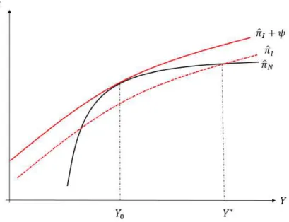
The proof is in the appendix. The Lemma above says that the incentive for paying the fixed cost to invest is higher when productivity is higher. Moreover, the decisions of investing or not are strategic complements, since the higher the proportion of investing firms,h, higher the incentive of an individual firm to pay the fixed cost. Woodford (2002) and Nimark (2008) and others, emphasize the importance of strategic complementarities in price setting. Instead, as our model has flexible prices, our focus is in strategic complementarities via demand linkages in the spirit of Blanchard and Kiyotaki (1987). In order to understand this, the Figure 1 shows the relationship between the investment incentives and the aggregate demand, since it represent profit equations 2.3, 2.4 as function ofY(A, h, G).

(19)

A

A _A¯

No ﬁrm pays ﬁxed costs and investi= 0

Multiple Equilibria

All ﬁrms pay ﬁxed costs and investi=k∗

−k₀

Figure 2 – Multiple Equilibria

non-investing firms to have the same profit, excluding the fixed cost and Y∗_{, including the}

fixed costs, both for a given (A, h, G). As we can see, difference between the profit between investing or not, D(A, h, G), is increasing in Y(A, h, G). That is, more aggregate demand increases individual demand, which implies an increase profits and stronger incentives to invest. The idea is that when firms are investing, they take more advantage of the increasing demand than when they are not. When aggregate demand is sufficiently high, it is enough to firms to have enough additional profit to pay the fixed costs. Since, Y(A, h, G) is increasing in the triple (A, h, G), an increase in any of them has the effect to increase incentives to investment. Therefore, a striking result from this Lemma is that the higher the government expenditure in public goods, higher the incentives for investing. Usually we would expected that higher government expenditure would lead to crowding-out.

The important diﬀerence of our model is that as public goods are imperfect substitutes of private goods and there is monopolistic competition between private sector ﬁrms. An increase in government expenditure lead to higher demand of each intermediate good, which in turn increases incentives to invest. Because public goods are imperfect substitutes of private goods, the increase of supply of these goods, increase the relative price of private goods. In other words, the public good production is a strategic complement of private goods in the same way as each variety of intermediate good are with each other.

The eﬀects analyzed Lemma 2 are of partial equilibrium. In the following, we turn to general equilibrium eﬀects. In case of common knowledge aboutA, the economy may feature multiple equilibria. The Figure 2 shows regions that we have this phenomena. A denote as the technology level that even if everyone is investing, the optimal choice it to not invest and

¯

A is the technology level that even if no one is investing, the optimal choice is to invest. More speciﬁcally, they satisfy D(A,1, G) = 0 and D( ¯A,0, G) = 0.2 _Since _D₍_{A, h, G}_{) is}

increasing in A and h, ¯A > A. In the dominance region that A satisfy A >A¯(A < A) is is optimal to invest (not invest) and the equilibrium is unique. But in the region thatA∈(A,A¯)

2

In Appendix A.3 we define more precisely A _{and ¯}A_{, which are both functions of}G_{. These determines}

(20)

there are multiple equilibria as individual investment decisions depend on expectations on the actions of other investors, that is, there are self-fulﬁlling equilibria.

On the other hand, when ﬁrms receive noisy signal xi about the productivity level A as

in 1.7, we have a striking diﬀerent equilibrium result. The the following proposition deﬁnes the unique threshold equilibrium in the limiting case ofσ →0.

Proposition 1. Suppose that σ →0. There is a unique threshold equilibrium, such that all firms choose to invest k∗

if and only if for A ≥A∗₍

G). A∗₍

G) is the productivity level that, for a given G, solves:

D(A∗

(G), G)≡E[D(A∗

(G), h, G)|xi] =

1

ˆ

0

D(A∗

(G), h, G)dh= 0 (2.8)

The productivity threshold, A∗₍

G), is also an decreasing function of G.

The proof is a direct application of the Proposition 2.2 in Morris and Shin (2003) which is in the appendix. The Proposition 1 is the main result of this paper. It is a directly consequence of the result of our two previous Lemma’s. The assumption of small uncertainty, i.e., σ → 0, has two implications. First, it greatly simplifies finding a expression for the productivity threshold. Second, besides the fact that there is heterogeneity in information, this limiting case guarantees that all firms choose the same investing decision, i.e., maintain the usual representative firm framework.

The main idea is as follows. There are strategic complementarities between firms and strategic uncertainty. Therefore, when each firmihas to decide whether to pay fixed costs or not, they need to form expectations about other firms’ investment decisions,h. As discussed by Morris and Shin (2003), whenσ is sufficiently small, the posterior belief over other firms’ investment of each firm, in equilibrium, converges to an uniform. That is, firms beliefs converge to a Laplacian belief over h given their signal, i.e., h|xi

d

∼ U[0,1]. Therefore, equation 2.8 deﬁnes the productivity threshold, A∗₍

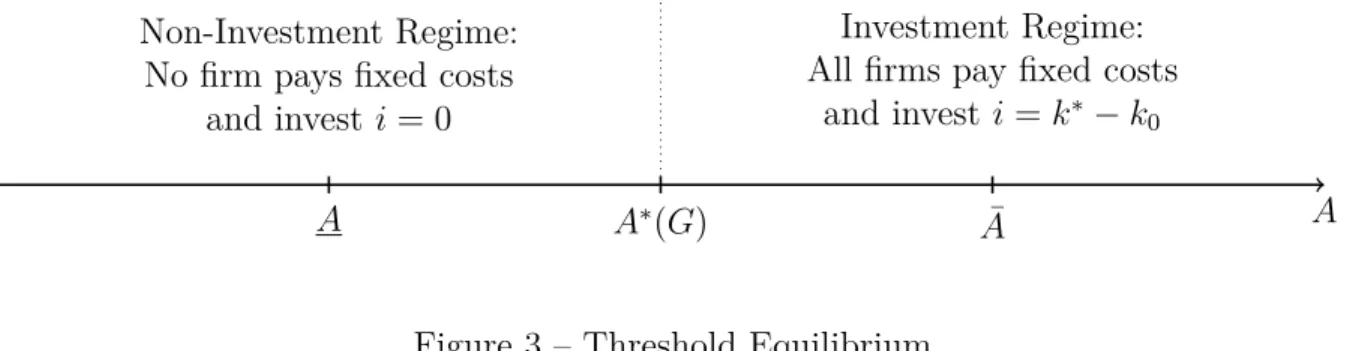
G), as the technology level which firms have the same expected profits of investing or not, taking in account expectations about other firms’ decisions. Moreover, the threshold determines two regimes: an investing regime that all firms are investing ifA≥A∗

(G), i.e,h= 1; and a non-investing regime ifA < A∗

(G), which h= 0.

(21)

A

A A∗

(G) _A¯

Non-Investment Regime: No ﬁrm pays ﬁxed costs

and invest i= 0

Investment Regime: All ﬁrms pay ﬁxed costs

and investi=k∗

−k₀

Figure 3 – Threshold Equilibrium

in Benhabib and Farmer (1999) and others, but they are pinned down by fundamentals in a unique threshold equilibrium. The advantage of our unique equilibrium is that it deﬁnes precisely when each regime happens.

An interesting feature of this equilibrium is that it can accommodate the evidence that investment bursts accounts for a large share of investment activity, as Cooper and Haltiwanger (2006) emphasize. Suppose, for instance, that the productivity level is lower but very close to the threshold. A small change in the productivity can lead to a burst in the investment rate. This would be wrongly interpreted as an increase in “animal spirits” of the economy that is not related to the economy fundamentals. However, it exactly the opposite. Hence, a model that incorporate this kind of general equilibrium effects on investment coordination may have a interesting discontinuous relationship with the economy fundamentals (in addition to the usual continuous relationship). Therefore, one need not to rely in very high fixed costs to accommodate the micro-data finding. 3

The economy has efficient aggregate investment in three cases. First, when A > A¯, all firms are investing because the productivity level is so elevated that firms find optimal to invest despite of other firms’ decisions. Second, when A ∈ (A∗

,A¯), all firms are investing but it is different from previous case. In this case, the technology level is not high enough to induce all firms to invest independently of others, but it is sufficiently high to induce firms to invest when they take into account the demand externalities from aggregate investment decisions. In other words, this is efficient as the productivity is sufficiently high to induce coordination between firms. Finally, the third case is when A < A which all households are not investing. It is also efficient as productivity is so low that for an individual firm it is optimal not to invest even though everyone is investing and then, in equilibrium no one invests.

Cooper and John (1988) emphasize the role of coordination failures in Keynesian models:

3

(22)

Figure 4 – Eﬀects of a increase in Government Expenditure in Threshold

“the economy can get stuck at an ineﬃcient equilibrium with a low level of “economic ac-tivity”, even though a better equilibrium exists”. Instead, we have this property in a unique equilibrium model. More precisely, when A∈(A, A∗

) the aggregate investment is ineﬃcient due to lack of coordination of investments. The economy get stuck in the non-investment regime with a low level of economy activity, even though we have a better possible outcome. In order to understand this point, for a given productivity level in the rangeA∈(A, A∗_),

sup-pose that there exist a mechanism for all ﬁrms to coordinate their investment decision so that

h= 1. Recall that, for a given G, A is deﬁned as the technology level that D(A,1, G) = 0.

Since D(A, h, G) is increasing in A, we have that D(A,1, G) > 0 for any A ∈ (A, A∗_{). In}

words, if all ﬁrms are investing, it is optimal to the individual ﬁrm decide to also invest. 4

Since the productivity threshold determines the equilibrium outcomes it is important to understand why it is a decreasing function of G. The ﬁgure 4 show the eﬀect of an increase in government expenditure in the productivity threshold. The increase from G to G′

> G

implies in a upward shift in the function D(A∗

(G), G) which leads to an lower threshold,

A∗₍

G′_).

However, it is possible to separate the effect of government spending on two channels. An increase in government expenditure induces the final good firm to demand more intermediate goods, which in turn, increases incentives to invest. This is a direct and partial equilibrium effect, which is the usual demand channel. We represent this as the shift to the of the initial curve D(A, G) to the dotted curve. The second is a general equilibrium channel that arises

4

(23)

from the fact that there is strategic uncertainty. Firms do not know exactly if other firms are investing or not. However, they expect that other firms also face higher demand. If they invest, aggregate demand increases and thus, more individual demand for each firm. Moreover, each of them expect that other firms expect that their individual demand will increase. This expectational process continues ad infinitum. The game theory literature call it higher-order beliefs. Because of this higher-order expectational channel, the curve shifts upward again, now from the dotted curve to the D(A, G′_{) curve. Therefore, there are more}

incentives to invest since firms require a lower level of productivity to be indifferent between investing or not. We call this channel as confidence channel since it captures expectations from firms on the other firms’ expectations about economy fundamentals. The productivity threshold is a sufficient statistic for this higher-order expectational (“confidence”) channel.

Our theoretical results are special related to the empirical evidence of Bachmann and Sims (2012). They use a non-linear VAR using three variables: output, government expen-diture and a measure of conﬁdence.5 _{Their main ﬁnding is that government expenditure has}

greater impacts in output during recessions than in expansions. In recessions, an increase in government expenditure leads to an increase in confidence at first 3 quarters and it starts to decrease slowly, but keeps always higher than the initial level of confidence. Moreover, output increases constantly with the peak of response after 20 quarters. In expansions, the effect on output is very short for only 5 quarters. When the confidence channel is shut off in their VAR, the impulse responses of recessions become very similar to their counterpart in expansions.

In the following we map this evidence with our results. Our model is static, but can be also understood as dynamic model with full depreciation of capital. In addition, we can think the productivity as a stochastic process instead of a constant. Since the only source of fluctuations in this model are the productivity shocks, we can interpret recessions (expansions) as low (high) values of A. Therefore, the confidence channel is more important precisely when there are more chances of a coordination failure. In figure 4, the second shift would be higher than the first one.

It is important to emphasize that Bachmann and Sims (2012) do not interpret their results as corresponding to the idea of a sentiment-induced surge as eﬀects in output are slowing building. Instead, they interpret it as increases in productivity induced by government expen-ditures in infrastructure and education. Our model instead imply a sharp change in output if the regime changes. However, there are several reasons why investment surges may be slow. The usual reasons are time to build or convex adjustment costs for investment. Maintaining heterogeneous information instead of taking the limiting case, or consider the case of

hetero-5

(24)

geneous fixed costs, both would lead to less abrupt shifts in aggregate investment as firms would have different cut-off strategies. However, we did not pursue these extensions.

The existence of this new general equilibrium conﬁdence channel opens a question whether government policies can help ﬁrms to coordinate their investments. The Proposition 1 has an answer. It shows that thresholdA∗₍

G) is a decreasing function ofG. Therefore, ﬁscal policy diminish the region where the aggregate investment is ineﬃcient and may induce individuals to increase investment. Suppose, for instance, that economy is in non-investing regime, that is, A < A∗₍

G). An increasing in the provision of public goods, increase the incentives for investing as the threshold decreases. This shift the region of inefficient investment to lower levels of productivity, alleviating the coordination problem. Moreover, if the productivity is sufficiently close to the threshold, it is possible that the government expenditure can shift the economy for the efficient regime that all firms are investing.

2.1 Market Clearing

The market clearing of goods market is given by:

Y =C+I +G=

  

 

YI(A, G) if A ≥A∗(G)

YN(A, G) if A < A∗(G)

(2.9)

where YI(A, G) ≡ Y(A,1, G) =

ωyI(A, Y(A,1, G))

θ₋₁

θ + (1−ω)G θ₋₁

θ

θ₋θ₁

is the aggregate output in the investing regime andYN(A, G)≡Y(A,0, G) =

(1−ω)yN(A)

θ₋₁

θ + (1−ω)G θ₋₁

θ

θ₋θ₁

for the non-investing regime. It is easy to see that YI(A, G) > YN(A, G). Notice that the

aggregate investment is given by:

I =

ˆ 1

0

C(ii)di=

  

 

k∗₍

A, YI(A, G))−k0+ψ if A ≥A∗(G)

0 if A < A∗₍

G) (2.10)

(25)

25

3 Optimal Fiscal Policy

It is clear from last section discussion that government decision can affect the investment decisions of the private sector. Until now, we found the equilibrium outcomes for a given government expenditure decided in first stage. Now, we will turn to the question on how would be the optimal decision of a social planner taking in account that fiscal policy can affect the threshold. Recall that, as we have coordination failures in the regionA∈(A, A∗_),

the social planner can improve welfare. However,A is also unobservable for the government it needs to maximize the representative expected household utility function based on an prior

g(A) over A, which is given by

E(U) =

ˆ ∞

−∞

u(C)g(A)dA (3.1)

subject to resource constraints. Inserting it in the welfare function, the government problem is now given by:

max

G

ˆ A∗(G)

−∞

u[YN(A, G)−G]g(A)dA

+

ˆ ∞

A∗₍_G₎

u[YI(A, G)−G−[k

∗

(A, YI(A, G))−k0+ψ]]g(A)dA (3.2)

The ﬁrst order condition of this problem is:

ˆ A∗(G)

−∞

u′

(CN(A, G))

"

∂YN(A, G)

∂G −1

#

g(A)dA

+

ˆ ∞

A∗₍_G₎

u′

(CI(A, G))

"

∂YI(A, G)

∂G −1−

∂k∗

∂Y

∂YI(A, G)

∂G

#

g(A)dA (3.3) −∂A

∗

(G)

∂G (u[CI(A

∗

(G), G)]−u[CN(A

∗

(G), G)])g(A∗

(G)) = 0

whereCN(A, G) =YN(A, G)−Gand CI =YI(A, G)−G−[k∗(A, YI(A, G))−k0 +ψ] are the

(26)

Chapter 3. Optimal Fiscal Policy 26

ﬁscal policy is equalizing the marginal beneﬁt resulting of higher expenditure of public goods to the marginal cost of consumption crowding-out.

Let us turn now to the third term, which relates to the conﬁdence channel that arises as there are coordination problem in investments. Proposition 1 shows that ∂A∗₍_G₎

∂G < 0

and thus, the third term represents the welfare increase of changing to the investment regime when the economy has exactly the productivity equal to the threshold, i.e.,u[CI(A∗(G), G)]−

u[CN(A∗(G), G)]. Notice that this eﬀect is proportional to the prior probability of economy

is close to the threshold, i.e., g(A∗₍

G)). Therefore, the more likely a coordination problem, the more this channel is important in government expenditure choice.

In the following, denote G∗

c the optimal government expenditure when there are

coordi-nation failures and G∗

denote the optimal government expenditure when ∂A∗₍_G₎

∂G = 0. When

we impose that ∂A∗₍_G₎

∂G = 0 we are shutting off the confidence channel of fiscal policy. The

following proposition show the diﬀerence of the optimal government in both cases.

Proposition 2. Denote G∗

c as the government expenditure level which solves equation 3.3,

and G∗

which solves the same equation when ∂A_∂G∗(G) = 0. Therefore, G∗

c ≥ G

∗

, for any distributiong with support on the real line.

The proof is in the appendix. This result shows that under the threat of coordina-tion failures, the optimal fiscal policy is to choose to produce beyond the point where the marginal benefit resulting from the consumption of public goods equals the marginal cost of those goods. It is so because government spending has an indirect effect on firms’ expecta-tions, enhancing coordination. To show this result, we need to prove that CI(A∗(G), G) >

CN(A∗(G), G). That is for a given G, if technology is so that ﬁrms are indiﬀerent between

investing or not, i.e., A = A∗₍

G), if ﬁrms happens to go to the investing regime, the con-sumption is higher than otherwise. This guarantees that the third term in the 3.3 is positive, i.e., government expenditure increase the expected household utility as it diminishes the threshold.

Another way to see this is shown in Figure 5. Without the threat of coordination failures or equivalently, shutting off the confidence channel of fiscal policy, the optimal government expenditure isG∗

(27)

Chapter 3. Optimal Fiscal Policy 27

Figure 5 – Optimal government expenditure under the threat of coordination failures

the ﬂat line.1 _{Therefore, government must use ﬁscal policy to create more demand, increasing}

“conﬁdence” of individual ﬁrms in the economy aggregate investment that may lead to change in the investment regime. This increases expected representative welfare.

So our model says that government expenditure should always to increase more? The answer is no. There is the usual trade-oﬀ between the increase in output and government expenditure with a larger share of output. Moreover, when our additional channel is taken into account, the optimal increase in expenditure is proportional to the likelihood which government assigns to a coordination problem, i.e., g(A∗₍

G)). Therefore, when the coordi-nation problem is unlike, for instance, it is attributed a high probability of a period of very high productivity the diﬀerence between the government expenditure taking into account our channel from the usual problem is negligible.

1

This additional expected loss is a function ofG_{, so it is not a flat line. However, since we know that it is}

(28)

28

Concluding Remarks

We proposed a static model with monopolistic competition and fixed costs, in which invest-ment decisions are subject to informational frictions about aggregate productivity level. This setup delivers a model where higher-order expectations are key. When government supply public goods that are imperfect substitutes of private goods, fiscal policy has two effects in aggregate demand: the direct effect that is usually emphasized and the confidence effect that affect investment incentives. This channel arises as firms face strategic uncertainty about other firms’ investment decisions that may lead to investment coordination failures. Tak-ing this channel into account, that is, under the threat of coordination failures, the optimal fiscal policy is to produce beyond the point where the marginal benefit resulting from the consumption of public goods equals the marginal cost of those goods. This additional benefit comes from the fact that fiscal policy can enhance investment coordination.

To our knowledge, this is the first paper to attempt to understand a confidence channel for fiscal policy in theoretical grounds. Moreover, despite the recent growing literature making use of imperfect common knowledge type of information friction is business cycles, this paper is first to use global games in lines of Morris and Shin (2003) in a macroeconomic model.

(29)

29

A Appendix - Proofs

A.1 Proof of Lemma 1.

For convenience, lets rewrite the important equations with all arguments explicit to derive the ﬁxed point:

Y(A, h, G) = ωhhyI(A, Y(A, h, G))

θ₋1

θ + (1−h)y

N(A)

θ₋1

θ

i

+ (1−ω)Gθ−θ1

θ θ₋1

(A.1)

yI(A, Y(A, h, G)) =

"

αω θ−1

θ

!#

αθ θ(1−α)+α

A θ θ₍₁₋α₎₊α_Y

α

θ₍₁₋α₎₊α (A.2)

yN(A) =Akα0. (A.3)

After derivations, we drop the arguments in functions for notational convenience. In equation A.1, when Y = 0, we have that LHS = 0 and RHS ≥ 0, for G ≥ 0. Taking the derivative ofRHS with respect to Y:

∂RHS

∂Y =ω(Y)

1

θ

"

hy θ₋₁

θ −1

I ∂yI ∂Y # =ω _y I Y

θ₋₁ θ "

h∂yI ∂Y

Y yI

#

≥0 (A.4)

which is clearly strictly positive unless h = 0. The case where h = 0 is trivial since RHS

(right hand side) do not depend onY. In the case that h ∈(0,1], since yI is concave in Y,

it is easy to see that yI

Y is decreasing in Y. As ∂yI

∂Y Y yI =

α

θ(1−α)+α is constant and θ > 1, this

implies that RHS is concave on Y. Moreover, limY→∞ ∂RHS_∂Y = 0. Figure 6 shows RHS as

function of Y for both cases. As LHS (left hand side) is the 45 degrees line, both curves intersect only once for both cases. In the case whereh∈(0,1], in the crossing point, we have that ∂RHS

∂Y < 1. Therefore, we have a unique ﬁxed point solution for Y(A, h, G) for a given

(A, h, G).

Using the implicit function theorem, we have that the derivatives of each argument are:

∂Y(A, h, G)

∂A =

ω(Y)1θ

h

hyI

θ₋₁ θ −1∂yI

∂A + (1−h)yN

θ₋₁ θ −1∂yN

∂A

i

1− ∂RHS ∂Y

(A.5)

= ω(Y)

−θ−1

θ

h

hyI

θ₋1

θ ∂yI

∂A A

yI + (1−h)yN θ₋1

θ ∂yN

∂A A yN

i

(30)

Appendix A. Appendix - Proofs 30

Figure 6 – Fixed Point solution

∂Y(A, h, G)

∂G =

(1−ω)Y G

1θ

1− ∂RHS ∂Y

>0 (A.7)

∂Y(A, h, G)

∂h =ω(Y)

1

θ

y θ θ₋₁

I −y

θ θ₋₁

N

1− ∂RHS ∂Y

(A.8) Which ∂RHS

∂Y is deﬁned as in A.4. Notice that for A and G the signal is clearly positive as

yI and yN are increasing functions ofA and, in equilibrium, ∂RHS_∂Y <1. Now lets turn to the

derivative with respect toh. Sincei≥0 because of the irreversibility of capital, thenk∗

≥k0

which implies thatyI ≥yN. Then ∂Y(A,h,G_∂h ) >0.

A.2 Proof of Lemma 2.

For convenience, lets rewrite the equations 2.3 and 2.4

ˆ

πI(A, h, G) =ω(yI(A, Y(A, h, G)))

θ₋₁

θ _Y(_{A, h, G})1θ −[k∗(A, Y(A, h, G))−k

0]−ψ (A.9)

ˆ

πN(A, h, G) = ωyN(A)

θ₋₁

θ Y(A, h, G)

1

(31)

Suppose a pair (A, h) and the optimal choice k∗

. Lets denote ∆A a small change in A. The change in proﬁts for the non-investing ﬁrm is

∆ˆπN =ω

"

θ−1

θ ω

y θ₋₁

θ −1

N ∆yN

Y 1θ +1 θy

θ₋₁ θ

N Y

1

θ−1∆Y

#

∆A (A.11)

Now suppose an arbitrary choice for the investing firm: doing exactly the same decision of the non-investing firm, i.e., keepk∗ _{constant. Since the fixed cost is already payed, it does}

not matter for the change in profits. Since the investing firm can adjust capital freely, this strategy is in their frontier of possibilities of production. This implies that it have at least the same profits of this strategy:

∆ˆπI ≥ω

"

θ−1

θ

y θ₋1

θ −1

I ∆yI

Y 1θ + 1 θy

θ₋1

θ

I Y

1

θ−1∆Y

#

∆A (A.12)

Lemma 1 guarantees that ∆Y > 0. Then, ∆D = ∆ˆπI−∆ˆπN with this small change in

A is

∆D≥ω

"

θ−1

θ

y θ₋1

θ −1

I ∆yI−y

θ₋1

θ −1

N ∆yN

Y 1θ + 1 θ

y θ₋1

θ

I −y

θ₋1

θ

N

Y 1θ−1∆Y

#

∆A (A.13) Taking the limit ∆A→0 we have that

∂D

∂A ≥ω

"

θ−1

θ

"

y θ₋1

θ −1

I

∂yI

∂A −y

θ₋1

θ −1

N

∂yN

∂A

#

Y 1θ +1 θ

y θ₋1

θ

I −y

θ₋1

θ

N

Y 1θ−1∂Y ∂A

#

(A.14) multiplying forA in both sides

∂D

∂AA ≥ ω

"

θ−1

θ

"

y θ₋₁

θ I ∂yI ∂A A yI −y θ₋₁

θ N ∂yN ∂A A yN #

Y 1θ +1 θ

y θ₋₁

θ

I −y

θ₋₁ θ

N

Y 1θ∂Y ∂A

A Y

#

(A.15)

since ∂yI

∂A A yI =

(θ−₁₎₍₁−α)+θ θ(1−α)+α >1,

∂yN

∂A A

yN = 1, then: ∂D

∂AA > ω

"

θ−1

θ

y θ₋₁

θ

I −y

θ₋₁ θ

N

Y 1θ +1 θ

y θ₋₁

θ

I −y

θ₋₁ θ

N

Y 1θ∂Y ∂A

A Y

#

(A.16) Lemma 1 guarantees that ∂Y

∂A A

Y >0. As i ≥ 0 because of the irreversibility of capital, then

k∗

≥k₀ which implies that yI ≥yN. Hence, ∂D_∂A >0.

Let us turn now for the derivative with respect to h. Lets denote ∆h a small change in

h. Using the same argument as before we can ﬁnd

∆ˆπN =ω

1

θy θ₋₁

θ

N Y

1

θ−1∆Y

(32)

∆ˆπI ≥ω

1

θy θ₋₁

θ

I Y

1

θ−1∆Y

∆h (A.18)

Taking the diﬀerence and using the limit ∆h→0 we have that

∂D

∂hh≥ω

"

1

θ

y θ₋₁

θ

I −y

θ₋₁ θ

N

Yθ1∂Y ∂h

h Y

#

(A.19) Lemma 1 guarantees that ∂Y

∂h h

Y > 0. As i ≥ 0 because of the irreversibility of capital,

then k∗

≥k0 which implies that yI ≥yN. SinceyI is increasing in Y, we have that ∂D_∂h >0

Finally, lets turn to the derivative with respect toG. Since hand Gaffect profits only by their indirect effect through Y(A, h, G), the proof forG exactly the same as for h, changing ∆h(∂h) to ∆G(∂G).

A.3 Proof of Proposition 1.

Proof. The proof is a direct application of the Proposition 2.2 in Morris and Shin (2003). It is only necessary to check if the necessary and suﬃcient conditions are met. There are ﬁve assumptions to hold to guarantee the unique threshold equilibrium:

1. Action Monotonicity: D(A, h, G) is non decreasing in h. 2. State Monotonicity: D(A, h, G) is non decreasing in A.

3. Uniform Limit Dominance: For a given G, there exists A(G)∈ ℜ, ¯A(G) ∈ ℜ and ε ∈ ℜ++, such that (i): D(A, h, G)<−εfor allh∈[0,1] andA < A(G); (ii)D(A, h, G)> ε

for all h∈[0,1] and A >A¯(G). 4. Continuity: ´1

0 f(h)D(A, h, G)dh is continuous with respect to A and density f.

5. Finite Expectations of Signals: ´∞

−∞zf(z)dz is well deﬁned.

Conditions 1 and 2 are satisﬁed by Lemma 2. It is easy to see that D(0, h, G) < 0 and

limA→∞D(A, h, G) > 0 so that Condition 4 is satisﬁed. Condition 5 holds as D(A, h, G)

is continuous in all arguments and 6 by hypothesis (E(ε) = 0). Since condition 1 and 4 holds, we have the Strict Laplacian State Monotonicity condition. That is, for a given G, there exists a unique A∗₍

G) solving ´1

0 D(A ∗₍

G), h, G)dh = 0. Finally, since D(A, h, G) is increasing in G, then ´1

0 D(A ∗₍

G), h, G)dh is also increasing in G. Therefore, A∗₍

(33)

A.4 Proof of Proposition 2.

Proof. For convenience lets rewrite the ﬁrst order condition:

ˆ A∗(G)

−∞

u′

(CN(A, G))

"

∂YN(A, G)

∂G −1

#

g(A)dA

+

ˆ ∞

A∗₍_G₎

u′

(CI(A, G))

"

∂YI(A, G)

∂G −1−

∂k∗

∂Y

∂YI(A, G)

∂G

#

g(A)dA (A.20) −∂A

∗₍

G)

∂G (u[CI(A

∗

(G), G)]−u[CN(A

∗

(G), G)])g(A∗

(G)) = 0

Recall thatG∗ _{is such that the ﬁrst and the second term of the optimal solution for}

govern-ment is equal to zero. The Proof of Lemma 1shown that the expenditure multiplier is given by:

∂Y(A, h, G)

∂G =

(1−ω)Y G

1θ

1−∂RHS ∂Y

(A.21) is decreasing inGfor any (A, h). Hence, the net marginal welfare of government expenditures equals zero with negative slope, as illustrated in Figure 5. Therefore, if the third term is positive, then G∗

c > G

∗

as it is a upward shift in the condition which still has to be zero. From Proposition 1 we know that ∂A∗₍_G₎

∂G <0 and thus, the third term is positive, if and only

ifCI(A

∗

(G), G)> CN(A

∗

(G), G). This happens when the diﬀerence of outputs between both regimes is higher then the investment, as government expenditure is equal in both regimes, that is,YI(A∗(G), G)−YN(A∗(G), G)> k∗(A∗(G), YI(A∗(G), G))−k0+ψ.

By the deﬁnition of A∗₍

G) from Proposition 1, we know that:

ˆ 1

0

ω

(yI(A

∗

(G), Y(A∗

(G), h, G)))θ−θ1 −y

N(A

∗

(G))θ−1

θ

Y(A∗

(G), h, G)1θ−

dh

ˆ 1

0

[k∗

(A∗

(G), Y(A∗

(G), h, G))−k0]dh−ψ = 0 (A.22)

we can ﬁnd the inequality

0 = ˆ 1 0 ω

(yI(A

∗

(G), Y(A∗

(G), h, G)))θ−θ1 −_y

N(A

∗

(G))θ−1

θ

Y(A∗

(G), h, G)1θ

−[k∗

(A∗

(G), Y(A∗

(G), h, G))−k₀]−ψ

dh

< ˆ 1

0

{Y(A∗

(G), h, G)−[k∗

(A∗

(G), Y(A∗

(G), h, G))−k₀]−ψ}dh < YI(A

∗

(G), G)−YN(A

∗

(G), G)−[k∗

(A∗

(G), YI(A

∗

Investment coordination failures and the confidence channel of fiscal policy

INVESTMENT COORDINATION FAILURES AND THE

CONFIDENCE CHANNEL OF FISCAL POLICY

INVESTMENT COORDINATION FAILURES AND THE

CONFIDENCE CHANNEL OF FISCAL POLICY

INVESTMENT COORDINATION FAILURES AND THE

CONFIDENCE CHANNEL OF FISCAL POLICY

RESUMO

ABSTRACT

Contents

Introduction

1 Model

1.1

Firms

1.2

Information and Timing

1.3

Households and Government

2 Equilibrium

2.1

Market Clearing

3 Optimal Fiscal Policy

Concluding Remarks

A Appendix - Proofs

A.1

Proof of Lemma 1.

A.2

Proof of Lemma 2.

A.3

Proof of Proposition 1.

A.4

Proof of Proposition 2.