COnstructing Proxy-Record Age models (COPRA)

(1)

CPD

8, 2369–2408, 2012

COnstructing Proxy-Record Age

models (COPRA)

S. F. M. Breitenbach et al.

Title Page

Abstract Introduction

Conclusions References

Tables Figures

◭ ◮

Back Close

Full Screen / Esc

Printer-friendly Version Interactive Discussion

Discussion

P

a

per

|

Dis

cussion

P

a

per

|

Discussion

P

a

per

|

Discussio

n

P

a

per

|

Clim. Past Discuss., 8, 2369–2408, 2012 www.clim-past-discuss.net/8/2369/2012/ doi:10.5194/cpd-8-2369-2012

Climate of the Past Discussions

This discussion paper is/has been under review for the journal Climate of the Past (CP). Please refer to the corresponding final paper in CP if available.

COnstructing Proxy-Record Age models

(COPRA)

S. F. M. Breitenbach1, K. Rehfeld2,3, B. Goswami2,4, J. U. L. Baldini5,

H. E. Ridley5, D. Kennett6, K. Prufer7, V. V. Aquino7, Y. Asmerom8, V. J. Polyak8,

H. Cheng9, J. Kurths2, and N. Marwan2

1

Geological Institute, Department of Earth Sciences, ETH Zurich, 8092 Zurich, Switzerland

2

Potsdam Institute for Climate Impact Research (PIK), 14412 Potsdam, Germany

3

Department of Physics, Humboldt Universit ¨at zu Berlin, Newtonstr. 15, 12489 Berlin, Germany

4

Department of Physics, University of Potsdam, Karl-Liebknecht Str. 24–25, 14476 Potsdam, Germany

5

Department of Earth Sciences, Durham University, Durham, DH1 3LE, UK

6

Department of Anthropology, The Pennsylvania State University, University Park, PA 16827, USA

7

Department of Anthropology, University of New Mexico, Albuquerque, USA

8

Department of Earth and Planetary Sciences, University of New Mexico, Albuquerque, New Mexico, USA

9

(2)

CPD

8, 2369–2408, 2012

models (COPRA)

Title Page

Tables Figures

◭ ◮

Back Close

Full Screen / Esc

Discussion

P

a

per

|

Dis

cussion

P

a

per

|

Discussion

P

a

per

|

Discussio

n

P

a

per

|

Received: 5 June 2012 – Accepted: 6 June 2012 – Published: 19 June 2012

Correspondence to: S. F. M. Breitenbach (breitenbach@erdw.ethz.ch)

(3)

CPD

8, 2369–2408, 2012

models (COPRA)

Title Page

Tables Figures

◭ ◮

Back Close

Full Screen / Esc

Discussion

P

a

per

|

Dis

cussion

P

a

per

|

Discussion

P

a

per

|

Discussio

n

P

a

per

|

Abstract

Reliable age models are fundamental for any palaeoclimate reconstruction. Interpo-lation procedures between age control points are often inadequately reported, and available modeling algorithms do not allow incorporation of layer counted intervals to improve the confidence limits of the age model in question. We present a modeling

ap-5

proach that allows automatic detection and interactive handling of outliers and hiatuses. We use Monte Carlo simulation to assign an absolute time scale to climate proxies by conferring the dating uncertainties to uncertainties in the proxy values. The algorithm allows us to integrate incremental relative dating information to improve the final age model. The software package COPRA1.0 facilitates easy interactive usage.

10

1 Introduction

Palaeoclimate reconstructions are a way to relate recent variability in climatic pattern to past changes and to discuss the significance of such changes. They are based on proxy records, retrieved from a large variety of natural archives such as trees, glaciers, speleothems, or sediments. Such archives store information about climate parameters

15

in stratigraphic, and, hence, chronological order.

The proxy-record in question is generally given against depth and must be related to a time scale before any attempt of interpretation can be made. This is done by dating individual points within the sediment column using layer counting, radiometric dating

(14C-, or U-series), or marker horizons (e.g. tephrochronology). The (growth-)

depth-20

age relationship can be determined for each proxy data point (the actualage

model-ing). Limitations on sample material, analytical costs, and time considerations allow for

dating of only a few points within a proxy record, and various methods are employed for the age modeling process. Naturally, the quality of any age model depends on the number of dates and the associated uncertainties (Telford et al., 2005).

(4)

CPD

8, 2369–2408, 2012

models (COPRA)

Title Page

Tables Figures

◭ ◮

Back Close

Full Screen / Esc

Discussion

P

a

per

|

Dis

cussion

P

a

per

|

Discussion

P

a

per

|

Discussio

n

P

a

per

|

Inevitably, each dating method comes with inherent uncertainties, and herein lies one basic caveat for any climate reconstruction: the time frame is not as absolute (i.e. pin-pointed in time) as one wishes and the uncertainties must be accounted for when interpreting these proxies. Dating uncertainties are often only discussed for dis-crete dated points, rather than the entire age model. Blaauw et al. (2007) and Blaauw

5

(2010) present possible ways of resolving this issue. Scholz and Hoffmann (2011) point

out that the interpolation procedures and techniques used are often not described in

adequate detail and lack of consistency and objectivity can cause difficulties when

dif-ferent records are to be compared or reanalyzed, or wherever leads and lags between

different reconstructions are studied. The problem is becoming more acute because

10

the spatio-temporal coverage of proxy records now allows for direct network analysis (Rehfeld et al., 2011) and more quantitative reconstructions (Hu et al., 2008; Medina-Elizalde and Rohling, 2012). In order to obtain meaningful results from such studies, we must be able to consider the uncertainties of the records being compared.

Establishing a methodology for comparing different proxy records is challenging

be-15

cause of the apparent uncertainties in the ages at which the proxy values are known. Such a method would require something equivalent to the “inertial frame of reference” in physics – a reference system that possesses certain universally valid properties without exception. In the particular case of proxy record construction, such an invariant

“referential” quantity isphysical time. Physical time is the same for any proxy source,

20

and the di_fferences arise only in the deposition, growth, measurement and finally, the

estimation of the proxy in question. In this study we establish a method for constructing such an “absolute” time scale for any and all proxy records.

The primary goal of age modeling is to construct meaningful time series that relate uncertainties in climate proxies with age–depth relationships and associated errors.

25

(5)

CPD

8, 2369–2408, 2012

models (COPRA)

Title Page

Tables Figures

◭ ◮

Back Close

Full Screen / Esc

Discussion

P

a

per

|

Dis

cussion

P

a

per

|

Discussion

P

a

per

|

Discussio

n

P

a

per

|

hidden. All available approaches aim to construct one “ideal” age model to which the proxy information is related.

Several techniques have been developed to construct consistent age models and

un-certainty estimates (Blaauw et al., 2007; Bronk Ramsey, 2008; Scholz and Hoffmann,

2011). The most recent one is StalAge (Scholz and Hoffmann, 2011), a routine that

5

helps to interpolate between dated points and uncertainty estimation for intervening and undated points in between. StalAge is especially suitable for speleothem U-series age modeling (though in principle it can be used also for other archives, such as lake sediments or ice cores) and allows for detection and handling of outlier and hiatuses. However, age model constructions can be further improved with the incorporation of

ad-10

ditional information into the numerical procedure, such as counted intervals between at least two “absolute”-dated points. Here, we introduce a novel approach to age model-ing that not only overcomes some of the caveats mentioned above but also attempts to integrate the pragmatic and theoretical aspects of reconstructing a proxy record from the measurement data in a holistic framework. Moreover, this approach allows the

as-15

signment of the proxy values to an absolute (or true) time scale by translating the dating uncertainties to uncertainties in the proxy values.

An absolute time scale is the true chronological date at which time the sample was deposited. Usually, the most likely age is somehow assigned to a measured proxy value. But now we pose the converse question: which proxy value is most likely for

20

a given year? Instead of considering ages with uncertainties, we now have the uncer-tainty in the proxy value. Considering the absolute time would have the benefit that we

can compare all the different proxy records directly, because their time axes are

iden-tical, fixed, and without any error. These time axes are not necessarily equidistant, but could also have non-equidistant time points.

25

(6)

CPD

8, 2369–2408, 2012

models (COPRA)

Title Page

Tables Figures

◭ ◮

Back Close

Full Screen / Esc

Discussion

P

a

per

|

Dis

cussion

P

a

per

|

Discussion

P

a

per

|

Discussio

n

P

a

per

|

outliers and hiatuses, and narrow the age uncertainty by supplying additional informa-tion, such as layer counting data. As an implementation of this algorithm, we present COPRA1.0, an interactive interface-based age modeling software that allows

– detection, classification, and treatment of age reversals;

– detection and treatment of hiatuses;

5

– interpolation between discrete dating points;

– optional inclusion of layer counting information (thereby potentially including

non-linear accumulation behavior between dating points);

– mapping of the proxy records to an absolute time scale and estimation of proxy

record uncertainties which inherently take into account the uncertainties of the

10

age model.

The interface allows the specialist to handle suspect data and/or include additional information in order to improve the final age model. The software logs and exports all relevant meta-data to ensure reproducibility. We hope that this software routine will help palaeoclimatologists to construct reliable and reproducible age models for their proxy

15

records.

2 Methods

2.1 General remarks

The determination of a reliable chronology, relating proxy changes to certain dates in the past, is a challenge in most paleoclimate archives. The depth (i.e. the distance from

20

(7)

CPD

8, 2369–2408, 2012

models (COPRA)

Title Page

Tables Figures

◭ ◮

Back Close

Full Screen / Esc

Discussion

P

a

per

|

Dis

cussion

P

a

per

|

Discussion

P

a

per

|

Discussio

n

P

a

per

|

obtained at only a few depths to the depths of the proxy measurements yields the age-versus-proxy relationship, and is the primary task of age modeling.

For age modeling, we need two datasets – one with dated points and another with proxy values – each with their respective depths from the stalagmite top. Additional information on marker layers (e.g. hiatuses), and other specific information might be

5

provided as well. In order to compile the optimal input for age modeling, the direct dating information, here the U-series dated samples and their geochemical behavior, and mineralogical and petrographic environment, should be evaluated by the special-ist. Information on sampling depth, possible contamination, hiatuses, or geochemical alterations might be available and can greatly help to identify outliers prior to any

mod-10

eling.

Dating a record is possible using different kinds of information (as outlined above),

and depends on the type of archive. Before we proceed to describe the algorithm, we have to distinguish between point estimates and incremental dating.

Point estimates, i.e. age estimates at the date points provide the only “absolute”

15

chronological information1. If the archive is actively accumulating then the top of the

sequence also provides an absolute date. While there are several forms of pointwise age-estimates, their treatment in age modeling is usually generic and we will focus on

U-series dates in particular. Radiometric dates (like U-series or14C) come with

mea-surement uncertainties, so although they might be “absolute”, they are not “exact”. In

20

the context of the COPRA algorithm, we assume that the uncertainty distribution of the U-series date (or any other pointwise age estimate) is Gaussian, and the standard devi-ation is given. Gaussianity presents a simplificdevi-ation, and is certainly not always correct (Blaauw, 2010). In the case of very high precision dates additional uncertainty might

1

(8)

CPD

8, 2369–2408, 2012

models (COPRA)

Title Page

Tables Figures

◭ ◮

Back Close

Full Screen / Esc

Discussion

P

a

per

|

Dis

cussion

P

a

per

|

Discussion

P

a

per

|

Discussio

n

P

a

per

|

result from the physical sampling procedure, if the analytical error in years is smaller

than the years integrated by sampling. At su_fficiently high growth rates, this “sampling

contribution” becomes negligible. Currently we do not propagate this “sampling uncer-tainty” in our modeling routine, but with future analytical improvements this additional uncertainty must be considered.

5

Incremental dating can be obtained if the archive growth is seasonally or annually structured. If this is the case, annual layers might be distinguished, e.g. from crystal-lographic, or geochemical changes (Treble et al., 2005; Mattey et al., 2010; Fairchild et al., 2006). Starting at a known date, the years can be counted backwards (from the top or the most recent section). This is a standard procedure in tree ring and ice

10

core chronology building, and sometimes, in speleothems or lake sediments (Marwan et al., 2003; Mattey et al., 2010; Preunkert et al., 2000; Svensson et al., 2008; von Rad et al., 1999). In this case, highly resolved information about the age–depth relationship is available and should, if possible, be included in the age modeling procedure in order to improve the uncertainty estimates of the model. The COPRA algorithm can make

15

use of incremental dating and its implementation in COPRA1.0, such layer counting information can be provided for any section of the core.

In summary, the fundamental assumptions are:

– Age measurements (both pointwise and incremental) are assumed to be the

ex-pectation value of a normally distributed random variable with the standard

devi-20

ation equalling the measurement error.

– An exhaustive computer-aided search of all stratigraphically possible (i.e.

mono-tonic) relationships within the normally distributed age observations will help quantify the most realistic age model within the limits of measurement uncertainty.

– In cases where the stratigraphic condition is violated at the level of the age

ob-25

(9)

CPD

8, 2369–2408, 2012

models (COPRA)

Title Page

Tables Figures

◭ ◮

Back Close

Full Screen / Esc

Discussion

P

a

per

|

Dis

cussion

P

a

per

|

Discussion

P

a

per

|

Discussio

n

P

a

per

|

proper treatment (age reversals), (2) a physical event in the archives accumulation history caused the observations to deviate from typical stratigraphic monotonicity and thus have to be treated accordingly (e.g. in case of hiatuses).

– Incremental dating information amounts to additional knowledge about the age–

depth relation and hence, when incorporated into the age model, should reduce

5

the overall uncertainty.

The COPRA algorithm should enable reliable and reproducible age modeling for proxy time series. Therefore, any COPRA implementation has to record all necessary information required to reproduce the age modeling, including the input dating informa-tion (depth, error, age, error), input proxy values, informainforma-tion on layer counts (if given),

10

and all information on the modeling, like number of Monte Carlo (MC) realisations, in-terpolation used (cubic, spline, linear), excluded dates, enlarged error bars, confidence interval details, etc.

2.2 Monte Carlo modeling: the core of COPRA

Fundamental to the COPRA algorithm is the creation of the age model that accounts

15

for the age uncertainties. In general, the age model is derived by an interpolation of the few dates in the dating table towards the higher-resolution depth scale of the proxy measurements. Each dated point is provided with an error value corresponding to

a standard deviationσof a normal distribution. This means that for each location dated

the most likely age is represented by the peak in the distribution, but also other ages

20

(younger and older) are possible, with lower probability. The probability of these slightly

differing ages is specified by the normal distribution and its standard deviation σ. For

example, aσvalue of 5 yr would mean that with 5 % probability the given age could be

10 yr older or 10 yr younger than actually specified (the 95 % confidence interval can

be estimated as 2σ).

25

(10)

CPD

8, 2369–2408, 2012

models (COPRA)

Title Page

Tables Figures

◭ ◮

Back Close

Full Screen / Esc

Discussion

P

a

per

|

Dis

cussion

P

a

per

|

Discussion

P

a

per

|

Discussio

n

P

a

per

|

T_i and standard deviationsσ_iT of the age estimatesT_i. Here, for matters of simplicity, we

shall require thatD_i₊₁> D_i, i.e. the depths at which ages are measured should always

be reported in increasing order. Now, in order to incorporate the dating uncertainties

σ_iT into the age model, COPRA adds small numbers drawn from a normal distribution

with standard deviationσ_iT to the agesTi and interpolates the ages to the proxy record.

5

Repeating this many times, we get many slightly differing age models populating the

confidence intervals of the dating points (defined within COPRA as different realizations

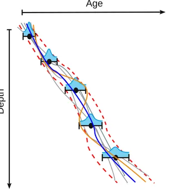
of the final age model, cf. Fig. 1).

These age model realizations demonstrate the uncertainties of the ages given by the

dating errors and allow the construction of an age distribution for the given depthD_i,

10

formallypi(Ti|Di). The median of these realizations for each depth valueDi of the proxy

record reveals the most likely ageTi for this sample positioni; and the quantiles of the

corresponding age distribution for each depth value can be used to infer the confidence interval for the corresponding ages (Fig. 1). However, the shape of these confidence intervals depends on the chosen interpolation (linear, cubic, spline). This procedure is

15

known as Monte Carlo (MC) simulation, and the default number of MC realizations in COPRA is 100.

A further precondition for the interpolation is monotonicity – arising from the strati-graphic reasoning that in almost all palaeoclimatic archives “deeper is older”. Therefore non-tractable age reversals within the dating table have to be excluded beforehand

(dis-20

cussed in further detail in Sect. 2.3). Still, due to the addition of small random numbers to the ages, in some realizations the monotonicity might not be preserved if the age errors of the dated samples are largely overlapping. Such realizations will be dropped and a new Monte Carlo iteration is added (brown curve in Fig. 1). In some extreme cases this can lead to a very large number of realizations to be calculated until the

pre-25

(11)

CPD

8, 2369–2408, 2012

models (COPRA)

Title Page

Tables Figures

◭ ◮

Back Close

Full Screen / Esc

Discussion

P

a

per

|

Dis

cussion

P

a

per

|

Discussion

P

a

per

|

Discussio

n

P

a

per

|

Based on the age model realizations, we derive for each proxy value a distribution of

corresponding agespi(Ti|Di) (now assigned to the depth scale of the data). However,

the ensemble of age model realizations also allows us to construct an absolute (or true) time scale, to which we assign the likely proxy values. This is done by calculating

the distribution of the positions in the record at a given agepj(Dj|Tj) (using

interpo-5

lation). For each ageT_j we can now calculate the distribution of proxy values. By this

procedure we translate the dating uncertainties into proxy value uncertainties. As al-ready mentioned, absolute time scales have the advantage that they allow comparison

of different records, even if they are differently dated.

2.3 Outliers and age reversals

10

Outliers and age reversals are a main cause for problems in the construction of age models. Outliers can significantly change the age–depth relationship and age reversals violate the fundamental assumption of monotonicity, i.e. positive growth of the deposit. COPRA detects both, outliers and age reversals, and helps the decision-making pro-cess for further handling of these problematic dating points. Outliers should usually be

15

excluded, whereas reversals could be excluded or handled by their error distribution. The COPRA implementation marks outliers and age reversals and allows the user to interactively apply an appropriate handling procedure, i.e. exclusion, handling within the error margins, or even increasing the error margins if feasible.

2.3.1 Outliers

20

An outlier is a dating point that is obviously not consistent with the growth history of an

archive. Outliers can occur for di_fferent reasons, e.g. geochemical alterations,

contam-inated samples, or measurement errors. Such ages appear outside the general trend of the rest of the age–depth relationship. Removing an outlier usually strongly alters the general shape of the age–depth relationship. However, the “true” growth history of

25

(12)

CPD

8, 2369–2408, 2012

models (COPRA)

Title Page

Tables Figures

◭ ◮

Back Close

Full Screen / Esc

Discussion

P

a

per

|

Dis

cussion

P

a

per

|

Discussion

P

a

per

|

Discussio

n

P

a

per

|

an outlier does not necessarily lead to an age reversal. Therefore, besides the obvious appearance of an outlier in an age–depth plot, it is important to cross-check this finding with the proxy material.

In many (speleothem) cases, samples can be identified as “outliers” for example due to high detrital thorium concentrations or because mineralogical analysis hints to

al-5

tered segments in the stalagmite (e.g. aragonite to calcite diagenesis). The geochem-ical data obtained during U-series analysis help evaluate the sample for unforeseen chemical changes (like leaching). Therefore it is the scientist who must evaluate the

geochemical data in its overall sedimentological/geological context. Samples affected

by such influences should be marked and treated with extra care. If independent

infor-10

mation proves outliers to have undergone alteration they might be excluded from further calculations prior to the age modeling procedure. Such evidence could be geochemical

data, X-ray diffraction (XRD) results pointing to diagenesis, or other information.

How-ever, if no other evidence proves the exceptional behavior of the sample, simple ex-clusion is generally not easily justified. Other sophisticated methods on outlier-analysis

15

and -handling have been described (e.g. Bronk Ramsey, 2009), but these are beyond the scope of COPRA1.0 and might be explored in subsequent studies.

2.3.2 Age reversals

An age reversal occurs when a dated point leads to a non-monotonic age–depth

rela-tionship, i.e. if it is older than the age of its subsequent dated point below itT_i > T_i₊1.

20

Stratigraphic reasoning dictates that with positive depth di_fference in an archive, the

age difference has to be positive as well. Sequential sedimentation or accumulation is

preserved in most natural archives at positive growth rates. A stalagmite for example is always younger at the top and older at the base. Therefore the monotonicity of the age–depth relationship is crucial, since we can infer from this stratigraphic information

25

(13)

CPD

8, 2369–2408, 2012

models (COPRA)

Title Page

Tables Figures

◭ ◮

Back Close

Full Screen / Esc

Discussion

P

a

per

|

Dis

cussion

P

a

per

|

Discussion

P

a

per

|

Discussio

n

P

a

per

|

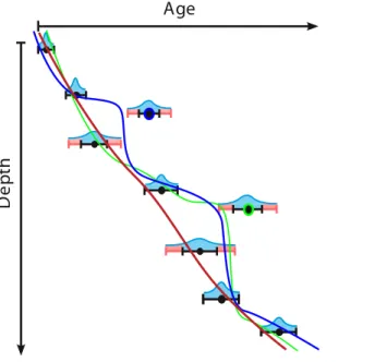
Here, we classify all reversals into two types: tractable and non-tractable. In the MC simulations (which are at the heart of COPRA) these two classes of reversals have

different properties. A non-tractable reversal is said to be present if the considered

error intervals of the two involved dated points do not overlap; otherwise the reversal

is tractable (Fig. 2). More formally, a non-tractable reversal has its lower 2σ margin

5

outside the upper 2σ margin of the subsequent dated point: T_i−2σ_iT > T_i₊1+2σ

T i+1.

For a tractable, or benign, reversal, the lower 2σ margin of the dated point is smaller

than the upper 2σ margin of the subsequent dating point, thus the error intervals are

overlapping and ensure that the negative slope can be compensated within the error bounds: so although we findT_i > T_i₊₁, the ages and their errors satisfyT_i−2σ_iT ≤T_i₊₁+

10

2σ_iT₊₁.

A tractable reversal in the input data does not need correction for the Monte-Carlo approach to yield a result in finite time. Conversely, a non-tractable reversal will have to be “treated” by the user in an appropriate way, otherwise the algorithm will not converge to a final result in a reasonable amount of time.

15

2.3.3 Treatment of outliers and reversals

If a date causes a tractable reversal, a “bottleneck” in the age–depth plot for

Monte-Carlo simulation, COPRA will highlight the suspicious date (ti+1), and suggest further

inspection and treatment. A non-tractable reversal will require the user to inspect the dating table and modify it before it can begin modeling the age–depth relationship. It is

20

important to note that while our algorithm will highlight one point of the dating table for a reversal, the dates right before and after this point might just as well be erroneous instead. Thus, treating the adjacent dated points could also lead to a consistent growth

history and the final set of dates is the experts choice. COPRA offers two treatment

options: (a) removing the dating samples, or (b) increasing the uncertainty for desired

25

(14)

CPD

8, 2369–2408, 2012

models (COPRA)

Title Page

Tables Figures

◭ ◮

Back Close

Full Screen / Esc

Discussion

P

a

per

|

Dis

cussion

P

a

per

|

Discussion

P

a

per

|

Discussio

n

P

a

per

|

2.4 Hiatuses

A hiatus is a growth interruption in the archive. Climatic changes, such as aridity, cool-ing, or biologic changes can force hiatuses, but also factors unrelated to the climate history, such as burial of stalagmites under sediment could be relevant. Therefore, their close investigation is important for reconstructing the growth history and the causes for

5

their occurrence. In stalagmites, hiatuses occur if the supply of drip water,

supersat-urated with respect to CaCO₃, ceases. Often, this points to dry conditions above the

cave, and can in itself be a “drought indicator”. Even “negative growth” can occur if un-dersaturated water dissolves the stalagmite (Lachniet, 2009). In a worst case scenario this leads to the destruction of the stalagmite, but if undersaturated water enters the

10

cave on a seasonal scale it might also lead to “micro-hiatuses”, lasting only weeks or months. The former extreme case might be rather unique and such samples are not used as palaeoclimate archives. The latter might occur undetected, and changing drip

water saturation and chemistry can potentially affect the geochemistry by re-mobilizing

uranium isotopes that can go undetected in the field.

15

Hiatuses are not unique to stalagmites. Similar effects can be observed in

low-accumulation ice cores, when strong winds can stimulate loss of accumulated snow mass (Mosely-Thompson et al., 2001).

In COPRA, hiatuses are evaluated in the context of the individual slopes∆T/∆D of

the originally given dates to depth data. A statistical test is conducted to check whether

20

the observed slope between two successive dated points is significantly lower (or zero) than in the rest of the record. If this is the case, the user can choose whether to split the age model at this point (thereby no dates are assigned between the bounds of the hiatus) and the age model is broken into segments. Alternatively, the user can again remove points or increase error margins surrounding the hiatus. If COPRA fails

25

(15)

CPD

8, 2369–2408, 2012

models (COPRA)

Title Page

Tables Figures

◭ ◮

Back Close

Full Screen / Esc

Discussion

P

a

per

|

Dis

cussion

P

a

per

|

Discussion

P

a

per

|

Discussio

n

P

a

per

|

subsequently. Likewise, if COPRA returns false positives and detects hiatuses where there should be none, the user can ignore this false detection.

The age model will be split at the detected hiatus and individual models will be cal-culated for each segment. Within each segment, the modeling extrapolates between the closest dated point and the respective hiatus depth. The user can choose to

ei-5

ther enter a known depth for any hiatus, or let COPRA use the mid-point between the bracketed dating point as the splitting depth.

2.5 Incorporating incremental dating

As discussed before in Sect. 2.1, several palaeoclimatic archives also have the capacity to provide incremental dating information such as layer counting. Typically, this

infor-10

mation is in the form of{dj,tj,σjd},j=1,. . .,n. Such a dataset is obtained by counting

N0 times (say) the depths ˆdj at which the age tj occurs; and then dj and σjd are the

mean and standard deviation of theN0dˆj observations for the age tj. Note here that

the depth scaled_j (wherej=1,. . .,n) might be quite different from the depth scaleD_i

(i =1,. . .,N) mentioned in Sect. 2.2.

15

Within the COPRA methodology we put forth a unique way to incorporate such in-formation so that we step closer to a more realistic age model in the end involving as much information as possible in its construction. Due to the absence of any well-founded methodology to achieve this, we adopt the following simple heuristic approach. First, we assume that incremental dating (layer counting) and point estimates

(U-20

series dating) are independent experiments, especially in the sense that the errors of measurement of the incremental dating points are not correlated to the errors of measurement of the point estimates. Also, we assume that since incremental dating is a relative dating technique and that the ages refer to the first dated point in the table, the age of that first incrementally dated point is zero.

(16)

CPD

8, 2369–2408, 2012

models (COPRA)

Title Page

Tables Figures

◭ ◮

Back Close

Full Screen / Esc

Discussion

P

a

per

|

Dis

cussion

P

a

per

|

Discussion

P

a

per

|

Discussio

n

P

a

per

|

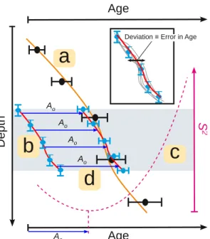
Considering the hypothetical example shown in Fig. 3 (for illustrative purposes) where layer counted age information is available in the light gray shaded area we carry out the following steps:

1. We run a Monte Carlo simulation of the point estimates alone and obtain an age model as one would have if the incremental dating information had not been there.

5

Let us call this Age Model A (the brown curve in Fig. 3a).

2. Next, we run a second Monte Carlo simulation (analogous to the description in Sect. 2.2) of the incremental dating points alone but this time by drawing random numbers from the depth axis instead of the age axis as in the previous step. The standard deviation of all realizations at any given depth then shall be the error

10

in age for that particular depth (Fig. 3, inset). Thus, by estimating the respective

means ¯t_j and deviations σ_jt¯ at all d_j, we obtain a second age model (say Age

Model B) which starts at age zero (red curve, Fig. 3b); and where the earlier error of the depths are now “transferred” to the ages, to give us{d_j, ¯t_j,σ_jt¯}.

3. The next step is to position Age Model B as optimally as possible within the

con-15

text of Age Model A. To do this, we minimize the least squares separation between

Age Model A and Age Model B (S2, dashed magenta curve, Fig. 3c) which

es-sentially means minimizing the overall distance (on the age axis) between the red and brown curves by shifting the red curve left and right. This gives us the age

offsetAo by which Age Model B has to be shifted in order to be closest to Age

20

Model A.

4. We now shift Age Model B by the vectorAo(Fig. 3d). This would transform every

point in Age Model B{d_j, ¯t_j,σ_jt¯}to{d_j, ¯t_j+Ao,σ ¯ t

j}. This allows us to construct a

fi-nal dating table combining all the depth-age information from the point estimates {D_i,T_i,σ_iT}and the age-shifted incremental dating information{d_j, ¯t_j+Ao,σ

¯ t j}. We

25

arrange the combined set{D_i,d_j}in ascending order (while keeping track of their

(17)

CPD

8, 2369–2408, 2012

models (COPRA)

Title Page

Tables Figures

◭ ◮

Back Close

Full Screen / Esc

Discussion

P

a

per

|

Dis

cussion

P

a

per

|

Discussion

P

a

per

|

Discussio

n

P

a

per

|

5. Using this combined dating table we carry out a final Monte Carlo simulation to get the final age model that incorporates dating information from both the point estimates and the incrementally dated points (not shown in Fig. 3).

The fundamental idea in this approach is that the incrementally dated points have to be first positioned in the right place within the point estimate dating table so that the

5

relative dating information stored in them can be used to construct a better age model. Minimizing the least squares separation between the two independent age models A and B provides an intuitive way to achieve this. Another point to note here is that the

shifting of the incrementally dated points by a constant ageAodoes not effect its error

as the standard deviation is invariant under a shifting constant.

10

3 Application of COPRA

In order to demonstrate the performance of COPRA, we discuss three different

scenar-ios. First, a hypothetical dataset is employed that simulates minor and major outliers (here: tractable and non-tractable age reversals) and hiatuses. Second, we test CO-PRA on a real-world stalagmite for its performance to detect and handle outliers and

15

hiatuses. Finally, we use a fast-growing, well U-series dated, and partly layer counted stalagmite to exemplify the inclusion of layer counting as a way to improve the confi-dence interval for the age model.

3.1 Data

3.1.1 Hypothetical dataset

20

(18)

CPD

8, 2369–2408, 2012

models (COPRA)

Title Page

Tables Figures

◭ ◮

Back Close

Full Screen / Esc

Discussion

P

a

per

|

Dis

cussion

P

a

per

|

Discussion

P

a

per

|

Discussio

n

P

a

per

|

We assume that a 1 m long stalagmite was obtained and ten point age estimates are spaced equidistantly along the records depth. From these depth intervals we translate into age intervals by drawing average growth rates from a uniform distribution varying

between 0.5–1.5 mm yr−1. Cumulative summing of these age intervals gives us the

ages for the dating table. To test COPRA’s abilities with respect to outliers and hiatuses

5

we modify the randomly selected growth rates to yield low or even negative increments (for outliers) or a very large age increase at low depth gain (to simulate a hiatus).

Five hundred “proxy measurements” were obtained along the 1 m long record from the top down to shortly below the maximal dating depth. A true age was assigned to these measurements by interpolation to the growth history in the dating table, taking

10

note of hiatuses, but not of outliers or reversals. The proxy signal we used was a slowly varying sinusoid with a period of 150 yr.

Synthetic layer counting data was generated for the consistent growth history case. We assumed that 25 yr from the top of the record could be counted, with a minimum error of 1 mm at the top and an additional term increasing with 1 % of layer counting

15

depth.

3.1.2 Stalagmite TSAL-1

As a real-world example, we select stalagmite TSAL-1 from Tksaltubo Cave in the Georgian Caucasus mountains that includes several outliers and a hiatus. This sample was found broken in the cave and tested for its usefulness as palaeoclimate proxy

20

archive by preliminary U-series dating and low resolution stable isotope sampling. 12 U-series dates have been measured on a multi-collector inductively coupled plasma

mass spectrometer at the University of Minnesota. 183 stable isotope samples (δ18O)

have been measured at the ETH Zurich at 2 mm intervals as a reconnaissance profile. The ca. 360 mm long TSAL-1 grew between 46 and 35.5 kyr BP. The lowermost age

25

shows large errors, due to contamination in the laboratory.

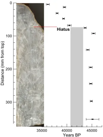
TSAL-1 features a visible growth interruption at a depth of 72.5±0.2 mm (Fig. 4).

(19)

CPD

8, 2369–2408, 2012

models (COPRA)

Title Page

Tables Figures

◭ ◮

Back Close

Full Screen / Esc

Discussion

P

a

per

|

Dis

cussion

P

a

per

|

Discussion

P

a

per

|

Discussio

n

P

a

per

|

submergence of the cave, or burial of the stalagmite in sediment. The latter factor is evidenced by silt material ingrown along the sides of the stalagmite during the hiatus, whereas the hiatus surface seems to have been washed clean of sediment by drip water. The hiatus is clearly visible in the stalagmites petrography, but it can also be seen in a rather strong change in growth rate. However, without the petrographic evidence,

5

we would not be able to securely assign a hiatus. Luckily, we can measure the hiatus depth and use it as input for COPRA to split the age model into two segments.

3.1.3 Stalagmite YOK-G

As a second test on a real sample, we use a fast growing stalagmite from Yok Balum Cave, Toledo District, Southern Belize. Stalagmite YOK-G (Fig. 5), collected in 2006,

10

is an aragonite sample (confirmed by X-ray diffraction analysis) that displays visual

growth laminations of altering dark compact and milky white, more porous material. Preliminary U-series dates and layer counts suggest that the sample was fast

grow-ing (growth rate between 0.12 and 1.63 mm yr−1) and for the most part annually

lami-nated. Furthermore, environmental monitoring of Yok Balum cave supports the notion

15

that seasonal changes in dripwater chemistry and cave environment cause changes in crystal arrangement and therefore annual fabric laminations. Details on the palaeo-climatic information from YOK-G will be published in later contributions. A short layer counted interval shows fairly good agreement with U-series dating results (see Fig. 5).

3.2 Results

20

3.2.1 Hypothetical dataset

(20)

CPD

8, 2369–2408, 2012

models (COPRA)

Title Page

Tables Figures

◭ ◮

Back Close

Full Screen / Esc

Discussion

P

a

per

|

Dis

cussion

P

a

per

|

Discussion

P

a

per

|

Discussio

n

P

a

per

|

For this simulated, piecewise linearly grown, stalagmite we found the age–depth relationship without prior modification of the dating table (Fig. 6a) and the minima and maxima of the hypothetical record was determined. The proxy signal, a sinusoid with a period of 150 yr, varies slowly compared to the average sampling rate, however. For a signal with higher frequency variability it would be impossible to characterize minima,

5

maxima and change-points with confidence. The confidence intervals of the final age model, as well as the proxy time series, can be significantly narrowed if layer counting data is available, as the insets in Fig. 6 reveal.

If age reversals are deliberately embedded into the dating table they are faithfully detected and highlighted. Removing these false point age estimates leads to an age–

10

depth relationship and proxy time series consistent with the true curve (results not shown).

Unrecognized and unaccounted hiatuses can lead to erroneously narrow confidence bands in the hiatus area of the age–depth relationship and the proxy time series. On the other hand, if the hiatus is compensated by splitting the age model simulation (allowing

15

for a non-continuous age–depth relationship) the error margins before and after the period of slowed growth widen and no ages are assigned to the period in-between (results not shown).

3.2.2 Stalagmite TSAL-1

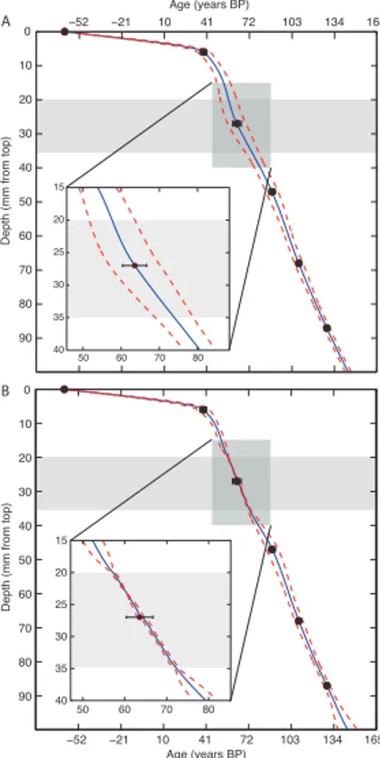
Outliers and Reversals 20

In a first step, COPRA evaluates the input data and properly detects and marks (with violet circles) two reversals (Fig. 7). When we inspect the depth-age diagram, TSAL-1 shows two seemingly suspicious samples, because they do not easily fit into a monotonous age–depth plot. The two detected reversals are caused by non-tractable reversals, which are in fact outliers, and must now be eliminated from further analysis.

(21)

CPD

8, 2369–2408, 2012

models (COPRA)

Title Page

Tables Figures

◭ ◮

Back Close

Full Screen / Esc

Discussion

P

a

per

|

Dis

cussion

P

a

per

|

Discussion

P

a

per

|

Discussio

n

P

a

per

|

Hiatus

Since we know the depth of the hiatus in TSAL-1, we enter the depth when asked by COPRA in the hiatus detection and treatment loop. The age modeling is split into two compartments, and each age model segment is extrapolated from the nearest dating point towards the hiatus. Figure 8a shows the result of an untreated hiatus, while Fig. 8b

5

shows a split MC simulation with the hiatus shown as dashed line. In the continuous age model a very strong (and unlikely) decrease in growth rate is apparent, while in the split simulation two separate MC simulations are run, each extrapolating from the closest U-series date to the given hiatus depth. The realizations tend to fan out near the hiatus, as they do at the base and top of the stalagmite.

10

The proxy time series for TSAL-1 on an absolute time scale is obtained as the final output of COPRA (Fig. 9). While the older segment of TSAL-1 shows a trend towards more positive values, with rather large uncertainties, the younger segment above the hiatus reflects some clear variations. The confidence interval indicates how well (or

not) these variations inδ18O can be interpreted in a palaeoclimatic context.

15

If we use a simple interpolation of the U-series dates to the depth scale of TSAL-1 instead considering the absolute time scale and dating uncertainties, the resulting proxy record shows remarkable variations and might prompt to unwarranted conclu-sions about high-frequency fluctuations (Fig. 9). COPRA allows a more reliable as-sessment of such variations.

20

3.2.3 Stalagmite YOK-G

We use the presence of both U/Th dates as well as layer counted (relative) age

infor-mation in the case of the stalagmite YOK-G in order to test the efficiency of the COPRA

methodology in effectively incorporating the layer counted ages to increase our

confi-dence in the proxy record. The age model for YOK-G is fairly linear (beyond the second

25

(22)

CPD

8, 2369–2408, 2012

models (COPRA)

Title Page

Tables Figures

◭ ◮

Back Close

Full Screen / Esc

Discussion

P

a

per

|

Dis

cussion

P

a

per

|

Discussion

P

a

per

|

Discussio

n

P

a

per

|

because this reduced uncertainty is also reflected in a reduced uncertainty of the proxy values: higher frequency variations remain interpretable (Fig. 11b) whereas the proxy record obtained without the layer counted information fails to capture any of the higher frequency variations in the same age interval (Fig. 11a).

4 Discussion

5

4.1 Proof-of-concept

The results shown in Sect. 3.2.1 present a simple but powerful proof-of-concept for the COPRA methodology. COPRA manages to estimate the proxy record and the varia-tions within it to reasonable accuracy. We would like to note here that, apart from the basic assumptions that were highlighted in Sect. 2.1, COPRA is not restricted to any

10

particular model of growth or sediment accumulation. In the current version of COPRA, a Monte Carlo simulation is used to estimate confidence intervals for the ages, based on Gaussian distributed dating errors. This step can be replaced by other methods es-timating the confidence intervals, e.g. by Bayesian techniques, which might also allow for considering other age distributions (e.g. as evident for radiocarbon ages, Blaauw,

15

2010). COPRA is a general information-content-based approach that is limited only by the accuracy of the measurements provided. This is further supported by the fact that it is able to give a better estimate (closer to the true value) as well as a narrower con-fidence bound when additional information (in the form of layer counts) is provided (cf. Fig. 6).

20

(23)

CPD

8, 2369–2408, 2012

models (COPRA)

Title Page

Tables Figures

◭ ◮

Back Close

Full Screen / Esc

Discussion

P

a

per

|

Dis

cussion

P

a

per

|

Discussion

P

a

per

|

Discussio

n

P

a

per

|

4.2 Managing outliers and hiatuses effectively

The real-world examples in Sects. 3.2.2 and 3.2.3 represent different practical

prob-lems when developing age models for proxy climate records: outliers, age reversals and hiatuses. COPRA is able to detect tractable and untractable reversals, but is also

flexible enough to treat reversals and outliers differently when appropriate based on

5

additional information. It also allows the user to exclude any other problematic dating point that the specialist might be aware of due to independent information relating to the experiment. Furthermore, hiatuses can be either defined manually (if the hiatus depth is known), or detected automatically by COPRA. On detecting a hiatus, the age model can be split into segments (above and below the hiatus) and the age model in

10

each segment is calculated individually (cf. Fig. 8). If a hiatus is assigned automatically COPRA uses the mid-point between the bracketing dates, as no direct hiatus depth is known. This method of dealing with a hiatus is realistic and relevant to the actual growth of the stalagmite because the proxy record does not attribute any proxy values to the hiatus period (Fig. 9). If the age modeling had not been split into two independent

15

segments at the hiatus then there would have been a proxy estimate inside the hiatus years with very narrow confidence bounds, which is both meaningless and false.

4.3 Layer counts increase accuracy

An algorithm to combine layer counting information with point-wise dating improves the confidence intervals for the counted segment of the age model. However, to date,

20

a method for combining incremental dating information along with point-wise dating was lacking. This feature in COPRA is thus a significant advancement, as it allows the

construction of reliable age models even if individual dates (be it U-series or14C dates)

show rather large uncertainties.

Furthermore, the increase in accuracy of the age model within the layer counted

25

interval can yield drastic differences in the proxy record (Fig. 11). The region that the

(24)

CPD

8, 2369–2408, 2012

models (COPRA)

Title Page

Tables Figures

◭ ◮

Back Close

Full Screen / Esc

Discussion

P

a

per

|

Dis

cussion

P

a

per

|

Discussion

P

a

per

|

Discussio

n

P

a

per

|

the layer counted data, whereas it revealed several oscillations in the climate proxy in the same interval as soon as the layer counts were included in the estimation process.

4.4 An “absolute” time scale for all proxies

With COPRA we introduce the concept of a true, absolute time scale. When

com-paring different proxy records from different places that are also differently dated, it is

5

important to have the same, common time scale for all these records, like a reference system in a physical experiment. As the time can be considered as an absolute

vari-able in a physical sense (at least when we do not consider relativistic effects), the time

is the only reference system that can be used as the common reference for the proxy records.

10

Using this concept, instead of asking when a certain range in the sediment was deposited, we ask what is the most likely deposited sediment range (depth) that was deposited at a certain (true and absolute) year. Following this idea, COPRA is able to provide a new time series of the proxy record where the probability distributions of the proxy values are assigned to the true dates, the absolute time scale, allowing for

15

comparability of differently dated proxy records.

The distribution of the ages (generated from the MC run) is used to transfer the age uncertainties into uncertainties of the proxy record and to assign an absolute (true) time axis (using interpolation). Thus, for each true chronological date, a distribution of the proxy values is assigned. The median of the proxy value distribution can be further

20

used for subsequent time series analysis. The calculated confidence levels and usage of the median proxy record allow a more reliable interpretation of the proxy variation, as well as a better comparison with other proxy records.

A further interesting point to note regarding the incorporation of age uncertainties into proxy estimation is that the resultant proxy record has lesser variability than a proxy

25

(25)

CPD

8, 2369–2408, 2012

models (COPRA)

Title Page

Tables Figures

◭ ◮

Back Close

Full Screen / Esc

Discussion

P

a

per

|

Dis

cussion

P

a

per

|

Discussion

P

a

per

|

Discussio

n

P

a

per

|

taking the uncertainties of the measurements into account. That is, our knowledge of proxy variations is constrained (or, to look at it conversely, “enhanced”) by the mea-surement errors (or “precision”).

5 Conclusions

Age modeling, i.e. building a reliable chronology for palaeoclimate proxy records, is

5

a complex process and is often difficult to be objectively performed and to be reported

in sufficient detail. Moreover, different assumptions and priorities considered can

pro-duce incommensurable chronologies, thus, incomparable proxy time series. We have proposed a new algorithm for COnstructing Proxy-Record Age models (COPRA). It al-lows for a reliable and reproducible outlier definition, hiatus detection, error estimation,

10

and, for the first time, inclusion of layer counted intervals to improve overall confidence intervals.

In the future, we plan to continue the development of COPRA, e.g. for improving the outlier detection algorithm that is now based on age reversals, and hiatus detection that is challenged if the hiatus is short compared to the dating resolution. The latter is

15

especially important for chronologies with very short (sub-centennial to sub-decadal) growth interruptions that are of great importance for a realistic interpretation of climate proxy records. Moreover, depth errors (resulting from physical sampling) are not yet in-corporated in the analysis, but will be included in a future version of COPRA. Generally, these integrative errors are negligible, but with analytical improvements and reduced

20

analytical errors this physical uncertainty must be kept in mind.

COPRA is freely available at http://tocsy.pik-potsdam.de (Toolbox for Complex Sys-tems [TOCSY]). Besides the algorithmic implementation of age modeling, this software supports the user in decision-making in a user-friendly GUI-environment. Although it is

implemented for MATLAB®, the core of the software (without the GUI) can be used in

25

(26)

CPD

8, 2369–2408, 2012

models (COPRA)

Title Page

Tables Figures

◭ ◮

Back Close

Full Screen / Esc

Discussion

P

a

per

|

Dis

cussion

P

a

per

|

Discussion

P

a

per

|

Discussio

n

P

a

per

|

Appendix A

The COPRA workflow

After preparing the basic input data (dating and proxy data tables) and import of these files, the user is guided through the modeling algorithm (Fig. A1). First, the user is asked if additional information is available (e.g. layer counted segments or hiatus

in-5

formation). If no additional data is available, COPRA proceeds to check the record for age reversals. If a layer counted interval is available, the number of counted years, the lower depth, and the upper depth of the counted interval must be entered.

After these tests the user confirms the selected dating information (which is shown as an age–depth graph) and the actual modeling is initiated. In the process the user can

10

modify the interpolation routine used (polynomial, spline, cubic, or linear (default)). In the case of hiatuses, treatment selection choices must be made by the user (involving further exclusion of points, or increase of error margins, or the splitting of the simulation into two independent age models) for each hiatus detected and/or specified. Further, the number of MC simulations, the confidence interval, and the type of central estimate

15

(like median or mean) can be changed (COPRA uses 100 MC simulations, the 95 % confidence level, and the median value as center point as default).

The MC simulation is performed next and the resulting age–depth relationship with the dates and their errors, and with the chosen confidence intervals, is displayed. Sub-sequently, the user can confirm and continue (if satisfied), or repeat the process by

20

either making a different choice concerning the included dates and hiatuses, or

choos-ing different MC simulation parameters. Once the user is satisfied COPRA proceeds

with computing proxy-age relations and associated uncertainties (COPRA uses the confidence level given above for the MC simulation, by default).

Finally, the output data (proxy vs. depth or age, with vertical (proxy) and horizontal

25

(27)

CPD

8, 2369–2408, 2012

models (COPRA)

Title Page

Tables Figures

◭ ◮

Back Close

Full Screen / Esc

Discussion

P

a

per

|

Dis

cussion

P

a

per

|

Discussion

P

a

per

|

Discussio

n

P

a

per

|

as plain ASCII files. The metadata ensures repeatability using the same input data and settings.

Acknowledgements. This study was financially supported by the Schweizer National Fond (SNF), Sinergia grant CRSI22 132646/1, the German Federal Ministry of Education and Research (BMBF project PROGRESS, 03IS2191B), National Science Foundation

(HSD-5

0827305), the DFG research group HIMPAC (FOR 1380), and ERC Starting Grant 240167. Lydia Zehnder (ETH Zurich) is acknowledged for her support during X-ray diffraction analysis.

References

Blaauw, M.: Methods and code for “classical” age-modelling of radiocarbon sequences, Quat. Geochronol., 5, 512–518, 2010. 2372, 2375, 2390

10

Blaauw, M., Christen, J. A., Mauquoy, D., van der Plicht, J., and Bennett, K. D.: Testing the timing of radiocarbon-dated events between proxy archives, Holocene, 17, 283–288, 2007. 2372, 2373

Bronk Ramsey, C.: Deposition models for chronological records, Quaternary Sci. Rev., 27, 42– 60, 2008. 2373

15

Bronk Ramsey, C.: Dealing with outliers and offsets in radiocarbon dating, Radiocarbon, 51, 1023–1045, 2009. 2380

Fairchild, I. J., Smith, C. L., Baker, A., Fuller, L., Sp ¨otl, C., Mattey, D., McDermott, F., and E. I. M. F.: Modification and preservation of environmental signals in speleothems, Earth-Sci. Rev., 75, 105–153, 2006. 2376

20

Hu, C., Henderson, G. H., Huang, J., Xie, S., Sun, Y., and Johnson, K. R.: Quantification of Holocene Asian monsoon rainfall from spatially separated cave records, Earth Planet. Sc. Lett., 266, 221–232, 2008. 2372

Lachniet, M. S.: Climatic and environmental controls on speleothem oxygen-isotope values, Quaternary Sci. Rev., 285, 412–432, 2009. 2382

25

(28)

CPD

8, 2369–2408, 2012

models (COPRA)

Title Page

Tables Figures

◭ ◮

Back Close

Full Screen / Esc

Discussion

P

a

per

|

Dis

cussion

P

a

per

|

Discussion

P

a

per

|

Discussio

n

P

a

per

|

Mattey, D. P., Fairchild, I. J., Atkinson, T. C., Latin, J.-P., Ainsworth, M., and Durell, R.: Sea-sonal microclimate control of calcite fabrics, stable isotopes and trace elements in modern speleothem from St Michaels Cave, Gibraltar, Earth-Sci. Rev., 75, 105–153, 2006. 2376 Medina-Elizalde, M. and Rohling, E. J.: Collapse of classic Maya civilization related to modest

reduction in precipitation, Science, 335, 956–959, 2012. 2372

5

Mosley-Thompson, E., McConnell, J. R., Bales, R. C., Lin, P.-N., Steffen, K., Thompson, L. G., Edwards, R., and Bathke, D.: Local to regional-scale variability of annual net accumulation on the Greenland ice sheet from PARCA cores, J. Geophys. Res., 106, 33839–33851, 2001. 2382

Preunkert, S., Wagenbach, D., Legrand, M., and Vincent, C.: Col du D ˆome (Mt Blanc Massif,

10

French Alps) suitability for ice-core studies in relation with past atmospheric chemistry over Europe, Tellus B, 52, 993–1012, 2000. 2376

Rehfeld, K., Marwan, N., Heitzig, J., and Kurths, J.: Comparison of correlation analysis tech-niques for irregularly sampled time series, Nonlin. Processes Geophys., 18, 389–404, doi:10.5194/npg-18-389-2011, 2011. 2372

15

Scholz, D. and Hoffmann, D.: StalAge – an algorithm designed for construction of speleothem age models, Quat. Geochronol., 6, 369–382, 2011. 2372, 2373

Svensson, A., Andersen, K. K., Bigler, M., Clausen, H. B., Dahl-Jensen, D., Davies, S. M., Johnsen, S. J., Muscheler, R., Parrenin, F., Rasmussen, S. O., R ¨othlisberger, R., Seier-stad, I., Steffensen, J. P., and Vinther, B. M.: A 60 000 year Greenland stratigraphic ice core

20

chronology, Clim. Past, 4, 47–57, doi:10.5194/cp-4-47-2008, 2008. 2376

Telford, R. J., Heegaard, E., and Birks, H. J. B.: All age–depth models are wrong; but how badly?, Quaternary Sci. Rev., 23, 1–5, 2004. 2371

Treble, P. C., Chappell, J., and Shelley, J. M. G.: Complex speleothem growth processes revealed by trace element mapping and scanning electron microscopy of annual layers,

25

Geochim. Cosmochim. Acta, 69, 4855–4863, 2005. 2376

(29)