The use of Bayesian Networks in Detecting the States of Ventilation Mills in Power Plants



Abstract—The main objective of this paper is to present a new method of predictive maintenance which can detect the states of coal grinding mills in thermal power plants using Bayesian networks. Several possible structures of Bayesian networks are proposed for solving this problem and one of them is implemented and tested on an actual system. This method uses acoustic signals and statistical signal pre-processing tools to compute the inputs of the Bayesian network. After that the network is trained and tested using signals measured in the vicinity of the mill in the period of 2 months. The goal of this algorithm is to increase the efficiency of the coal grinding process and reduce the maintenance cost by eliminating the unnecessary maintenance checks of the system

Index Terms—_{Acoustic Signals, Bayesian Networks, Predictive} Maintenance, Ventilation Mills.

Original Research Paper DOI: 10.7251/ELS1418016V

I. INTRODUCTION

ONDITION based maintenance (CBM) is a maintenance technique widely used in the industry today. It uses data collected through condition monitoring to advise whether maintenance is necessary, and thus reduces maintenance cost of the system [1]. Many of the maintenance techniques that are currently implemented are using a certain type of time-based preventive maintenance, where the components of the system are checked regularly after a certain period of time to ensure that no serious fault has occurred. This kind of maintenance is being conducted on ventilation mills in thermal power plants where, due to the inability to predict the state of the coal grinding plate within the mill, the entire subsystem needs to be periodically stopped and inspected. This paper proposes a new method of predictive maintenance which can detect the state of the plates within the mills based on the acoustic signals

Manuscript received 13 April 2014. Accepted for publication 30 May 2014.

S. Vujnović is with the School of Electrical Engineering, University of

Belgrade, Belgrade, Serbia (phone: +381-11-3218-370; e-mail: svujnovic@etf.bg.ac.rs).

P. Todorov is with the School of Electrical Engineering, University of Belgrade, Belgrade, Serbia (e-mail: pedjatodorov@etf.bg.ac.rs).

Ž. Đurović is with the School of Electrical Engineering, University of

Belgrade, Belgrade, Serbia (e-mail: zdjurovic@etf.bg.ac.rs).

A. Marjanović is with the School of Electrical Engineering, University of

Belgrade, Belgrade, Serbia (e-mail: amarjanovic@etf.bg.ac.rs).

measured in the vicinity of the mill, using Bayesian networks (BN).

Bayesian networks have been widely used for the purpose of predictive maintenance in the last few years. Since their introduction in the mid 80’s [2] they have experienced a rapid development in many areas of research. Also, due to their ability to represent complex systems in which high amount of uncertainty exists, they have proven themselves to be superior to other methods such as neural networks, support vector machines, etc. In this paper several BN structures will be proposed which serve to model the states and the behaviors of ventilation mills, and one of them will be tested on actual acoustic measurements.

There are many examples of fault detection algorithms which are based on the measurements of vibration signals of the machines ([3] and [4], to name a few). However, it has long since been shown that acoustic measurements can be as informative as vibration signals when it comes to detecting the faults in machines [5]. The usage of acoustic signals in fault detection has expanded during the last decade [6], however they are still considered to be a lesser alternative to vibration signals, due to their high susceptibility to surrounding noise. In this paper acoustic signals acquired in a very noisy environment will be used to test the efficiency of a simple Bayesian network for the detection of states in the ventilation mills. More complex realizations of the solution to the problem will be proposed as well.

This paper is structured as follows. In Chapter 2 a short introduction to Bayesian Networks is presented, while in Chapter 3 some practical realizations of BNs which can be used for fault detection are proposed. Chapter 4 describes the system on which the algorithms have been tested, as well as the process of acquiring acoustic signals. In Chapter 5 the results of the algorithm are presented and in Chapter 6 the final conclusions to this paper are stated.

II. BAYESIAN BELIEF NETWORKS

Bayesian Belief Network (BBN) is a term introduced in 1980s by Jude Pearl [2] in an attempt to create a mathematical probabilistic tool capable of modeling and reproducing the process of human reasoning. The basic idea was to reproduce the way in which people accumulate information from different sources and use it to develop conclusions about certain ideas. During the last decade Bayesian networks have become a very powerful tool for representation of complex

The use of Bayesian Networks in Detecting the

States of Ventilation Mills in Power Plants

Sanja Vujnovi

ć

, Predrag Todorov,

Željko Đurović, and Aleksandra Marjanović

C

systems and it has been used in many areas of research including fault detection and fault isolation [7], [8].

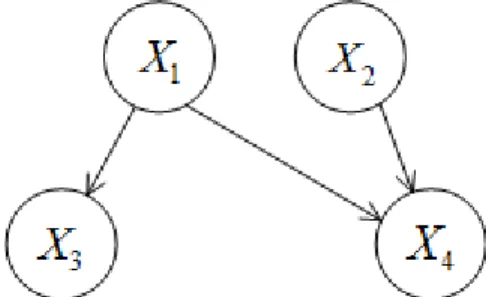
Fig. 1. A simple Bayesian network which consists of 4 nodes (X1, X2, X3 and X4) and three connections between them.

A. Bayesian Theorem

Bayesian networks apply Bayesian theorem on complex systems to calculate conditional probabilities of certain events or hypothesis when a new evidence is obtained. Bayesian theorem was coined by Thomas Bayes in the 18th century and it can be formulated as

_. ) ( ) | ( ) ( ) | ( E P H E P H P E H

P n n

n  (1)

Here P H( _n|E) is a posterior probability of hypothesis

Hn when evidence E is known. P H( _n) and P E( ) are prior probabilities of hypothesis and evidence, respectively, and

( | _n)

P E H is the probability of evidence E given the hypothesis H_n. The great advantage of Bayes' theorem is that it allows us to easily calculate conditional probabilities based on the corresponding prior probabilities. In this case, if H_n is, for example, a certain fault, and E is evidence or a symptom of a fault, than P H( _n) and P E H( | _n) can be more easily obtained from the survey or maintenance data, than the conditional probability of a fault given the evidence.

If we assume that i denotes a specific hypothesisH_i, then (1) can be rewritten using the rule of total probability, where the summation is taken over all hypotheses H_i which are mutually exclusive and their prior probabilities sum up to 1. The final form is given as

_. ) | ( ) ( ) | ( ) ( ) | (



i i i

n n n H E P H P H E P H P E H P (2)

This is called inference and it represents the basic idea of how the inserted evidence spreads throughout Bayesian networks.

B. Topology of Bayesian Network

Bayesian network is an acyclic probabilistic graph which contains a set of nodes and directed connections between them and it is used to represent the knowledge about uncertain

events. Nods represent the probabilistic variables which can be continuous or discrete. Connections between nodes represent the probabilistic dependencies among certain variables. A simple type of Bayesian network is shown in Fig. 1. Here an edge from node X1 to node X3 and from nodes X1 and X2 to node X4 represent a statistical dependence between the corresponding variables. Therefore a value taken by a variable X4 depends on the values taken by variables X1 and X2. Nodes X1 and X2 are then referred to as the parents of X4 and, similarly, X4 is referred to as the child of X1 and X2. In general, for the network with n nodes: X1, X2,..., Xn, the joint probability can be expressed as

1 2

1

( , ,..., ) ( | ( )) ,

n

n i i

i

P X X X P X pa X







where pa X( _i) is a set of parents of the node X_i.

There are many types of nodes which can be chosen for any given Bayesian network. However, in practice only two types of variables are used: discrete and continuous Gaussian. This is because only for these two types of nodes can the exact computation of conditional probabilities be done [9]. Similarly, the discrete variables cannot have continuous parents if the exact computation is required. Therefore, there are three different combinations of nodes for the parent-child relationship and three different methods for calculating conditional probabilities. If discrete variables have discrete parents, their conditional probabilities are expressed via conditional probability table. For example, if both X1 and X3 from Fig. 1 are discrete variables, with n and m different possible states respectively, their conditional probability table would have n x m entries of conditional probabilities

3 3 1 1

( _i| _k)

P X x X x , where x_3i is the i-th state of node X3 and x_1k the k-th state of the node X1. On the other hand, if X3 was a Gaussian continuous variable and X1 its discrete parent, the conditional probability distribution would be Gaussian as well [9].

C. The Learning Process

There are two ways of calculating parameters of Bayesian network, as well as the structure. One is based on an expert knowledge of the system and the other on machine learning using experimental results. These two approaches can be used jointly or individually.

Assuming that the expert knowledge of the system is unavailable and that Bayesian network needs to be taught its structure and parameters, there are several ways in which this can be achieved. Structure learning itself is much more complicated than the parameter learning and we will not dwell on it further in this paper. For all intents and purposes we will assume that the structure of the Bayesian network is known and that only the parameters need to be taught.

In the case when all the nodes (variables) of the system are observable, the most common algorithm for machine learning of the Bayesian network is the log likelihood approach. Here

the goal is to learn all of the conditional probability densities which maximize the likelihood of the training data. That is to

Fig. 2. Bayesian network with one measured continuous node (X3), one hidden discrete node (X2) and one discrete node which represents the state of impact plates and which cannot be directly measured (X1).

say that if we have Bayesian network B( , )S p with defined structure S and parameters p, and where D is a set of training data with the values of all the parameters p of network B, then the goal is to maximize the likelihood, i.e. the probability of the data d given the Bayesian network B:

_{( | ) ,} d D

L P d B







or as it is more commonly expressed in logarithmic form: _{log ( | ).}

2



 

D d

B d P

LL (5)

If by any chance there is a choice of several Bayesian network models, it is wise to adopt the model which gives the maximum likelihood given the data obtained.

Usually however, not all the parameters can be measured, and some connections between the nodes must be modeled with unobservable variables. In such cases the exact log likelihood approach cannot be used and the approximate parameter estimation must be conducted. The most popular approximate algorithm for teaching the Bayesian network with hidden nodes is the Expectations maximization (EM) algorithm. This algorithm consists of two steps. In the first step, called the expectation step, the current parameter estimations pˆ are used to calculate expectations for the missing values of hidden variables. Then, in the second step called the maximization step, a new maximum likelihood estimate of the parameters is calculated after which the algorithm goes back to the previous step. This continues throughout the entire training set.

III. APPLICATION OF BAYESIAN NETWORK IN PREDICTIVE MAINTENANCE

The fundamental problem with Bayesian networks is deciding which model adequately represents the system which

is observed. First of all, the variables used in the system need

to be chosen. They can represent some physical, measurable property of the system or some unknown interference which

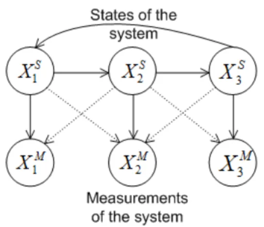
Fig. 3. Hidden Markov model represented with Bayesian networks. XiS are the states of the system and XiM are the measurements of the system. All the variables are continuous Gaussian and visible.

cannot be measured. Then, the decision needs to be made concerning the type of the chosen variables. They can be discrete or continuous, visible or hidden. Secondly, the question of the structure of the Bayesian network should be decided upon. This is the most important and the most complex question. The types of structures which can be represented with Bayesian networks are vast, and the only limit one faces when choosingthem is the knowledge of the causal relationships within the physical system and the complexity sufficient to solve the given problem. In this chapter several structures will be proposed for solving the problem of detecting the states of ventilation mills.

A. The Simple Static Model

The simplest Bayesian network that can be used for detecting the state of the mill is shown in Fig. 1. Circles represent continuous-valued random variables, squares are discrete random variables, clear boxes represent observed nodes and gray boxes represent hidden nodes. This network contains only 3 nodes (variables), two of which are discrete and one of which is continuous Gaussian.

The basic idea is that the measurements taken outside of the mill are directly influenced by the state of the impact plates within the mill and by a hidden variable which is modeled as a discrete node. This hidden, immeasurable node can represent an outside noise, unknown component of the system or some other feature which does not necessarily need to have a physical interpretation. The state of the plates X1 is modeled as a discrete node with 2 states: healthy plates and worn plates. The measured signal which is represented by the node X3 is a two-dimensional Gaussian variable.

B. Hidden Markov Model

Hidden Markov model (HMM) can be modeled as a simple dynamic Bayesian network, where the next state of the system depends on the previous state and the state transition probabilities, and where the states themselves are not directly measured. However, even though the states cannot be

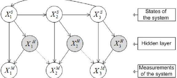
Fig. 4. Complex dynamical BN model. XiS are the states of the system, XiM are the measurements of the system and XiH. are the hidden variables of the system which cannot be observed or detected. All the nodes are continuous and Gaussian.

measured, they influence the measurements of the system which are then used to infer the state in which the system is in. Hidden Markov models are used for a very broad range of systems and one such model (Fig. 3) can be used to infer the states of the impact plates in ventilation mills.

In Fig. 3, XiS represents a state node and XiM a measurement node. All of the variables are chosen to be continuous and visible (that is to say, information on states and measurements can be used when training the network). In this case 3 continuous states are chosen: the state of healthy plates (X1S ), the state when the plates are used but not damaged enough, so the repair is not necessary (X2S ) and the state which represents worn plates (X3S ) and which indicates that the repair should be done as soon as possible.

Note that the transition between states is modeled so that the state deteriorates up until a point when the plates have to be replaced, and only then can the state return to the initial value of healthy plates. Also, each state influences the appropriate measurement of the system, but due to noise and inconsistencies it can appear as a measurement of the adjacent state as well (presented by dotted lines in Fig. 3).

A. The Complex Dynamical Model

As we have noted, HMM are broadly used to model all sorts of systems in many areas of research. However, they represent only a simple usage of dynamic Bayesian network which can easily be modified to include more complex demands of the system. One such modification is proposed in Fig 4, where the mixture of first two solutions to Bayesian network models is implemented. Here the one-way transition between the states is included as well as the influence of the unknown, hidden variable on the measurements of the system.

IV. CASE STUDY

In the previous chapter some possible structures of Bayesian networks were proposed that can be used for predictive maintenance. The actual process on which one of these solutions will be tested is a ventilation mill in thermal power

plant Kostolac A (Serbia) and it will be described in this chapter. Also, the process of acquiring and pre-processing of acoustic signals used in simulations will be depicted.

A. Ventilation Mill

Coal grinding mills are a very important subsystem of thermal power plants. Their main purpose is to pulverize the coal into fine powder before it can get into the furnace. The mill itself consists of coal grinding plates (also called impact plates) which rotate within it with the frequency of fr=12.5Hz and are used to crush the coal into smaller pieces until it gets sufficiently fragmented. After that it drifts into the furnace system where it is used as a fuel.

During the grinding process the impact plates get slowly depleted and their efficiency reduces. In the early stages this causes them to pulverize the coal more slowly, but if the plates are not changed for a long period of time it can cause a complete malfunction of the milling subsystem in thermal power plants. Some algorithms for solving this problem have already been proposed [10]. Currently this problem is being solved by employing a type of time based maintenance, which implies stopping the entire subsystem once every 8 or 9 weeks, conducting visual inspection of the plates and, if it is deemed necessary, replacement of the plates with the new ones. This can be very costly if the overhaul was concluded not to be necessary.

In this paper a new algorithm will be tested which uses acoustic signals recorded in the vicinity of the mill, while the mill is operating mode, and Bayesian networks to determine the state of the impact plates, i.e. whether the replacement is necessary or not.

B. Acoustic Signals

Acoustic signals were recorded in the vicinity of the mill while it was in operating mode. The measurements were conducted every couple of weeks in the period of two months, thus encompassing the entire life cycle of the plates, from the moment they were replaced to the moment when they were completely depleted. These signals were recorded with the

sampling frequency of fs=48kHz and 24bit encryption. Approximately once every two weeks an acoustic signal has been measured, which has afterward been divided into 20-30 shorter signals.

For the training and testing of the Bayesian network the sampling period was downsized to 4.8kHz, Also, certain features were extracted from the signal which were later used in the decision making process. These features are the basic properties of the signal in time and frequency domain. Eight features in time domain are chosen as characteristic parameters of the signal [3]:

 Arithmetic mean value:

1 1

( ) N i

x x i

N 





 Root mean square value:

1/ 2 2 1 1 ( ) N rms i

x x i

N 

 

 _



 Square mean root value:

2 1/ 2 1 1 ( ) N r i

x x i

N 

 

 _



 Skewness index:





1 1

( ) /

N

ske _i v

x x i x x

N 

 

  





 Kurtosis index:





1 1

( ) 4 /

N

kur i v

x x i x x

N 

 

_  _





 C factor: CPP x/ _rms

 L factor: LPP x/ _r

 S factor: Sx_rms/x

where xv is the variance of the signal x and PP is peak-to-peak value of the signal. Also, eight features in the frequency domain were chosen as the most dominant components in the frequency spectrum of the signal, in the same way it has been done in [10]. They represent the maximum value of the amplitude frequency spectrum of the signal at the frequencies:





f  Hz.

After extracting these features a vector of 16 elements is acquired for each of the measured signals. To reduce the dimension of this vector and therefore reduce the amount of variables needed for the Bayesian network, a linear dimension reduction algorithm is applied which transforms a 16-dimentional vector X into a two-16-dimentional vector Y [11]: _{21 16}T _{2 2x1}.

x

x A X

Y  (6)

The matrix A is chosen so to minimize the loss of information by maximizing the distance of two extreme classes - the class of healthy and the class of worn plates. This matrix is acquired by maximizing the criteria ( 1 )

W B

J tr S S where

W

S is a within-class scatter matrix and S_B is a between-class scatter matrix, as defined in [11], and applied in [3]. After this procedure has been implemented, the 2-dimensional vector of features Y is used as an input to a Bayesian network.

V. RESULTS

For the testing of this algorithm the Bayesian Network depicted in Fig. 2 is used. The first variable (X1) represents the true state of the system and is chosen to be a discrete variable with two possible states - healthy and worn plates. The second variable (X2) is a hidden variable and it does not have a specific physical meaning. It represents the noise in the surroundings that can influence the measurements, as well as unknown parameters of the system that were not otherwise included in the model. It is also chosen to be a discrete variable with two possible states. Finally, the third variable (X3) represents the measured output of the system, or in this case, a parameter Y gained by signal pre-processing techniques described in the previous chapter. This variable is chosen to be continuous and Gaussian. With this in mind, the joint probability of this Bayesian network is:

P(X₁,X₂,X₃)P(X₃|X₁,X₂)P(X₂|X₁)P(X₁). (7) The idea is to calculate the probability of each of the states in X1 given the measurements X3.

Learning and testing procedures for this Bayesian network are done in a programming package Matlab, using toolbox for Bayesian networks created by [9]. For a training set, the signals taken slightly before and slightly after the change of plates were chosen, representing the two extreme states of the mill. Since there is a hidden node within the system, the EM learning algorithm is applied. The testing is done on all the signals. No initial assumptions about the conditional probabilities were made, so only after the learning process has been completed, the conditional probability table for all the nodes had been constructed. The testing has been done in two ways - real time and offline testing.

In average of every two weeks, a recording has been conducted, enabling us to acquire around 30 acoustic signals, thus giving us a complete database of a over 120 signals throughout the entire lifespan of the grinding plates. In order to test this algorithm in real time, all these signals have been artificially merged so to appear as though the seconds have passed between different measurement sessions, when indeed it has actually been weeks. However, despite the artificially created sudden changes in the state of the mill (which are realistically much slower) the algorithm tested in real-time has shown some very good results.

From Fig. 5 it can be concluded that this simple Bayesian network can successfully detect the states of the grinding plates. Two weeks after they have been changed the algorithm detects that the plates are completely healthy, 5 weeks after the change the deterioration of the plates becomes noticeable, and the Bayesian network detects 25% probability that the plates are worn. After 6 weeks this percentage increases to 50%, whereas after 8 weeks the algorithm reports with 100% certainty that the plates need to be replaced. In order to prevent sudden changes in real time testing environment, the output of the Bayesian network is averaged over the last 10 time periods (each of which lasts 15 seconds). It can be noted

Fig. 5. Results of a real-time test. Bayesian network has managed to calculate the probability for grinding plates to belong to each of the defined states, for each of the measured signals.

that a sudden change in the state of the plates cannot be detected in a very short period of time. It is needed approximately 4 minutes (15 time periods) for the algorithm to converge to the right state.

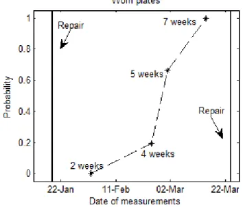
Another way of testing this algorithm, which may be more useful when taking into account the nature of the problem, is in an offline simulation. In this case the simulation has been run only after all the signals that day have been recorded. Seeing that the sudden changes in the state of the plates cannot happen, this is a more appropriate way to use this algorithm. It does not require the constant presence of the recording device which can be used once every week or so for a couple of hours to predict whether the maintenance check is necessary. The results are given in Fig. 6 and they are similar to those obtained with a real-time test.

VI. CONCLUSION

In this paper an application of Bayesian networks on predictive maintenance of ventilation mills in thermal power plants has been investigated. The basic principles of BN have been described and several solutions to the predictive maintenance problem have been proposed. Using statistical signal processing and one of the proposed structures of Bayesian networks, the algorithm has been proposed which manages to detect the state of the plates of the coal grinding mills based on acoustic signals, and therefore predict the time when it is necessary to conduct the replacement of the plates. This algorithm has been successfully tested on a real system during a time period of several months.

The final purpose of this algorithm is the development of the commercially accessible device which would be able to detect the state of ventilation mills and predict the time when it is necessary to repair them. The great advantage of this

Fig. 6. Results of offline testing. The probability that the grinding plates are damaged is calculated for each day of the measurements. The further the measurements are from the last repair the higher is the probability that the plates need to be changed.

method is that it uses acoustic signals which can be acquired without disturbing the operation of the mill. Unfortunately, this also means that the algorithm is highly susceptible to noise and acoustic disturbances. However, even with these drawbacks the algorithm developed here yields very good results despite the fact that the simplest BN model has been adopted and the measured signals had a noticeable presence of noise

In future works more complex models of Bayesian networks that include the dynamic behavior of the transition between the states of the system should be tested. Also a better database of the signals should be acquired. Finally it would be interesting to test the algorithm on acoustic signals gained with a cheaper microphone which is commercially more available.

REFERENCES

[1] A. K. S. Jardine, D. Lin, D. Banjevic, “A review on machinery diagnostics and prognostics implementing condition-based maintenance,” Mechanical Systems and Signal Processing, vol 20, pp. 1483–1510, 2006.

[2] J. Pearl, “Bayesian networks: a model of self-activated memory for

evidential reasoning,” 7th Annu. Conf. of the Cognitive Science Society, Irvine, 1985.

[3] P. Stepanic, I. V. Latinovic, Z. Djurovic, “A new approach to detection of defects in rolling element bearings based on statistical pattern

recognition,” Int J Adv Manuf Technol, vol 45, pp. 91–100, 2009. [4] S. A. McInerny, Y. Dai, “Basic vibration signal processing for fault

detection,” IEEE Transactions on Education, vol 46, no. 1, pp. 149– 156, 2003.

[5] N. Baydar, A. Ball, “A comparative study of acoustic and vibration signals in detection of gear failures using Wigner-Ville distribution,” Mechanical Systems and Signal Processing, vol 15, no. 6. pp. 1091– 1107, 2001.

[6] A. Albarbar, F. Gu, A. D. Ball, A. Starr, “Acoustic monitoring of engine

fuel injection based on adaptive filtering techniques,” Applied Acoustics, vol 71, pp. 1132–1141, 2010.

[7] Y. Zhao, F. Xiao, S. Wang, “An intelligent chiller fault detection and

diagnosis methodology using Bayesian belief nettwork,” Energy and Buildings, vol 57, pp. 278–288, 2013.

[8] S. Verron, J. Li, T. Tiplica, “Fault detection and isolation of faults in a multivariate process with Bayesian network,” Journal of Process Control, vol 20, pp. 902–911, 2010.

[9] K. P. Murphy, “Dynamic Bayesian networks: Representation, Inference

and Learning,” Ph.D. dissertation, Dept. Computer Science, Univ. of

California, Berkeley, 2002.

[10] E. Kisić, V. Petrović, S. Vujnović, Ž. Đurović, M. Ivezić, “Analysis of the condition of coal grinding mills in thermal power plants based on

the T2 multivatiate control chart applied on acoustic measurements,”

Facta Universitatis Series: Automatic Control and Robotics, vol 11, no. 2, pp. 141–151, 2012.

[11] K. Fukunaga, Introduction to Statistical Pattern Recognition. Boston: Academic Press, 1980.