A Parameter Identification Technique for
Structured Population Equations Modeling
Erythropoiesis in Dialysis Patients
Doris H. Fuertinger, Franz Kappel
Abstract—Individualization of therapy plays an increasing role in the context of chronic diseases. A model for erythro-poiesis, consisting of coupled partial differential equations, is adapted to an individual patient. The numerical approximation for the population equations is based on semigroup theory, respectively on the theory of abstract Cauchy problems. The system state is approximated by system states of high order differential equations on finite dimensional subspaces of the state space of the original system. A standard Least-Squares formulation is used to define the cost-functional used for the parameter identification. An example of (locally) well identifiable parameters expressing numerical convergence for increasing dimensions of the finite dimensional approximating system is discussed. We demonstrate that a low approximation dimension suffices to obtain accurate numerical solutions and estimates for the parameters.
Index Terms—abstract Cauchy problems, structured popula-tion equapopula-tions, erythropoiesis, chronic kidney disease, parame-ter estimation
I. INTRODUCTION
A
NEMIA effects almost all patients suffering from chronic kidney disease (CKD) and is mainly caused by a failure of renal excretory and endocrine function. Already partial correction of anemia in dialysis patients reduces cardiac-related morbidity and mortality, which is the most common cause of death among these patients (see for instance [1]–[3]). It has been suggested that chronic renal disease progression may be slower when anemia is reversed, emphasizing the benefits of early correction of the anemia with erythropoietin stimulating agents (ESA). ESAs stimulate the bone marrow to produce red blood cells, exerting a similar effect than the endogenous hormone erythropoietin (EPO) which is released by the kidneys and which is insufficiently produced in CKD patients.Erythropoiesis – the production of new red blood cells – is a very complex process. Stem cells in the bone marrow commit to the erythroid lineage and start to develop into red blood cells, so called erythrocytes. This process takes about two weeks. During this time the cells divide, differentiate and some of them eventually die. The development from stem cells into erythrocytes involves a number of different cell stages which exert diverse characteristic patterns with regard to the rate of proliferation, the rate of apoptosis, the maturation velocity and the need for EPO and other substances (for details see e.g. [4]). Therefore a model for
Manuscript submitted July 02, 2013; revised: July 31, 2013
Doris H. Fuertinger is with the Renal Research Institute, New York, NY 10065, USA, e-mail: [email protected]
Franz Kappel is with the Institute of Mathematics and Scientific Com-puting, University of Graz, Austria, e-mail: [email protected]
erythropoiesis has to include submodels for various cell pop-ulations. A rather comprehensive model for erythropoiesis was developed in [5] (see also [6]). The model presented in [5] consists of five structured population equations with cell age being the structuring attribute, two ordinary differ-ential equations describing the development of endogenous and administered EPO over time plus a number of auxiliary equations describing the influence of EPO on maturation and mortality rates and the control of EPO secretion by the kidneys based on the oxygen carrying capacity of blood which is proportional to the erythrocyte population.
In comparison to healthy persons CKD patients have a very high inter-individual variability in red blood cell (RBC) lifespan, bone marrow response to EPO, endogenous EPO production and half-life of the administered EPO compound. Routine measurements of these quantities are not practicable in a clinical environment or are simply impossible. Therefore prediction of the individual response to EPO administration schemes is extremely difficult and is further aggravated by the fact that there is a long delay in reaction of the RBC population to EPO levels. The dose and frequency of administration of an ESA treatment regimen are most often determined based on prior experience of the physician and on established guidelines. This approach bears some severe limitations so that hemoglobin levels in CKD patients tend to fluctuate widely and cycling phenomena are frequently observed, [7], [8].
Since the mathematical model developed in [5] is based on the physiological mechanisms governing erythropoiesis it can be used – as we shall show – to guide and to individualize the ESA treatment regimen for CKD patients. This requires in particular to adapt to the specific patient those model parameters which correspond to physiological quantities which are known to have a high inter-individual variability.
II. GENERALPOPULATIONEQUATION ANDNUMERICAL
APPROXIMATION
As already mentioned in the introduction the core of the model developed in [5] consists of a coupled system of five structured population equations which are of the following type:
∂
∂tu(t, x) +v(E(t)) ∂ ∂xu(t, x)
= (β−α(E(t), x))u(t, x), t≥0, x∈Ω = [xmin, xmax], u(0, x) =φ(x), x∈Ω,
v(E(t))u(t, xmin) =f(t), t≥0,
(1)
where u(t, x) is the population density at time t and cell age x. Further v(E(t)) denotes the maturation velocity of cells according to the erythropoietin level E(t)at timet, β
is the proliferation rate,α(E(t), x)the rate of apoptosis de-pending on the erythropoietin levelE(t)at timetand the cell agex. The initial population density is denoted byφ(x)and
f(t)is the influx of cells from the precedent population class at timet. The general population equation presented here, is a linear hyperbolic partial differential equation (PDE). Hyper-bolic PDEs are in general more difficult to approximate then elliptic or parabolic ones, because approximations tend to express spurious, numerically induced, oscillatory behavior. Our approach for solving the model equations numerically is based on semigroup theory respectively on the theory of abstract Cauchy problems (see e.g. [9], [10]) and makes use of Trotter-Kato type approximation results for such problems. The idea is to formulate problem (1) as an abstract Cauchy problem in the state space X=L2
(Ω,R),
˙
u(t) =A(t)u(t) + ˜f(t), t≥0
u(0) =φ,
where the operator A(t) is given by (κ(t, x) = β −
α(E(t), x)),
domA(t) =
φ∈Xφabsolutely continuous onΩ, φ(xmin) = 0, v(E(t))φ′−κ(t,·)φ∈X ,
A(t)φ=−v(E(t))φ′+κ(t,·)φ, φ∈domA(t).
The term f˜(t) reflects the boundary condition in (1) and is given by δ0f(t), where δ0 is the delta impulse defined
by hδ0, φiX = φ(0) for continuous φ. It is convenient to
transform the abstract Cauchy problems for each population equation to an abstract Cauchy problem on the weighted L2 -space Xw = L2w(0,1;R) with the constant weight w = xmax−xmin. The transformation is given by φ → φ◦h, φ∈X, whereh(τ) =xmin+τ(xmax−xmin),0≤τ ≤1.
The weight w is introduced in order to make X and Xw
isometric under this transformation, i.e.,
kφkX = kφ ◦ hkXw. In order to to get approxima-tions to the soluapproxima-tions of (1) respectively of the Cauchy problem on Xw we choose finite dimensional subspaces XN = span(e0, . . . , eN) ⊂ Xw, N = 1,2, . . ., where ej(τ) = w−1/2Lj(−1 + 2τ), 0 ≤ τ ≤ 1, j = 1,2, . . . .
Here, Lj denotes the j-th Legendre polynomial. Following
the approach taken in [11] we define the approximating operatorsAN onXN as ANφ= ΠNA
wφ,φ∈XN, where
ΠN is the orthogonal projection X
w → XN and Awφ is
obtained by formally applyingAw toφ. In generalφis not
indomAw, becauseφis differentiable on[0,1]butφ(0)6= 0
in general. Formally applying Aw to φ means Awφ =
−w−1
v(E(t))φ′ + (κ◦ h)φ+δ0φ(0). Then AN is given
by ANφ = −w−1
v(E(t))ΠNφ′ + ΠN(κ◦h)φ+δN 0 φ(0), φ ∈XN. The ‘approximating’ delta impulse δ0N ∈XN is
defined byhδN0 , φiXw=φ(0)forφ∈X
N.
Whereas one could argue that there are probably easier ways to create an approximation for a hyperbolic PDE, than this specific approach, the semigroup approach possesses critical advantages over other methods, like for instance a finite-element method. One is, this method allows for a very low approximation dimension in our case. Numerical results indicate that forN about 10 we get accurate numerical ap-proximations of the total population. Hence, we need to solve only a system of 11 ODEs which amounts to a relatively low computational cost. Whereas this might not be of utterly importance when it comes to run one simulation, this plays a more critical role when you do parameter identification. A process where, in general, the model has to be solved several hundred times.
Another minor advantage over most other schemes is, that our approach allows us to get the total populationP(t)of a cell class at timet, which is defined by
P(t) =
Z
Ω
u(t, x)dx,
whereu(t, x)is the solution of (1), without actual integrating the population density over all cell ages. It can be easily shown (see [6]) that the approximating total population
PN(t)can simply be read from the numerical approximation,
more precisely,
PN(t) =√xmax−xminwN0 (t),
where wN0(t) is the coefficient of e0 in the representation
of the approximating solution as linear combination of the basis elementsej,j= 0, . . . , N.
Further, certain characteristics of the original system are transferred to the approximation, because we are approxi-mating a dynamical system using again a dynamical system. The preservation of characteristics of the original system plays an increasingly important role when you are dealing with parameter identification or, for instance, optimal control. Both, are situations, where we try to make qualitative and quantitative statements of the behavior of the original system by, in general, only looking at the numerical approximations. These raises questions like, do the parameters we identify, when using a specific numerical scheme, really converge to the ’optimal’ parameter of the original system? Is the optimal control we define for the approximating system indeed an optimal control for the original problem? The answer is: not necessarily. Hence, preserving characteristics of the original system in the numerical scheme is an important objective in these situations.
III. PARAMETERIDENTIFICATION
We are using the following nonlinear least-squares formu-lation for the cost functional
J(p) =
N X
j=1
(yj−g(tj, p)) 2
wherepis the set of parameters to be estimated. Furthermore,
yjare post-dialytic hemoglobin measurements andg(tj, p)is
the corresponding ’model output’. The sampling timestj are
the days at which the dialysis treatment takes place (usually on Monday, Wednesday and Friday every week).
The data yj is obtained using a Crit-Line Monitor. The
Crit-Line device provides readings of the hemoglobin con-centration and the oxygen saturation during hemodialysis. It is a non-invasive method based on an optical sensor technique. The sensor is attached to a blood chamber and is placed in-line between the arterial blood tubing set and the dialyzer. The measurements are based on both the absorption properties of the hemoglobin molecule and the scattering properties of RBCs. We use these readings for the hemoglobin concentration (g/dl), which is the amount of hemoglobin all RBCs carry divided by the total blood volume, to identify the parameters. Note, the functiong(t, p), which is the hemoglobin concentration predicted by the model, is not a state variable of the model. Therefore we need to express g(t, p in terms of the state variables of the system such that it corresponds indeed to the hemoglobin concentration in the patients blood. In order to obtain this submodel we need to make some assumptions about the system:
1) We assume that on average the mean corpuscular hemoglobin of the RBCs of the dialysis patient is 29 pg.
2) We estimate the post-dialytic blood volume using an empirical formula (see [12]) and assume it to be constant over time.
The second assumption might not be correct. The post-dialytic blood volume probably varies from treatment to treatment. At the moment there is no way to measure absolute blood volume in dialysis patient on a regular basis. Therefore, although the assumption may not be physiologically accurate, it needs to be made, to be able to determine the hemoglobin concentration from the model output. Altogether we have
g(t, p) = M(t, p)·M CH
T BV ·c,
where M(t, p) is the total RBC population, M CH is the mean corpuscular hemoglobin in pg,T BV denotes the post-dialytic blood volume in ml and c = 106
is the factor with which one has to multiply to get the hemoglobin concentration in the unit g/dl.
We use a Nelder-Mead algorithm, i.e., a simplex method (for details see, for instance, [13], [14]), to find minima of the cost functionalJ(p)given by equation (2). We choose a direct search method, because they only use function values and no derivative information, neither explicit nor implicit, for the optimization procedure. The fact, that we do not need to provide the derivatives (and do not need to define an appropriate approximation scheme for them) for the compli-cated PDE-ODE model describing erythropoiesis, is a huge advantage. Nevertheless, one should keep in mind that there are some drawbacks to direct search methods in general, and the Nelder-Mead algorithm in specific. Direct search methods tend to require a lot of evaluations of the cost functional
J(p), i.e., if solving the model is computationally expensive, they might be computationally too costly. Further, there is practically no convergence theory for the Nelder-Mead
0 30 60 90 120 150
9 10 11 12 13 14 15
Hgb [g/dl]
Post-Dialytic Hemoglobin Concentration
0 30 60time [days]90 120 150 0
2000 4000 6000 8000 10000
EPO [U]
EPO dose administered
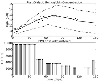
Fig. 1. The upper panel shows the model output for the initial parameter value sets that were used and model output for the ’optimal’ parameter. Stars denote measured data. The lower panel shows the administered EPO doses.
algorithm. In fact, in [15] a counterexample is presented for a family of strictly convex functions in two dimensions. Despite, these unsatisfying theoretical results, Nelder-Mead seems to do quite well in practice and is a widely used optimization method. One just has to be careful to make sure that the algorithm does not get stuck at a non-optimal point. Hence, you may want to restart the algorithm with slightly modified parameter values to alleviate this problem.
IV. NUMERICALRESULTS
The numerical approximation scheme described in Sec-tion III was implemented in Python, see [16]. Further, we use the Nelder-Mead simplex method implemented in the SciPy package (see [17]) for Python to minimize the cost-functional given in equation (2).
The model is adapted to an individual CKD patient by adjusting the following parameters: the total blood volume, number of stem cells committing to the erythroid lineage per day, the bone marrow response to EPO, half-life of the administered EPO compound, RBC lifespan and endogenous EPO level. Some of those parameters are estimated using empirical formulae using information on gender, height and weight and the remaining parameters are determined using the method described in Section III. For further details see Appendix. The question how well a certain set of parameters is identifiable for a given set of data, i.e. for a certain model output, is not a trivial one. Some sets of parameters are better identifiable than others; and certain parameters might be almost impossible to identify using a specific set of data. The problem is, the data may not contain a lot of information on a specific parameter and some parameters are simply not identifiable simultaneously1 For a good overview on sensitivity analysis and a discussion for different approaches to subset selection see e.g. [18]–[20]. Hence, for the sake of simplicity and to avoid to select a subset of parameters which
1A trivial example isy˙= (p
1/p2)y.Whereask=p1/p2is obviously
identifiable (growth/decay-rate of an exponential process) we have no means to identify the parametersp1andp2 simultaneously, due to the ambiguity
initSet1 initSet2
N p1 p2 p1 p2
8 71.3589 15.0967 71.3599 15.0956 10 63.1753 20.997 63.1755 20.9969 14 63.0866 21.0543 63.0867 21.0544 20 63.0237 21.1054 63.0238 21.1054
30 63.0314 21.0979 63.0313 21.0979 40 63.0263 21.0995 63.0263 21.0994 50 63.0112 21.1092 63.0112 21.1092 60 63.0532 21.081 63.0531 21.081
TABLE I
PARAMETER ESTIMATES OBTAINED USING TWO SETS OF STARTING VALUES FOR THE OPTIMIZATION ALGORITHM.
is difficult to estimate, we focus in this paper on identifying two parameters simultaneously, using the Hgb measurements from the Crit-Line device: RBC lifespan and endogenous EPO level.
The ’optimal’ parameters for the RBC lifespan p1 and
endogenous EPO level p2 were estimated to be: p1 =
63.05 andp2 = 21.08. Thus, our optimal parameter set is optSet= (63.05,21.08). We define two sets of initial values:
initSet1 = (56,18.75)andinitSet2 = (70,23.125), which corresponds to a perturbation of the parameters of about
±10%. Further, we start parameter identification runs for both sets of initial parameters for an increasing approxi-mation dimension N. Ideally, the parameter identifications would give the same results, regardless of the set of initial values which is used. Moreover, one would hope that with increasingNthe estimated parameter values would express a convergent behavior. In Figure 1 we present the model output for both initial parameter setsinitSet1andinitSet2, as well as the model output for the optimal parameter set and the data measured. All three model simulations were determined using an approximation dimension of N = 60.
In Table I the results of the parameter identification runs forN = 8,10,14,20,30,40,50,60for the initial parameter sets initSet1 = (56,18.75) and initSet2 = (70,23.125)
are shown. It can be observed that the estimated parameters for initSet1 and initSet2 are close to each other for all
N. These findings confirm that the estimated parameter sets indeed are minimizers of the cost-functionalJ(p1, p2)given
in equation 2 and that the Nelder-Mead simplex algorithm does not get stuck in a non-optimal point. Further, the fact that a perturbation of the optimal parameter values of
±10% provides the same estimates when minimizing the cost-functionalJ(p1, p2)and is – for at leastN≥10– very
close to the original value, implies that the parameter subset chosen is (locally) well identifiable. Moreover, from Table I one can see that, the parameter estimates for increasing approximation dimensions N show a convergent behavior. Whereas for N = 8 the estimates for p1 and p2 differ
distinctly from optSet = (63.05,21.08), for N = 10 the estimated parameter set is already very close, (p1, p2) =
(63.1753,20.997). A further increase of the approximation dimension, results only in minor changes of the estimated parameter values.
In Figure 2 we compare the model outputs for N = 10
(solid line) andN = 60(dashed line) and the corresponding
0
30
60
90
120
150
9.5
10.0
10.5
11.0
11.5
12.0
12.5
13.0
13.5
Hgb [g/dl]
Post-Dialytic Hemoglobin Concentration
Fig. 2. Model output for N=10 (solid line) and N=60 (dashed line). Stars denote measured data.
parameter estimations, i.e.(p1, p2) = (63.1753,20.997)and
(p1, p2) = (63.0532,21.081), respectively. The difference
between the two simulations is barely recognizable. Looking closely at the graphs one can observe a very small discrep-ancy around day 50 – 90.
V. CONCLUSION
Our findings suggest that the parameter subset – RBC lifespan and endogenous EPO level – is (locally) well identifiable using frequent measurements (3 times per week) for hemoglobin concentration. Further, the solutions of the minimization process of the cost-functional for different approximation dimensions seem to converge. Moreover, it seems that an approximation dimension ofN = 10suffices to get a sufficient accurate estimate for the parameter subset and that the numerical solution does not express (distinct) oscillatory behavior.
APPENDIX
The erythropoiesis model presented in [5] is adapted to an individual CKD patient by adjusting the following parameters: the total blood volume T BV, number of stem cells S0 committing to the erythroid lineage per day, the
bone marrow response to EPO2, half-life cex
deg of the drug EPO , RBC lifespanµm
max and endogenous EPO levelEend.
Note, the notation of the parameters used here is conform with the notation used in [5]. For a list of the values for the adapted parameters see Table II. TBV and stem cells committing to the erythroid lineage were estimated using an empirical formula (see [12]). The remaining parameters were estimated using the parameter identification scheme presented in Section II. Further, we have to mention that in a healthy person the endogenous EPO levelEendis modeled using a compartment equation considering the amount of EPO released by the kidneys (varies over time) and the degradation rate (constant over time). In general, the kidneys react to a change in red blood cell mass by adapting the
2We adapt the slope of the sigmoidal functions which describe how
the death rate of the CFU-E cellsk1 and the maturation velocity of the
Parameter Meaning Value Unit
TBV total blood volume 4000 ml
S0 rate at which cells are
committing to the erythroid lineage
6.64·106
1/d
k1 constant for the sigmoid
apoptosis rate for CFU-E cells
0.006788 ml/mU
k2 constant for the sigmoid
maturation velocity for reticulocytes
0.18888 ml/mU
cex
deg degradation rate of
administered EPO
4.4/24 1/d
µmax maximal life span for
erythrocytes
63.05 d
Eend endogenous EPO level 21.08 mU/ml
TABLE II
VALUES OF THE ADJUSTED PARAMETERS FOR THE DIALYSIS PATIENT SHOWN INFIGURE1AND2.
amount of EPO segregated. In the special setting of CKD it is reasonable to assume that there is a low constant baseline production of EPO by the kidneys. Thus, we adjust for those patients the (constant) endogenous EPO level instead of the change in productivity of the kidneys.
REFERENCES
[1] A. Besarab, W. Bolton, J. Browne, J. Egrie, A. Nissenson, D. Okamoto, S. Schwab, and D. Goodkin, “The effects of normal as compared with low hematocrit values in patients with cardiac disease who are receiving hemodialysis and epoetin,”The New England Journal of Medicine, vol. 339, pp. 584–590, 1998.
[2] A. Go, G. Chertow, D. Fan, C. McCulloch, and C. Hsu, “Chronic kidney disease and the risks of death, cardiovascular events, and hospitalization,”The New England Journal of Medicine, vol. 351, pp. 1296–1305, 2004.
[3] G. Strippoli, J. Craig, C. Manno, and F. Schena, “Hemoglobin targets for the anemia of chronic kidney disease: A meta-analysis of random-ized, controlled trials,”Journal of American Society of Nephrology, vol. 15, pp. 3154–3165, 2004.
[4] M. Lichtman, E. Beutler, T. Kipps, U. Seligsohn, K. Kaushansky, and J. Prchal, Eds.,Williams Hematology, 7th ed. McGraw-Hill, 2005. [5] D. Fuertinger, F. Kappel, S. Thijssen, N. Levin, and P. Kotanko, “A
model of erythropoiesis in adults with sufficient iron availability,”
Journal of Mathematical Biology, vol. 66, no. 6, pp. 1209–1240, 2013, DOI: 10.1007/s00285-012-0530-0.
[6] D. Fuertinger, “A model for erythropoiesis,” Ph.D. dissertation, Uni-versity of Graz, Austria, 2012.
[7] A. Collins, R. Brenner, J. Ofman, E. Chi, N. Stuccio-White, M. Kr-ishnan, C. Solid, N. Ofsthun, and J. Lazarus, “Epoetin alfa use in patients with ESRD: an analysis of recent US prescribing patterns and hemoglobin outcomes.”American Journal of Kidney Diseases, vol. 46, pp. 481–488, 2005.
[8] S. Fishbane and J. Berns, “Hemoglobin cycling in hemodialysis patients treated with recombinant human erythropoietin,” Kidney In-ternational, vol. 68, pp. 1337–1343, 2005.
[9] K.-J. Engel and R. Nagel, One Parameter-Semigroups for Linear Evolution Equations. Springer, 2000.
[10] K. Ito and F. Kappel,Evolution Equations and Approximations. World Scientific, 2002.
[11] F. Kappel and K. Zhang, “Approximation of linear age-structured pop-ulation model using Legendre polynomials,”Journal of Mathematical Analysis and Applications, vol. 180, pp. 518–549, 1993.
[12] S. Nadler, J. Hidalgo, and T. Bloch, “Prediction of blood volume in normal human adults,”Surgery, vol. 51, pp. 224–232, 1962. [13] J. Nelder and R. Mead, “A simplex method for function minimization,”
Computer Journal, vol. 7, pp. 308–313, 1965.
[14] J. Nocedal and S. Wright, Numerical Approximation, 2nd ed., ser. Operations Research and Financial Engineering. Springer, 2006. [15] K. McKinnon, “Convergence of the Nelder-Mead simplex method to a
nonstationary point,”SIAM Journal on Optimization, vol. 9, pp. 431– 441, 1996.
[16] G. van Rossum and F. L. Drake, Eds.,Python Reference Manual.
http://docs.python.org/ref/ref.html: Python Software Foundation, 2012.
[17] E. Jones, T. Oliphant, P. Petersonet al., “SciPy: Open source scientific tools for Python,” http://www.scipy.org/, 2001–.
[18] H. Miao, X. Xia, A. S. Perelson, and H. Wu, “On identifiability of nonlinear ODE models and applications in viral dynamics,”SIAM Rev., vol. 53, pp. 3 – 39, 2011.
[19] E. Walter and L. Pronzato, “Qualitative and quantitative experiment de-sign for phenomenological models — A survey,”Automatica, vol. 26, no. 2, pp. 195 – 213, 1990.