Maintaining homeostasis by decision-making.

(1)

Maintaining Homeostasis by

Decision-Making

Christoph W. Korn1*, Dominik R. Bach1,2

1Department of Psychiatry, Psychotherapy, and Psychosomatics, University of Zurich, Zurich, Switzerland,

2Wellcome Trust Centre for Neuroimaging, University College London, London, United Kingdom

Abstract

Living organisms need to maintain energetic homeostasis. For many species, this implies taking actions with delayed consequences. For example, humans may have to decide be-tween foraging for high-calorie but hard-to-get, and low-calorie but easy-to-get food, under threat of starvation. Homeostatic principles prescribe decisions that maximize the probabili-ty of sustaining appropriate energy levels across the entire foraging trajectory. Here, predic-tions from biological principles contrast with predicpredic-tions from economic decision-making models based on maximizing the utility of the endpoint outcome of a choice. To empirically arbitrate between the predictions of biological and economic models for individual human decision-making, we devised a virtual foraging task in which players chose repeatedly be-tween two foraging environments, lost energy by the passage of time, and gained energy probabilistically according to the statistics of the environment they chose. Reaching zero energy was framed as starvation. We used the mathematics of random walks to derive end-point outcome distributions of the choices. This also furnished equivalent lotteries, pre-sented in a purely economic, casino-like frame, in which starvation corresponded to winning nothing. Bayesian model comparison showed that—in both the foraging and the casino frames—participants’choices depended jointly on the probability of starvation and the ex-pected endpoint value of the outcome, but could not be explained by economic models based on combinations of statistical moments or on rank-dependent utility. This implies that under precisely defined constraints biological principles are better suited to explain human decision-making than economic models based on endpoint utility maximization.

Author Summary

Common decision-making models arise from firm axiomatic foundations but do not ac-count for a variety of empirically observed choice patterns such as risk attitudes in the face of high-impact events. Here, we argue that one reason for this mismatch between theory and data lies in the neglect of basic biological principles such as metabolic homeostasis. We use Bayesian model comparison to show that models based on homeostatic

consider-ations explain human decisions better than classic economic models—both in a novel

vir-tual foraging task and in standard economic gambles. Specifically, we show that in line

OPEN ACCESS

Citation:Korn CW, Bach DR (2015) Maintaining Homeostasis by Decision-Making. PLoS Comput Biol 11(5): e1004301. doi:10.1371/journal.pcbi.1004301

Editor:Jill X O'Reilly, Oxford University, UNITED KINGDOM

Received:January 20, 2015

Accepted:April 27, 2015

Published:May 29, 2015

Creative Commons Attribution License, which permits unrestricted use, distribution, and reproduction in any medium, provided the original author and source are credited.

Data Availability Statement:All relevant data are within the paper and its Supporting Information files.

S1 Datasetcontains the behavioral data of all subjects.

Funding:This work was funded by the University of Zurich. The Wellcome Trust Centre for Neuroimaging is supported by core funding from the Wellcome Trust [091593/Z/10/Z]. The funders had no role in study design, data collection and analysis, decision to publish, or preparation of the manuscript.

(2)

with the principle of homeostasis human choice minimizes the probability of reaching a lower bound. Our results highlight that predictions from biological principles provide sim-ple, testable, and ecologically rational explanations for apparent biases in decision-making.

Introduction

Homeostasis is paramount to all living organisms [1]. Put simply, organisms have to maintain

their internal milieu within certain boundaries to avoid dying. This homeostatic principle

re-verberates on the levels of molecular interactions [2], hormonal feedback loops [3,4], neural

circuits [5], and psychophysiological processes [6]. Beyond the need for immediate regulation,

many species face complex decisions with delayed and probabilistic consequences for long-term metabolic homeostasis. Here, we hypothesize that homeostatic requirements guide forag-ing decisions in humans. For example, huntforag-ing deer provides a large energy gain with low probability of obtaining it, while collecting berries provides a small energy gain with high prob-ability. In order to minimize the probability of starvation, human agents should integrate the statistics of the available options with their current energy levels and with their time horizon.

Classical views of homeostasis [1–7] are often illustrated with a thermostat that senses the

difference between a temperature set point and the current temperature. This deviation value elicits a change in heating levels. The thermostat is thus supposed to retrospectively compen-sate deviations that have already manifested themselves. In contrast, we propose that decision-makers can anticipate possible deviations and proactively minimize the probability of reaching a prohibitive boundary such as starvation. This extends established notions of homeostasis in

(psycho)physiology [1–7] and is concordant with recent theoretical accounts of homeostasis as

a principle explaining decision-making in healthy and psychiatric populations [8–10].

When applied to individual decision-making, predictions from this model are in

contradis-tinction to economic models which firmly rest upon axiomatic foundations [11] and elegantly

explain many types of monetary decisions [12]. These models posit that decision-makers base

their choices on the utility assigned to the endpoint outcome of a choice irrespective of the tra-jectory to this endpoint [12–14].

In risk-return models and their variants [13,15], the endpoint utility is computed via

statisti-cal moments of an outcome distribution, usually expected value, variance, and in some models also skewness. A considerable literature has generalized risk-return models to include

subjec-tive transformations of statistical moments [15,16]. In behavioral economics, variants of

risk-return models have been widely used to describe how humans choose between monetary

gam-bles [17–19], how they assess real-life events [16], and how animals decide on primary

rein-forcers [20,21]. Expected utility theory and its derivations constitute another class of models in

which values of possible outcomes are transformed into an internal utility measure by a

deci-sion-maker's individual utility function [12,15,22]. Rank-dependent utility models additionally

supplement a non-linear weighting of the option’s outcome probabilities [23,24]. Similar to

risk-return models, rank-dependent utility models have been used extensively to describe em-pirical data both from the lab and the field [15,23,24].

Empirically observed deviations from predictions of these microeconomic models are often framed as irrational biases, and additional parameters are included to absorb such biases, but often without making principled assumptions on why these influences should arise in the first

place [25]. Here, we furnish a principled biological reason for deviations from economic

(3)

the internal milieu. We sought to show that even in a safe laboratory environment, a decision-making model based on homeostatic principles could explain foraging decisions better than economic models. Further, we hypothesized that homeostatic considerations would also guide human decision-making for simply structured lotteries without any reference to foraging, as

often employed in behavioral economics [12–14,26].

To test these hypotheses, we developed a virtual foraging task. In each trial, human

partici-pants chose between two“foraging environments”with different possible“energy”gains and

associated probabilities, in which they would forage for up to three consecutive“days”(see

Fig 1Afor illustration). At the time of choice, an energy bar depicted participants’current in-ternal state. Participants were instructed that on each foraging day, they would lose one energy point, and gain energy according to the statistics of the chosen environment. Successive days in the task required the integration of risks from multiple foraging attempts. For each trial, partic-ipants made a single decision between the two foraging environments for the indicated number

of days. Losing all energy points on any day in a given foraging period was framed as“

starva-tion”but was not explicitly punished. Each trial was independent. We did not give feedback on

choice outcomes of their choices or intermediate states of the foraging sequence. At the end of the experiment, participants were rewarded for the endpoint foraging outcome of two random-ly selected trials. Starvation meant that participants did not win anything from the trial. We hy-pothesized that participants would compute the probability of starvation for the foraging environments and base their decisions on this metric.

We used the mathematics of random walks to analytically derive the distributions of the endpoint outcomes of the foraging period, and of the probabilities of starvation during foraging (seeFig 1Cfor a graphical illustration,Fig 1Dfor an example of the variables derived by this

procedure,Table 1for a summary of the gambles, andMethodsandS1 Textfor mathematical

details). Because participants were only rewarded for endpoint outcomes, homeostatic princi-ples are irrelevant for maximizing utility, yet our task was suggestive of using them. Hence, we tested whether such principles also influence decisions when they are not invoked by the task frame. We presented participants with purely economic gambles, framed as wheel-spinning

ca-sino lotteries without any reference to foraging (seeFig 1B). These lotteries had identical

end-point outcomes as the foraging environments. The probability of starvation in the foraging frame corresponded to the probability of winning nothing in the casino frame. As in the forag-ing frame, participants did not receive feedback on the outcomes of their choices. In addition to the instruction, the two frames differed in the fact that options in the foraging frame were presented as gamble sequences when the number of days was greater than one, whereas options in the casino frame were always single-step gambles. To avoid foraging instructions influencing behavior in the casino frame, the casino frame preceded the foraging frame for all participants.

Results

Overall comparison of model families across both frames

We first asked whether models based on homeostatic principles explain choice better than

standard economic models—both in a foraging and in a casino frame. We combined choices

from both frames and compared three families of formal decision-making models. The first two model families included variations of two types of economic models while the third family

comprised models based on homeostatic considerations (seeMethodsandTable 2for details).

In line with our hypothesis that participants’decisions should take into account the

proba-bility of starvation (pstarve), the homeostatic model family provided the significantly best fit.

(4)

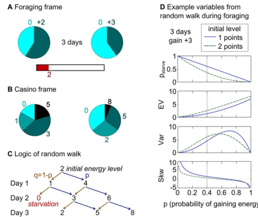
Fig 1. Virtual foraging task and derivation of the gambles. (A)Foraging frame: In each trial, participants saw an energy bar depicting their initial energy points. Participants had to decide between two foraging options, which were depicted as pie charts with two sectors: the light blue sectors corresponded to unsuccessful foraging (i.e., to a gain of zero points), the dark blue sectors corresponded to successful foraging (i.e., to a gain of the number of points written above the sectors). In each trial, participants made a single decision and the chosen foraging option was played out for the specified number of“days.”For each day, the probabilistic outcome of the chosen foraging option was determined and the respective gains were added to the energy bar. A sure cost of one point was deducted on each day to mirror energy consumption. If at any day the energy bar reached zero, the participant died from starvation in that trial. We denote this probability as pstarve. The choice in the foraging frame was therefore between two gamble sequences, where

the number of days indicated the number of gambles in each sequence. Participants did not see the outcomes of their choices but were presented with examples in the written instructions.(B)Casino frame: Numerically identical gambles as in the foraging frame were presented as pie charts similar to wheel-spinning gambles in a casino. The size of each sector denoted the probability of winning the amount written next to it. In the casino frame, pstarvewas directly visible as the size of the sector for an outcome of zero. The choice in

the casino frame was thus between two single-step gambles.(C)Illustration of the logic behind the mathematics of random walks, which we used to derive the gambles (seeS1 Textfor mathematical details). The tree-like illustration depicts the random walk used to calculate the variables of the right gambles in A and B. The random walk starts at position“2”which corresponds to the initial number of energy points. In each step (“day”) the agent walks to the“right”with probability p (corresponding to successful foraging; dark blue sector of pie chart in A) or to the“left”with probability 1-p (corresponding to unsuccessful foraging; light blue sector of pie chart in A). The step size to the“left”corresponds to the sure cost and is always one. The step size to the right depends on the amount of energy points to gain (here there are +3 points and thus the step size is +2 because the sure cost has to be subtracted). Zero is an absorbing boundary and thus no arrows start from zero. The possible outcomes are directly visible in the casino frame (here 0, 2, 5, and 8 points). To determine the probability of a specific outcome one has to follow all possible paths along the branches of the tree leading to that outcome and sum over their probabilities. The probabilities of a specific“path along the branches”are determined by multiplying the probabilities of all arrows on that path. In the current example, the probability of an outcome of zero (i.e., pstarve) is q2and the probability of an outcome of 2 is 2pq2.(D)

Distribution of the variables for the random walk shown in C across all values of p (i.e., the probability of successful foraging or of going right in the random walk). In the example of the right gamble shown in A and B, p was chosen at 40% and the intersection of the black vertical lines with the green lines give the variables for the current example (i.e., for an initial energy level of 2 energy points).

(5)

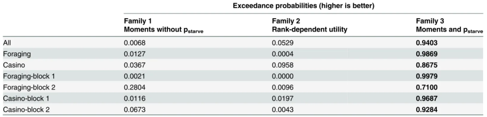
the population was 0.9403 (Table 3). Under the assumption that all participants use the same model (fixed-effects analysis), the winning model belonged to the homeostatic family (see

Fig 2AandTable 2for log-group Bayes factors based on the Bayesian information criterion

(BIC) relative to the simplest model; seeS2 TextSection 7 andS1 TableandS2 Tablefor results

based on the Akaike information criterion, AIC; seeS3 Tablefor the fits of the different models

for each individual participant). Thus, the overall comparison of model families confirmed our hypothesis that starvation probability and thus homeostatic principles provided explanatory

power in explaining participants’behavior, over and above economic variables, and although

irrelevant for utility maximization in the laboratory.

Table 1. Variables of the 480 binary gambles used in the task.

Variable Range Mean SD

Initial state (x0) 1–2 -

-Days (n) 1–3 -

-Gains (g) 2–6 -

-Probabilities of individual options 0.008–0.9 -

-EV 1.47–5.53 3.18 1.16

Var 0.75–27.59 8.45 6.61

Skw -2.67–2.00 0.00 0.76

pstarve 0.06–0.77 0.35 0.16

The means and SD of EV, Var, Skw, and pstarvewere calculated over both options of the binary gambles.

SD, standard deviation; EV, expected value; Var, variance; Skw, skewness; pstarvestarvation probability doi:10.1371/journal.pcbi.1004301.t001

Table 2. Model family comparison: Relative log-group Bayes factors.

Relative log-group Bayes factors (smaller is better)

Family 1 Family 2 Family 3

Moments without pstarve Rank-dependent utility Moments and pstarve

Model Model Model Model Model Model Model Model Model

1 2 3 4 5 6 7 8 9

EV EV EV EV Prelec-I Prelec-II EV EV EV

Var Skw Var pstarve Var Var

Skw pstarve Skw

pstarve

All 0 -1333 -1984 -2032 -2154 -2148 -2191 -2167 -2126

Foraging 0 -884 -1390 -1437 -1466 -1390 -1511 -1532 -1569

Casino 0 -709 -945 -967 -1040 -1023 -1062 -1044 -970

Foraging-block 1 0 -472 -683 -696 -734 -679 -781 -751 -741

Foraging-block 2 0 -412 -661 -729 -725 -689 -751 -737 -773

Casino-block 1 0 -363 -451 -456 -488 -465 -518 -487 -439

Casino-block 2 0 -342 -519 -507 -525 -463 -565 -537 -487

For aﬁxed-effects analysis, log-group Bayes factors based on BIC were calculated relative to the simplest model (Model 1). Smaller log-group Bayes factors indicate more evidence for the respective model versus the baseline model. The log-group Bayes factors of the winning models according toﬁ xed-effects analyses are written in bold font. The models included free parameters for the respective variables listed. BIC, Bayesian information criterion; EV, expected value; Var, variance; Skw, skewness; pstarvestarvation probability

(6)

Frame-specific comparison of model families

Next, we separately analyzed choices in the foraging frame and in the purely monetary context of the casino frame, by comparing the three model families within each frame. The same

over-all pattern emerged. The homeostatic family, in which models included pstarve, had the highest

exceedance probabilities in both frames independently (foraging: 0.9869; casino: 0.8675;

Table 3). Also, the models winning in fixed-effects analyses belonged to the homeostatic family (seeTable 2for log-group Bayes factors based on BIC). Further, when we fitted the models

Table 3. Model family comparison: Exceedance probabilities.

Exceedance probabilities (higher is better)

Family 1 Family 2 Family 3

Moments without pstarve Rank-dependent utility Moments and pstarve

All 0.0068 0.0529 0.9403

Foraging 0.0127 0.0004 0.9869

Casino 0.0367 0.0958 0.8675

Foraging-block 1 0.0021 0.0000 0.9979

Foraging-block 2 0.2804 0.0096 0.7100

Casino-block 1 0.0116 0.0197 0.9687

Casino-block 2 0.0673 0.0043 0.9284

The highest exceedance probabilities according to random-effects analyses are written in bold font. BIC, Bayesian information criterion; pstarve

starvation probability

doi:10.1371/journal.pcbi.1004301.t003

Fig 2. Results of model comparison. (A)Log-group Bayes factors (smaller is better) relative to the simplest models (Model 1) based on BIC for the nine models tested (left part) and histogram of best-performing models per participant (right part). The models belonged to three families. In the first family, models were based on various combinations of weighting parameters for the first three statistical moments (i.e., EV, Var, and Skw). The second family comprised two rank-dependent utility models in which probabilities were weighted according to non-linear weighting functions (Prelec-I and Prelec-II). In the third family, models were based on the homeostatic principle of minimizing pstarvein addition to combinations of weighting parameters for the statistical

moments. Across both frames, the third model family provided the best fit to the data. For ease of reference, the first two models are not depicted because their log-group Bayes factors were far off relative to the other models. The histogram shows that in 11 of 22 participants the best performing model belonged to the third model family. Note that the fixed-effects analyses do not account for possible outliers, while random-effects analyses do. Smaller log-group Bayes factors indicate more evidence for the respective model versus the baseline model. See alsoTable 2.(B)Parameter estimates from an adaptation of the overall winning model for foraging-pstarve(ξforaging) and casino-pstarve(ξcasino) for individual participants. As expected from the notion that participants should

minimize pstarve, most parameter estimates were negative (i.e., in the lower left quadrant). Additionally, for most participants foraging-pstarvewas more

(7)

separately for the first and second blocks of the foraging and casino frames, the same pattern emerged in all analyses. The homeostatic family had the highest exceedance probabilities and

models belonging to this family won the fixed effects analyses (see Tables2and3; seeS2 Text

Section 7,S1 TableandS2 Tablefor results based on AIC).

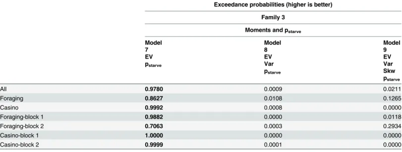
Comparison within winning model family

Within the winning model family, we analyzed which specific model best explained choices. In a random-effects analysis, the exceedance probability of the simplest homeostatic model was

0.9786 across both frames (Table 4). Similar results emerged when fitting the models separately

within the two frames or separately to the first and second blocks (Table 4; seeS2 TextSection

7 andS4 Tablefor results based on AIC; seeS1 Figfor binned choice data). In this winning

model, the decision variable was a linear combination of difference in starvation probability

(pstarve) weighed by a parameterξ, and difference in expected value (EV). This decision variable

was transformed into a decision probability by a sigmoid function with another parameter,β.

Comparison of parameters in an adapted version of the winning model

The previous analyses showed that participants consistently used models based on homeostatic

principles in both frames. This leaves open the question how participants used pstarveand

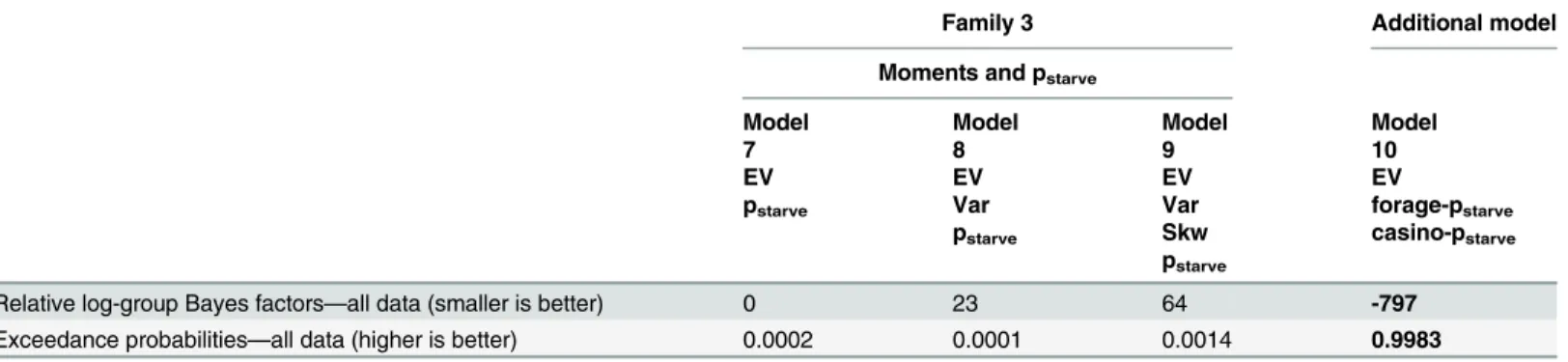
whether this differed between the two frames. Hence, we added frame-specific free parameters to the winning model and then tested the parameter estimates across participants.

Specifically, we adapted the winning model (Model 7), which included two free parameters:

a parameterβfor the decision noise and a parameterξto quantify the impact of pstarveon

par-ticipants’decision. This parameterξwas replaced by two frame-specific weighting parameters

(ξforagingandξcasino). We added this model (Model 10) to the initial set of three models in the

Table 4. Comparison within the winning model family: Exceedance probabilities.

Exceedance probabilities (higher is better)

Family 3

Moments and pstarve

Model Model Model

7 8 9

EV EV EV

pstarve Var Var

pstarve Skw

pstarve

All 0.9780 0.0009 0.0211

Foraging 0.8627 0.0108 0.1265

Casino 0.9992 0.0008 0.0000

Foraging-block 1 0.9882 0.0000 0.0118

Foraging-block 2 0.7063 0.0003 0.2934

Casino-block 1 1.0000 0.0000 0.0000

Casino-block 2 0.9999 0.0001 0.0000

The highest exceedance probabilities according to random-effects analyses are written in bold font. BIC, Bayesian information criterion; EV, expected value; Var, variance; Skw, skewness; pstarvestarvation probability

(8)

third family. Despite being penalized for the additional free parameter, it explained choices bet-ter than the other three models considered. Its exceedance probability was 0.9983 in a random-effects analysis and it had the smallest log-group Bayes factor in a fixed-random-effects analysis (Table 5; seeS2 TextSection 7 andS5 Tablefor results based on AIC). This indicates that

par-ticipants weighted pstarvedifferently in the two frames.

Crucially, our prediction that participants’choices minimize pstarverequires that weighting

parameters of pstarvebe negative. Indeed, the parameters for the frame-specific parameters

ξfora-gingandξcasinowere significantly smaller than zero across participants (sign test on parameters

in the overall winning model:ξforaging: p<.001; andξcasino: p<.005;Fig 2B). That is, participants

chose the gambles with the smaller pstarveand thus minimized pstarve. Additionally, across

par-ticipantsξforagingwas smaller thanξcasino(sign test comparingξforagingandξcasino: p<.05).

In line with the above analyses, supporting analyses showed that pstarveplayed a greater role

than EV in the foraging frame, while in the casino frame EV played a greater role than pstarve,

for explaining choices (seeS2 TextSection 1 andS6 Tablefor details). Additionally, we devised

a supplemental model to test whether the different number of foraging days led to a different

weighting of pstarvebut did not find evidence supporting this idea (S2 TextSection 2 andS7

Table). We also found no evidence supporting the hypothesis that different combinations of

energy levels and foraging days lead to differential weighting of pstarve(S2 TextSection 4).

Sup-plementary analysis showed that participants did not erroneously include values below zero in

their estimation of the outcome distributions in the foraging frame (S2 TextSection 5 andS8

Table). In an exploratory analysis, we also found no evidence for a relationship of the model

parameters to participants’meta-cognitive risk assessments on the domain-specific

risk-atti-tude scale (S2 TextSection 8).

Taken together, participants consistently minimized pstarvein both frames and did so more

in the foraging than in the casino frame.

Analyses of reaction times

Can reaction times (RTs) as a tentative measure of choice difficulty give us additional evidence for the relevance of homeostatic principles? Since our model comparison showed that EV and

Table 5. Comparison of an additional model including frame-specific parameters: Relative log-group Bayes factors and exceedance probabilities.

Family 3 Additional model

Moments and pstarve

Model Model Model Model

7 8 9 10

EV EV EV EV

pstarve Var Var forage-pstarve

pstarve Skw casino-pstarve pstarve

Relative log-group Bayes factors—all data (smaller is better) 0 23 64 -797

Exceedance probabilities—all data (higher is better) 0.0002 0.0001 0.0014 0.9983

Log-group Bayes factors based on BIC were calculated relative to the simplest model (Model 7). Smaller log-group Bayes factors indicate more evidence for the respective model versus the baseline model. The log-group Bayes factor of the winning model according toﬁxed-effects analysis and the highest exceedance probability according to random-effects analysis are written in bold font. BIC, Bayesian information criterion; EV, expected value; Var, variance; Skw, skewness; pstarvestarvation probability

(9)

pstarveexplained participants’choices, we tested whether EV and pstarvealso related to RTs.

That is, we tested whether RTs were faster for larger absolute differences between the two

op-tions in EV and pstarve. This was indeed the case as shown by a linear mixed effects model on

log-transformed RTs (EV: t = -4. 98, p<.001; pstarve: t = -2.62, p<.05; significance levels were

determined by log-likelihood tests, comparing the full model to a model without the respective

factor). The interaction of EV and pstarvewas significant and related to slower RTs (t = 3.52,

p<.005). SeeS1 Figfor binned RT data. In sum, a combination of EV and pstarvewas related to

choice difficulty as indexed by RTs, which corroborates that homeostatic principles guided participants’choices.

Discussion

This study addressed whether homeostatic principles explain human decision-making over and above previously described economic models based on endpoint utility maximization. We found that human decisions minimized the probability of reaching a lower homeostatic bound on the trajectory to their endpoint outcomes, despite the fact that our tasks did not entail any explicit negative consequences of reaching this boundary. This was evident both in a virtual foraging task, in which the possibility of starvation was a salient task feature, and in a casino-like frame, in which only the endpoint outcomes of the gambles and their associated probabili-ties were explicitly stated. Our fine grained model comparison provided evidence that the deci-sion variable in the most parsimonious model was based on a linear combination of the probability of starvation and endpoint expected value (EV), outperforming standard economic models.

The maximization of endpoint EV lies at the core of many variants of axiomatically derived microeconomic models. However, neither variants of risk-return models nor variants of ex-pected utility theory predict that decisions minimize the probability of reaching a lower ho-meostatic bound before that endpoint is realized. The winning model family included the probability of zero outcomes although we did incentivize participants to avoid them, and al-though zero outcomes are already incorporated into the calculation of statistical moments and utilities. For a description of behavior, we could have used a very specific shape of the utility function which assigns a high negative utility to the zero outcome and positive utility to neigh-boring positive outcome, in contrast to typical utility functions in the economic literature. However, such a model would neither be more parsimonious than ours, nor offer any addition-al explanatory power.

We note that in the best fitting model, the decision variable was a linear mixture of outcome variables and thus it did not differ from previous risk-return models in its mathematical struc-ture. Crucially, minimization of the probability of a zero outcome provided more explanatory power than risk-attitudes based on variance or skewness. Thus, our results are in line with previous accounts calling for more fine-grained and possibly context-dependent metrics

within the framework of risk-return models [19,27]. Additionally, our model only makes

meaningful predictions when the probability of threats to homeostasis is nonzero and thus our approach has the desirable feature that the scope of the model is under precisely defined constraints.

We provide evidence that the homeostatic principle of avoiding a lower boundary on energy levels pervades human decision-making. Classical descriptions often relate homeostatic

pro-cesses to the actions of a thermostat [6,7]. The thermostat example best fits to physiological

variables with a narrow homeostatic range, for which this range can be approximated by a set

point (e.g., blood pH) [7]. For other variables the homeostatic range is larger. In the case of

(10)

homeostatic counter-measures occur at the boundaries of this range [7]. For simplicity, we as-sumed starvation to be a hard boundary but the same principle would apply for soft bound-aries. More importantly, our results extend the notion exemplified by the thermostat analogy. In line with recent theoretical views on homeostasis in healthy and psychiatric populations

[8,10], we conjectured that human decision-makers can estimate the probability of future

dis-ruptions to homeostasis. Thus, in contrast to a thermostat that can only react to homeostatic

threats once they have occurred, human—and possibly many animal—decision-makers can

proactively avoid threats to homeostasis.

The same model performed best in both the foraging frame and in the casino frame. We highlight this similarity between the two frames because it shows that the homeostatic principle of minimizing the probability of a zero outcome is at play even when participants are not primed by the task description to do so. Furthermore, the same model explains behavior in gamble sequences and in single-step gambles. In the casino frame, the probability of starvation was directly depicted by the size of the sector in the pie chart that indicated the probability for the zero outcome. Strikingly, in the foraging frame participants integrated the probabilities of gaining energy over the indicated number of days to compute the probability of starvation. Par-ticipants could not learn the outcome distributions through experience because we did not pro-vide them with feedback. Thus, decisions in the foraging frame were not dependent on

participants having directly experienced sequences in the virtual foraging environments. Risky decision-making differs depending on whether outcome distributions are described or learned

from experience [22,28]. For example, rare events tend to exert less impact in decisions based

on experience. Our results suggest that such an underweighting might not occur for the proba-bility of starvation [28].

Within the winning model, more fine grained analyses revealed differences between the two frames in the best-fitting parameter estimates. The probability of starvation in the foraging

frame had a greater impact on participants’decisions than the corresponding probability of

re-ceiving nothing in the casino frame—an effect unrelated to the sequential versus single-step

presentation of the gambles (seeS2 TextSection 3). This was the case even though participants

had to compute the probability of starvation in the foraging frame by combining information about internal state, foraging options, and time horizon. Approximating starvation probabili-ties may become more difficult and thus imprecise as the number of steps increases. In the cur-rent study, participants were able to approximate the probability of starvation with sufficient accuracy for at least three steps, as their decisions were based on this metric.

The structure of our tasks complies with the requirements of economic paradigms such as

complete knowledge and incentive-compatibility [12]. Thus, specific task characteristics are

unlikely to explain why our homeostatic model outperformed standard economic models, based on statistical moments [15,17,18] or non-linear probability weighting [23,24]. Instead, we reason that the biological constraints relevant in ecological contexts such as hunting or

farming exert a prevailing impact on human decisions in the laboratory—even if apparently

ir-relevant to the task at hand. A similar rationale has recently been advocated in discussions of

whether animal [29,30] and human [31–34] decision-making deviates from normative models.

According to probabilistic accounts of brain function, the brain uses prior probabilities to per-form probabilistic inferences [8,14,35,36]. These prior probabilities are tuned—by evolution

and/or experience—to the natural statistics of real world environments [30,31]. Consequently,

human and non-human decision-makers may behave rationally according to their beliefs but they appear irrational because those beliefs are not warranted in deliberately simplified

labora-tory tasks or in some other contexts [30,37]. Overall, this recent approach argues for

(11)

maximizing fitness given priors on environmental statistics). Its promise lies in unifying and explaining a diverse set of seemingly irrational behaviors while its challenge lies in identifying

and testing the ecological principles on which to base such explanations [30].

The current study demonstrates that a basic biological principle about the internal milieu provides a refined and parsimonious explanation of human decisions under risk. Our virtual foraging task was specifically designed to test the influence of homeostatic principles on risky choice. It thereby relates to, and extends, previous tests of risk-sensitive foraging theory in

ani-mals [38–41]. Risk-sensitive foraging theory provides an account of how animal should choose

between risky foraging options so as to maximize their fitness [40]. The crucial insight of

risk-sensitive foraging theory is that foraging animals should choose options with higher variance if options with lower variance cannot provide a sufficient amount of energy to meet critical levels until a certain time point. For example, hungry birds in winter should become more risk-prone as nightfall approaches. Thus, risk-sensitive foraging theory provides an ecologically rational

benchmark [38–40] although empirical evidence for it has been mixed [40]. Similar to

risk-sen-sitive foraging theory, our model comprises a hard boundary that is relevant to the decision-maker within a given time horizon. Crucially, we introduce a novel and simple mathematical description for deriving sequential gambles that mirror foraging settings. Testing the model in a virtual setting in humans circumvents challenges of non-human animal research such as the need to impose actual threats onto participants or the need to impart outcome distributions through extensive training.

Risk-sensitive foraging theory has been related to loss aversion [40], which refers the

empiri-cal observation that humans seem to care more about losses than gains of equivalent

magni-tude [40,42]. One may speculate that loss aversion may be related to our finding that

participants minimized the probability of starvation. However, loss aversion can only arise in

mixed gambles (i.e., when options entail gains and losses) [23,42], and our gambles did not

in-volve losses. Therefore, loss aversion cannot explain our findings.

Our approach is in line with some recent studies that have employed virtual foraging-like tasks to probe the psychological and neural mechanisms of complex decision-making in

ani-mals [41,43] and humans [44–46]. One notable study showed that humans adjust their

risk-taking behavior dynamically over a sequence of gambles [44]. Another study provides evidence

that humans continuously reassess the sequences of gambles available to them in the future al-though economically optimal strategies prescribe that decisions be independent of sequence

order [47]. Our results complement these findings by suggesting that such behavior could be

easily explained if people take into account the probability of“starvation”during the choice

se-quence. Overall, the current study makes detailed predictions for apparent irrationalities in dy-namic foraging tasks that are consistent with earlier reports.

Our model of homeostatic decision-making lends itself to possible extensions. First, deci-sion-makers usually have to maintain several variables in a homeostatic range. Our model can easily be extended to such situations with the prediction that decision-makers minimize the joint probability of starvation, which may imply giving up a large amount of one variable to avoid getting zero of another. When boundaries are soft rather than hard, this can be thought of as minimizing a constrained functional that describes a trajectory through homeostatic

space. Second, risk preferences are often assumed to be rather stable personality traits [48] but

our model implies that they should vary depending on threats to homeostasis [38]. Third,

in-surances for rare high-impact events have been a recent focus in economics [49]. The concept

of starvation in our model may give a handle on investigating the impact of such events on human decisions.

(12)

economic models provide an indispensable benchmark against which to test the inclusion of

additional considerations about biological considerations [12,15,23]. Commonly, models of

risky decision-making have to strike a balance between the elegance of axiomatic economic foundations that are at odds with empirical observations and the unwieldy ad hoc assumptions of irrational biases. Our results provide an example that models based on fundamental biologi-cal principles such as homeostasis can reconcile parsimony with an explanation for apparent irrationalities.

Methods

Ethics statement

The study was conducted in accord with the Declaration of Helsinki and approved by the gov-ernmental research ethics committee (Kantonale Ethikkommission Zürich, KEK-ZH-Nr.

2013–0328). All participants gave written informed consent using a form approved by the

eth-ics committee.

Participants

Twenty-two participants (15 female; age: mean = 25 years, SD = 5.0) were recruited from a stu-dent population via mailing lists of local universities. Participants were paid a show-up fee of CHF 15 plus a variable amount (see below).

Task

Participants completed 960 trials in two variants (frames) of a binary choice task: the foraging

and the casino frames (Fig 1A and 1B). The same list of 480 combinations of gambles was used

for both frames (i.e., the outcome distributions were numerically equal; seeTable 1for an

over-view of the variables; see below andS1 Textfor details on how gambles were derived). For both

frames, participants received detailed written instructions and performed eight training trials followed by two blocks of the actual task. The task was presented using the MATLAB

toolbox Cogent 2000 (www.vislab.ucl.ac.uk). The instruction for the foraging frame told

partic-ipants to imagine themselves in a hunter-gatherer context. Since we wanted to exclude that putting participants into a foraging mindset influenced choices in the casino frame, all partici-pants completed the casino frame before the foraging frame. The 480 gamble combinations for each frame were split into two blocks, which were counterbalanced for order. Each list con-tained 80 unique gamble combinations; the remaining 400 gamble combinations were included in both lists. During the game participants did not see the outcomes of their choices. That is, participants were given examples of possible outcomes in the written instruction but they did not directly experience them. At the end of the experiment, one trial from each of the four blocks was randomly chosen. The outcomes of these trials were determined based on

partici-pants’choices and the corresponding amount was paid out (1 point was worth CHF 0.75).

Thus, both frames were incentivized in the same way. SeeFig 1andS2 Textfor further details.

Gambles

We used the mathematics of random walks to derive outcome distributions for the 480

combi-nations of gambles (Table 1). We briefly introduce the basic logic (Fig 1C). For details seeS1

Text. In a random walk an imaginary agent starts at a given position on a line of positive

inte-gers. The starting position corresponds to the initial number of energy points. The agent makes a number of steps on that line, which correspond to the number of days. In each step, the agent

(13)

corresponds to unsuccessful foraging and the step sizes correspond to a fixed cost of one energy point. Moving right corresponds to successful foraging and the step sizes correspond to the variable points to gain (minus the cost of one point). Zero represents an absorbing boundary (i.e., if the agent reaches zero, the random walk stops). The possible positions on the number line after a certain number of steps correspond to the range of outcomes. To obtain the

proba-bility of an outcome, all the probabilities of all“branches on the tree”toward that outcome

have to be summed up. (The number of“branches”is calculated with a binomial coefficient.)

Along a given branch the probabilities (i.e., p or q) have to be multiplied. We created different gambles by varying combinations of starting positions, probabilities of moving right and step sizes to the right. In the current study, we included gambles with four different combinations of starting positions and number of steps (a) starting position 1 and 1 step, (b) starting position 1 and 2 steps, (c) starting position 2 and 2 steps, and (d) starting position 2 and 3 steps (with each combination occurring in 120 combinations of gambles). We used the outcomes and their respective probabilities to calculate the statistical moments of the chosen gambles. The

proba-bilities of reaching zero are denoted pstarve. Note that in the gambles included in the current

study pstarvewas never zero (seeTable 1).

Models

Overview. On average participants missed 2.0 trials of 960 trials in total (SD = 3.3). We de-termined best fitting model parameters using maximum likelihood estimation (MLE). Optimi-zation used a non-linear Nelder-Mead simplex search algorithm (implemented in the

MATALB function fminsearch) to minimize negative log-likelihood summed over all trials for each participant. We first ran optimization with positive seed parameters. In case of non-con-vergence, we seeded models with negative starting parameters. Log-likelihoods were obtained from the best fitting parameters. For each model we approximated model evidence by calculat-ing the Bayesian Information Criterion (BIC), which penalizes model complexity (see Section 7 inS2 Textfor results based on the Akaike Information Criterion, AIC).

All models used a logistic/softmax function with a free parameterβto generate trial-by-trial

probabilities for choosing one of the two options, which allows for noise in action selection and is conceptually similar to logistic regressions.

Pchoose¼ 1

1_þ_e ðV1 V2Þ=b ð1:1Þ

V1and V2are the values of the two options as speciﬁed by the models. The following

de-scription follows the order of the models as listed inTable 2. We initially devised nine models

that were grouped into three model families.

In brief, the first two model families included variations of two types of economic models while the third model family comprised novel models based on homeostatic considerations. In the four models of the first family, the decision variable was based on different linear combina-tions of the statistical moments of the outcome distribution (expected value, EV; variance, Var; and skewness, Skw). The second family comprised two variants of rank-dependent utility mod-els. In the three models of the third family, the decision variable was based on the probability

of starvation (pstarve) in addition to different linear combinations of statistical moments (see

Table 2).

Model family 1: Moments without pstarve. In the first family, models (Models 1–4) were

based on the statistical moments of the outcome distribution. In the simplest model (Model 1)

(14)

the two options and thus V simply equals the option's EV.

Model1 : _V_¼_EV _ð₁_:₂_Þ

The three other models (Models 2–4) of theﬁrst family additionally included linear

combi-nations of Var and Skw, which were each weighted by respective free parameters. That is, par-ticipants are allowed to express different preferences for these variables and each variable is

weighted by a free parameter (ρorλ).

Model2 : _V _¼_EV_þ_r_Var _ð₁_:₃_Þ

Model3 : _V_¼_EV_þ_l_Skw _ð₁_:₄_Þ

Model4 : _V_¼_EV_þ_r_Var_þ_l_Skw _ð₁_:₅_Þ

Model family 2: Rank-dependent utility. The second family (Models 5–6) comprised two

variations of rank-dependent utility models [23], in which the probabilities of the ranked

out-comes were non-linearly weighted (and in which outout-comes were transformed into utilities using an exponential function with one free parameter). Specifically, the foraging options con-tainedJoutcomesx1,x2,. . ._,_x_J_{, with their respective probabilities}_p1_,_p2_,. . ._,_p_J_{. In the}

rank-de-pendent utility models, the options were evaluated according to

V¼X

J

j¼1

p_iuðxjÞ ð1:6Þ

u(xj) is an increasing utility function over monetary outcomes withu(0) = 0. In line with many

speciﬁcations in the literature we choose a power function with the free parameterμ.

uðxÞ ¼xm

ð1:7Þ

Decision weightsπ_jwere deﬁned depending onw(p_j), which is an increasing probability

weighting function withw(0) = 0,w(1) = 1, andX

J

i¼1 p_j¼1_.

p_j¼

wðp1Þ for j¼1

wðX

j

k¼1

pkÞ wð

X

j 1

k¼1

pkÞ for i¼2jJ

ð1:8Þ

8 > > <

> > :

One of the two rank-dependent utility models (Model 5) used the weighting function

speci-fied by Prelec-I, which includes one free parameterα[23].

Model5 : _w_ð_p_{Þ ¼} _exp_{ð ð} _log_ð_p_ÞÞa_Þ _ð₁_:₉_Þ

The other of the two rank-dependent utility models (Model 6) used the weighting function

speciﬁed by Prelec-II, which includes two free parameters and thus allows moreﬂexible shapes

than Prelec-I [23]. The additional free parameter is calledβfor consistency (not to be confused

with theβof the logistic function).

(15)

Model family 3: Moments and pstarve. In the third family, models (Models 7–9) included

a free parameter for pstarve(ξ) in addition to combinations of the statistical moments. The

mod-els of this third family thus included a free weighting parameter that is derived from homeostatic principles.

Model7 : _V_¼_EV_þ_x_p

starve ð1:11Þ

Model8 : _V_¼_EV_þ_r_Var_þ_x_p

starve ð1:12Þ

Model9 : _V _¼_EV_þ_r_Var_þ_l_Skw_þ_x_p

starve ð1:13Þ

Model comparison. We approximated model evidence using the Bayesian information criterion (BIC). Additionally, we report the Akaike information criterion (AIC). These were calculated for each participant and model according to the following equations.

BIC¼ lnðLÞ þ0_:5_{k ln}_ð_n_Þ _ð₁_:₁₄_Þ

AIC¼ lnðLÞ þk ð1:15Þ

where L is the likelihood function, k the number of parameters in the model and n the number of data points of the relevant participant. First, we performed random-effects analyses under the assumption that different participants may use different models or model families. We used the Bayesian Model Selection (BMS) procedure implemented in in the

VBA-toolbox (http://mbb-team.github.io/VBA-toolbox) to calculate exceedance probabilities, which

measure how likely it is that any given model is more frequent than all other models in the

pop-ulation [50–52]. We tested for the bestﬁtting model family and subsequently for the bestﬁtting

model within the winning family. Second, we performedﬁxed-effects analyses, under the

as-sumption that every participant uses the same model. We computed log Bayes factors by sub-tracting AIC/BIC for a reference model from the AIC/BIC of each tested model, and summed them over the group to yield log-group Bayes factors (see the main text for analyses based on

BIC; see Section 7 ofS2 TextandS1,S2,S4, andS5Tables for analyses based on AIC).

Accord-ing to the convention used here, smaller log-group Bayes factors indicate more evidence for the respective model versus the baseline model. To compare parameter estimates, we used the exact method of the sign test as implemented in MATLAB.

Additional models. Since the model based on EV and pstarve(Model 7) was the overall

winning model within the initial nine models, we adapted it and tested a tenth model (Model 10) which included two separate free parameters for pstarve: foraging- pstarveand casino-pstarve.

Model10 : _V _¼_EV_þ_f_x

foragingpstarve þ ð1 fÞxcasinopstarve ð1:16Þ

Wheref= 1 for all choices in the foraging frame andf= 0 for all choices in the casino frame.

We further tested two supplementary models. The results related to these models are

de-scribed in Sections 1 and 2 ofS2 Text. Model 11 is a variant of Model 7 and Model 1, in which

the option's value is simply given by the option's pstarveand not by its EV.

Model11 : _V_¼ _p

starve ð1:17Þ

(16)

options).

Model12 : _V_¼_EV_þ _d₁_x

d1p_starve þ d2x_d2p_starve þ d3x_d3p_starve ð1:18Þ

Whered1= 1 for all gambles with one day andd2= 0 andd3= 0 otherwise. Analogously,

d2= 1 for gambles with two days andd3= 1 for gambles with three days.

Relationship between pstarveand skewness. We note that the model based on EV and

pstarve(Model 7) outperformed models including a parameters that weighted the difference in

skewness (Model 4, Model 9) even though differences in skewness and in starvation probability

were correlated (Pearson’s r =. 901). While this correlation may have led to inflated errors of

the parameter estimates in the model that included linear weighting factors for both pstarveand

Skw (Model 9), it did not compromise model estimation, and thus model comparison, for the

models that separately included weighting factors for either pstarve(Model 7, Model 8) or Skw

(Model 3, Model 4). Also, within Model 9, variance inflation factors lay below 8 for all individuals.

Analysis of RTs

Log-transformed RTs were analyzed using a linear mixed effects model as implemented in the

R package lmer [53] (http://cran.r-project.org/web/packages/lme4/index.html).

Log-trans-formed RTs were approximately normally distributed. The independent variables in the mixed effects model were the variables that the comparison of choice models identified as relevant

(i.e., EV and pstarve). Specifically, the fixed effects of the model included the difference between

the two options in EV and pstarveas well as the interaction of the two. Random effects for

par-ticipants included a random intercept and random slopes for EV, pstarve, and their interaction.

The model is given by the following equation:

logðRTÞ ¼DEVþDpstarveþDEVDpstarveþ ð1þDEVþDpstarveþDEV

DpstarvejparticipantÞ ð1:19Þ

Signiﬁcance levels of theﬁxed effects were determined by performing log-likelihood tests,

which compared the full model to models without the respective factor.

Supporting Information

S1 Text. This document contains a detailed derivation of the mathematics of the random walks used to construct the gambles.

(PDF)

S2 Text. This document includes supporting results and supporting methods.

(DOCX)

S1 Fig. Choice and RT data binned according to differences in pstarveand EV.(A) We

binned data according to the difference in pstarvebetween the two choice options and plot

means across participants. Error bars indicate standard errors of the mean. Upper row: Since there was an uneven number of trials in the different bins, we provide histograms. Middle row:

The higher the difference in pstarvebetween the two choice options was, the more likely

partici-pants chose the option with the lower value of pstarve. The average slope was more negative in

the foraging compared with the casino frame. Bottom row: Reaction times were modulated by pstarve.

(17)

(C) We binned data according to the differences in pstarveand in EV. To obtain a reliable

num-ber of trials in each bin, we only include the“middle”bins for the differences in pstarve. For the

differences in EV we performed a median split. (TIF)

S1 Table. Model family comparison: Relative log-group Bayes factors based on AIC.

(DOCX)

S2 Table. Model family comparison: Exceedance probabilities based on AIC.

(DOCX)

S3 Table. Model comparison for all data points: Individual model fits according to BIC.

(DOCX)

S4 Table. Comparison within the winning model family: Exceedance probabilities based on AIC.

(DOCX)

S5 Table. Comparison of an additional model including frame-specific parameters: Rela-tive log-group Bayes factors and exceedance probabilities based on AIC.

(DOCX)

S6 Table. Comparison of a model based solely on EV with a model based solely on pstarve.

(DOCX)

S7 Table. Comparison of a model with day-specific weighting parameters for pstarve.

(DOCX)

S8 Table. Comparison of models based on the assumption that participants falsely included values below zero in the outcome distributions in the foraging frame.

(DOCX)

S1 Dataset. This file contains the behavioral data of all subjects.

(MAT)

Acknowledgments

We thank Matthias Staib, Giuseppe Castegnetti, Athina Tzovara, Yulia Oganian, and Peter Mohr for helpful discussions and comments on an earlier draft of this manuscript.

Author Contributions

Conceived and designed the experiments: CWK DRB. Performed the experiments: CWK. Ana-lyzed the data: CWK DRB. Wrote the paper: CWK DRB.

References

1. Cannon WB. Organization for physiological homeostasis. Physiol Rev. 1929; 9(3):399–431.

2. Davis GW. Homeostatic signaling and the stabilization of neural function. Neuron. 2013; 80(3):718–28. doi:10.1016/j.neuron.2013.09.044PMID:24183022

3. Figlewicz DP, Sipols AJ. Energy regulatory signals and food reward. Pharmacol Biochem Behav. 2010; 97(1):15–24. doi:10.1016/j.pbb.2010.03.002PMID:20230849

4. McEwen BS, Wingfield JC. The concept of allostasis in biology and biomedicine. Horm Behav. 2003; 43(1):2–15. PMID:12614627

(18)

6. Berntson GG, Cacioppo JT. Integrative physiology: homeostasis, allostasis, and the orchestration of systemic physiology. In: Cacioppo JT, Tassinary LG, Berntson GG, editors. Handbook of Psychophysi-ology. 3rd ed. Cambridge: Cambridge University Pres; 2007. p. 433–52.

7. Kotas ME, Medzhitov R. Homeostasis, inflammation, and disease susceptibility. Cell. 2015; 160 (5):816–27. doi:10.1016/j.cell.2015.02.010PMID:25723161

8. Gu X, FitzGerald THB. Interoceptive inference: homeostasis and decision-making. Trends Cogn Sci. 2014; 18(6):269–70. doi:10.1016/j.tics.2014.02.001PMID:24582825

9. Paulus MP. Decision-making dysfunctions in psychiatry—altered homeostatic processing? Science. 2007; 318(5850):602–6. PMID:17962553

10. Keramati M, Gutkin B. Collecting reward to defend homeostasis: A homeostatic reinforcement learning theory. bioRxiv. 2014; 140.

11. Von Neumann J, Morgenstern O. Theory of Games and Economic Behavior. Princeton, New Jersey: Princeton University Press; 1953.

12. Kagel JH, Roth AE, editors. The Handbook of Experimental Economics. Princeton, New Jersey: Princeton University Press; 1995.

13. Bossaerts P. What decision neuroscience teaches us about financial decision making. Annu Rev Financ Econ. 2009; 1(1):383–404.

14. Bach DR, Dolan RJ. Knowing how much you don’t know: a neural organization of uncertainty estimates. Nat Rev Neurosci. 2012; 13(8):572–86. doi:10.1038/nrn3289PMID:22781958

15. Tobler PN, Weber EU. Valuation for risky and uncertain choices. In: Glimcher PW, Fehr E, editors. Neu-roeconomics Decision Making and the Brain. 2nd ed. London: Academic Press; 2014. p. 149–72.

16. Johnson JG, Wilke A, Weber EU. Beyond a trait view of risk taking: A domain-specific scale measuring risk perceptions, expected benefits, and perceived-risk attitudes in German-speaking populations. Pol-ish Psychol Bull. 2004; 35(3):153–63.

17. Symmonds M, Wright ND, Bach DR, Dolan RJ. Deconstructing risk: separable encoding of variance and skewness in the brain. Neuroimage. 2011; 58(4):1139–49. doi:10.1016/j.neuroimage.2011.06.087 PMID:21763444

18. Symmonds M, Wright ND, Fagan E, Dolan RJ. Assaying the effect of levodopa on the evaluation of risk in healthy Humans. PLoS One. 2013; 8(7).

19. Mohr PNC, Biele G, Krugel LK, Li S-C, Heekeren HR. Neural foundations of risk-return trade-off in in-vestment decisions. Neuroimage. 2010; 49(3):2556–63. doi:10.1016/j.neuroimage.2009.10.060 PMID:19879367

20. Caraco T, Chasin M. Foraging preferences: Response to reward skew. Anim Behav. 1984; 32:76–85.

21. Strait CE, Hayden BY. Preference patterns for skewed gambles in rhesus monkeys. Biol Lett. 2013; 9:20130902. doi:10.1098/rsbl.2013.0902PMID:24335272

22. Schonberg T, Fox CR, Poldrack RA. Mind the gap: Bridging economic and naturalistic risk-taking with cognitive neuroscience. Trends Cogn Sci. 2011; 15(1):11–9. doi:10.1016/j.tics.2010.10.002PMID: 21130018

23. Fehr-Duda H, Epper T. Probability and risk: foundations and economic implications of probability-de-pendent risk preferences. Annu Rev Econom. 2012; 4(1):567–93.

24. Hsu M, Krajbich I, Zhao C, Camerer CF. Neural response to reward anticipation under risk is nonlinear in probabilities. J Neurosci. 2009; 29(7):2231–7. doi:10.1523/JNEUROSCI.5296-08.2009PMID: 19228976

25. Kahneman D. A perspective on judgment and choice: mapping bounded rationality. Am Psychol. 2003; 58(9):697–720. PMID:14584987

26. Camerer CF. Goals, methods, and progress in neuroeconomics. Annu Rev Econom. 2013; 5(1):425–

55.

27. Weber EU, Johnson EJ. Mindful judgment and decision making. Annu Rev Psychol. 2009; 60:53–85. doi:10.1146/annurev.psych.60.110707.163633PMID:18798706

28. Hertwig R, Erev I. The description-experience gap in risky choice. Trends Cogn Sci. 2009; 13:517–23. doi:10.1016/j.tics.2009.09.004PMID:19836292

29. Kacelnik A. Meanings of rationality. In: Nudds M, Hurley S, editors. Rational Animals? Oxford: Oxford University Press; 2006. p. 87–106.

(19)

31. Gigerenzer G, Gaissmaier W. Heuristic decision making. Annu Rev Psychol. 2011; 62:451–82. doi:10. 1146/annurev-psych-120709-145346PMID:21126183

32. Haselton MG, Bryant GA, Wilke A, Frederick DA, Galperin A, Frankenhuis WE, et al. Adaptive rationali-ty: an evolutionary perspective on cognitive bias. Soc Cogn. 2009; 27(5):733–63.

33. Rand DG, Nowak M. Human cooperation. Trends Cogn Sci. 2013; 17(8):413–25. doi:10.1016/j.tics. 2013.06.003PMID:23856025

34. Dayan P. Rationalizable irrationalities of choice. Top Cogn Sci. 2014; 6:204–28. doi:10.1111/tops. 12082PMID:24648392

35. Friston K. The free-energy principle: a unified brain theory? Nat Rev Neurosci. 2010; 11(2):127–38. doi: 10.1038/nrn2787PMID:20068583

36. Pouget A, Beck JM, Ma WJ, Latham PE. Probabilistic brains: knowns and unknowns. Nat Neurosci. 2013; 16(9):1170–8. doi:10.1038/nn.3495PMID:23955561

37. McNamara JM, Fawcett TW, Houston AI. An adaptive response to uncertainty generates positive and negative contrast effects. Science. 2013; 340(6136):1084–6. doi:10.1126/science.1230599PMID: 23723234

38. Bateson M. Recent advances in our understanding of risk-sensitive foraging preferences. Proc Nutr Soc. 2007; 61(04):509–16.

39. Kacelnik A, Bateson M. Risk-sensitivity: crossroads for theories of decision-making. Trends Cogn Sci. 1997; 1(8):304–9. doi:10.1016/S1364-6613(97)01093-0PMID:21223933

40. Houston AI, Fawcett TW, Mallpress DEW, McNamara JM. Clarifying the relationship between prospect theory and risk-sensitive foraging theory. Evol Hum Behav. 2014; 35(6):502–7.

41. Stephens DW. Decision ecology: foraging and the ecology of animal decision making. Cogn Affect Behav Neurosci. 2008; 8(4):475–84. doi:10.3758/CABN.8.4.475PMID:19033242

42. Fox CR, Poldrack RA. Prospect theory and the brain. In: Glimcher P, Fehr E, editors. Neuroeconomics Decision Making and the Brain. 2nd ed. London: Academic Press; 2014. p. 533–67.

43. Hayden BY, Pearson JM, Platt ML. Neuronal basis of sequential foraging decisions in a patchy environ-ment. Nat Neurosci. 2011; 14(7):933–9. doi:10.1038/nn.2856PMID:21642973

44. Kolling N, Wittmann M, Rushworth MFS. Multiple neural mechanisms of decision making and their com-petition under changing risk pressure. Neuron. 2014; 81(5):1190–202. doi:10.1016/j.neuron.2014.01. 033PMID:24607236

45. Kolling N, Behrens TEJ, Mars RB, Rushworth MFS. Neural mechanisms of foraging. Science. 2012; 336(6077):95–8. doi:10.1126/science.1216930PMID:22491854

46. Bach DR, Guitart-Masip M, Packard PA, Miró J, Falip M, Fuentemilla L, et al. Human hippocampus arbi-trates approach-avoidance conflict. Curr Biol. 2014; 24(5):541–7. doi:10.1016/j.cub.2014.01.046 PMID:24560572

47. Symmonds M, Bossaerts P, Dolan RJ. A behavioral and neural evaluation of prospective decision-mak-ing under risk. J Neurosci. 2010; 30(43):14380–9. doi:10.1523/JNEUROSCI.1459-10.2010PMID: 20980595

48. Betz NE, Weber EU. A domain-specific risk-attitude scale: measuring risk perceptions and risk behav-iors. J Behav Decis Mak. 2002; 15:263–90.

49. Barberis N. The psychology of tail events: progress and challenges. Am Econ Rev. 2013; 103(3):611–

6. PMID:25067844

50. Stephan KE, Penny WD, Daunizeau J, Moran RJ, Friston KJ. Bayesian model selection for group stud-ies. Neuroimage. 2009; 46(4):1004–17. doi:10.1016/j.neuroimage.2009.03.025PMID:19306932

51. Rigoux L, Stephan KE, Friston KJ, Daunizeau J. Bayesian model selection for group studies—revisited. Neuroimage. 2014; 84:971–85. doi:10.1016/j.neuroimage.2013.08.065PMID:24018303

52. Daunizeau J, Adam V, Rigoux L. VBA: a probabilistic treatment of nonlinear models for neurobiological and behavioural data. PLoS Comput Biol. 2014; 10(1):e1003441. doi:10.1371/journal.pcbi.1003441 PMID:24465198