Discussion Paper
Deutsche Bundesbank
No 39/2015
Cyclicality of SME lending and
government involvement in banks
Patrick Behr
(EBAPE, Getulio Vargas Foundation)
Daniel Foos
(Deutsche Bundesbank)Lars Norden
Editorial Board: Daniel Foos
Thomas Kick
Jochen Mankart
Christoph Memmel
Panagiota Tzamourani
Deutsche Bundesbank, Wilhelm-Epstein-Straße 14, 60431 Frankfurt am Main,
Postfach 10 06 02, 60006 Frankfurt am Main
Tel +49 69 9566-0
Please address all orders in writing to: Deutsche Bundesbank,
Press and Public Relations Division, at the above address or via fax +49 69 9566-3077
Internet http://www.bundesbank.de
Reproduction permitted only if source is stated.
ISBN 978–3–95729–205–6 (Printversion)
Non-technical summary
Research Question
Which banks adjust their lending to small and medium enterprises more rapidly or more
strongly to macro-economic fluctuations? How is the cyclicality of bank behavior related to
the public mandate of savings banks and to the profit orientation of other banks?
Contribution
Based on international data, prior studies have shown how the lending behavior of large
state-owned banks differs from private-sector banks, and both negative (e.g. inefficiencies and
political influence) and positive aspects (e.g. the support of real sector development) have been identified. This paper looks specifically at German savings and cooperative banks,
which allows for a comparison of banks with similar business models, size and regional focus.
Furthermore, this study is the first to analyze how the cyclicality of lending to small and
medium enterprises depends on bank ownership.
Results
Comparing the behavior of these banks over several economic cycles (1987-2007), our results
show that changes in GDP growth or alternative macro-economic variables have a
significantly lower impact on lending by savings banks to small and medium enterprises than
on lending by cooperative banks. This is surprising because savings banks and cooperative banks are both local banks and focus on basic financial services. The effects are sizable and
robust: We control for financing structure, size, profitability and risk-taking of banks as well
as for bank competition and political influence and do not find any effects that overshadow
our main result. This leads us to the conclusion that policymakers can determine the
cyclicality of the banking system or local banking markets by influencing the mix of banks
Nichttechnische Zusammenfassung
Fragestellung
Welche Banken passen ihre Kreditvergabe an kleine und mittlere Unternehmen wie stark und schnell an den Wirtschaftszyklus an? Wie hängt die Zyklizität des Bankverhaltens mit dem
öffentlichen Auftrag von Kreditinstituten in öffentlich-rechtlicher Trägerschaft und mit der
grundsätzlichen Gewinnorientierung anderer Banken zusammen?
Beitrag
Der Literatur hat bisher anhand internationaler Daten beschrieben, wie sich die Kreditvergabe
großer staatlicher Banken von privaten Kreditbanken unterscheidet, wobei sowohl negative
Aspekte (z. B. Ineffizienzen und politische Einflussnahme) als auch positive Aspekte wie die
Förderung der realwirtschaftlichen Entwicklung gezeigt wurden. Die vorliegende Studie stellt
hingegen deutsche Sparkassen und Genossenschaftsbanken in den Mittelpunkt, so dass Banken mit relativ ähnlichen Geschäftsmodellen, Größe und regionaler Ausrichtung
gegenübergestellt werden können. Ferner fokussiert sich diese Studie erstmals auf die
Kreditvergabe an kleine und mittlere Unternehmen und deren Verknüpfung mit dem
Wirtschaftszyklus und dem Banktyp.
Ergebnisse
Ein Vergleich des Verhaltens dieser Banken über einen mehrere Wirtschaftszyklen
umfassenden Zeitraum (1987-2007) zeigt, dass sich Änderungen des BIP-Wachstums oder
alternativ verwendeter makroökonomischer Variablen signifikant weniger stark auf die Kreditvergabe öffentlich-rechtlicher Institute an kleine und mittlere Unternehmen
niederschlagen als dies bei anderen Banken in privater Trägerschaft der Fall ist. Dies ist
aufgrund der oben genannten Ähnlichkeiten der betrachteten Banken überraschend. Die
Ergebnisse sind größenmäßig bedeutsam und erweisen sich als robust: Für die
Finanzierungsstruktur, Größe, Rentabilität und Risikostruktur der Banken wie auch die
Wettbewerbsintensität und mögliche politische Einflussnahme auf ihrem regionalen Markt
werden keine das Hauptergebnis überlagernden Effekte nachgewiesen. Daraus lässt sich
schlussfolgern, dass politische und regulatorische Entscheidungsträger den zyklischen
Cha-rakter des Finanzsystems (oder lokaler Bankenmärkte) durch eine gute Mischung von
Banken, die dem Ziel der Gewinnmaximierung nachgehen, und Banken, die anderen
BUNDESBANK DISCUSSION PAPER NO 39/2015
Cyclicality of SME Lending and
Government Involvement in Banks
*Patrick Behr
EBAPE, Getulio
Vargas Foundation
Daniel Foos
Deutsche Bundesbank
Lars Norden
EBAPE, Getulio
Vargas Foundation
Abstract
Recent regulatory efforts aim at lowering the cyclicality of bank lending because of its potential detrimental effects on financial stability and the real economy. We investigate the cyclicality of SME lending by local banks with vs. without a public mandate, controlling for location, size, loan maturity, funding structure, liquidity, profitability, and credit demand-side factors. The public mandate is set by local governments and stipulates a deviation from strict profit maximization and a sustainable provision of financial services to local customers. We find that banks with a public mandate are 25 percent less cyclical than other local banks. The result is credit supply-side driven and especially strong for savings banks with high liquidity and stable deposit funding. Our findings have implications for the banking structure, financial stability and the finance-growth nexus in a local context.
Keywords: Banks, Loan growth, SME finance, Business cycles, Financial stability
JEL-Classification: G20, G21
*
Contact addresses: Patrick Behr, Brazilian School of Public and Business Administration, Getulio Vargas Foundation, Praia de Botafogo 190, 22250-900 Rio de Janeiro, Brazil, Phone: +55 21 37995438, E-mail: patrick.behr@fgv.br; Daniel Foos, Deutsche Bundesbank, Wilhelm-Epstein-Straße 14, 60431 Frankfurt am Main, Germany, Phone: +49 69 95662665, E-mail: daniel.foos@bundesbank.de; Lars Norden, Brazilian School of Public and Business Administration, Getulio Vargas Foundation, Praia de Botafogo 190, 22250-900 Rio de Janeiro, Brazil, Phone: +55 21 37995544, E-mail: lars.norden@fgv.br. This paper represents the authors’ personal opinions and does not necessarily reflect the views of the Deutsche Bundesbank or its staff.
1
Introduction
The cyclicality of bank lending may create undesirable feedback effects that potentially
reduce allocative efficiency in the economy. Too many (too few) firms may obtain credit in a
boom (recession). Regulations like the risk-sensitive capital requirements introduced with the
Basel II Accord may further increase cyclical bank lending behavior. In a recession, the
higher ex ante default risk of bank borrowers triggers higher capital requirements for banks
under risk-sensitive capital rules, which may lead to a decrease of credit supply and a tightening of lending standards. Fewer firms and households obtain credit. This mechanism
lowers corporate investments and consumer spending, and thereby amplifies the recession.
The opposite effect occurs during an economic boom, where excessive credit expansion may
lead to an overheating of the economy. In recent years, policymakers and regulators have
therefore undertaken significant efforts to reduce the cyclicality of bank lending. These
comprise, for instance, macro-prudential policy tools, such as dynamic loan loss provisioning
rules (Spain, Colombia and Peru), countercyclical capital buffers (Basel III Accord),
loan-to-value caps (Japan), time-varying systemic liquidity surcharges, and stressed loan-to-value-at-risk
requirements (International Monetary Fund 2011; Lim et al. 2011).
In this paper we investigate whether the cyclicality of lending depends on government
involvement in banks. In our analysis, we focus on lending to small and medium-sized enterprises (SMEs) for several reasons. SMEs represent the vast majority of all firms and they
contribute significantly to overall employment and growth in many countries. However,
SMEs are more opaque, riskier, more financially constrained and more bank-dependent than
large firms (e.g., Petersen and Rajan 1995). Therefore, bank lending to SMEs has always been
prone to market failure because of problems arising from severe information asymmetries and
its unattractive risk return profile. Financial institutions with special business objectives have
emerged to overcome market failure (e.g., local savings banks and credit cooperatives in
Europe; credit unions in the U.S.; international and domestic development banks). In addition,
government-led lending programs including direct subsidies and/or guarantees (e.g., the Small
Business Administration (SBA) in the U.S.), and special lending technologies, such as small
business credit scoring and relationship lending, help overcome the inherent fragility of SME lending.
Banks’ business objectives, including profit orientation and other goals, fundamentally
influence their lending behavior, in particular their scale, scope and timing. The main
hypothesis of this paper is that government involvement in banks in the form of a “public
mandate” lowers the cyclicality of SME lending. The public mandate is included in the banks’
by-laws by local governments and stipulates a deviation from strict profit maximization and a
sustainable provision of financial services to the local economy. Banks with such a public
they do this to a lesser degree than other banks. If such banks effectively follow their public
mandate, the lower cyclicality should be credit supply-side driven and not a consequence of
differences in their borrower structures. Recent studies show that these banks help reduce
financial constraints of SMEs (Behr et al., 2013) and that the performance of these banks is
positively related to local economic development (Hakenes et al., 2015).
To test our hypothesis, we use panel data from around 800 German banks spanning the
period from 1987 to 2007. Germany provides a particularly useful environment to test our
hypothesis because of two institutional features. First, 96 percent of all firms in the German
economy are SMEs according to the definition of the European Commission (2006), which
enables us to focus on SME lending. Second, Germany has a banking system in which local banks with a public mandate and banks without a public mandate have been co-existing for
more than 200 years (e.g., Allen and Gale, 2000; Krahnen and Schmidt, 2004). The local
banks with a public mandate are known as savings banks, the other local banks are credit
cooperatives. Both types of banks are small, local, and focus on simple business models
(deposit taking and lending). They are also both geographically constrained as their by-laws
allow them to provide loans only to borrowers from the same county. Importantly, savings
banks were founded by local governments in the 18th and 19th century (i.e., municipalities or
county governments) and the public mandate is a binding legacy incorporated by the founders
in the by-laws.1
Using this institutional setting we compare the cyclicality of SME lending by savings
banks with that of credit cooperatives from the same location. We measure lending cyclicality by estimating the sensitivity of banks’ growth in SME lending to GDP growth and various
alternative proxies. Our empirical set-up keeps bank size and geographic focus constant and
enables us to directly test whether banks’ business objectives that derive from the public
mandate affect the cyclicality of the lending behavior. To the best of our knowledge, ours is
the first study that establishes a link between the cyclicality of SME lending and government
involvement in local banks.
We obtain a surprisingly strong result. We find that SME lending by savings banks is on
average 25 percent less sensitive to GDP growth than that of cooperative banks from the same
area. The effect is economically large and statistically highly significant. Such a strong
difference in the cyclicality of SME lending is surprising because savings banks and
cooperative banks are both local banks and focus on basic financial services. We control for bank location, size, funding structure, profitability and credit demand-side factors using
interacted region-year fixed effects. The result remains robust when we use alternative
measures of cyclicality, such as regional GDP growth, real growth in investments and the
1
credit demand indicator from the European Central Bank’s Bank Lending Survey. We further
rule out that the lower cyclicality of savings banks’ SME lending is due to bank size. One
could argue that smaller banks are less cyclical because the credit demand of their borrowers
is less cyclical. However, the less cyclical savings banks are on average bigger than the credit
cooperatives in our sample. We also find that all size groups within the savings bank sector
are less cyclical than credit cooperatives, and we do not find that smaller credit cooperatives
are less cyclical than bigger ones. Interestingly, we find that savings banks with the highest
liquidity and the most stable deposit funding structure exhibit the lowest cyclicality in SME
lending, suggesting that these banks are the ones that are best able to follow the public
mandate. Moreover, the main result is credit supply-side driven. We document that the lower cyclicality of savings banks is significantly more pronounced in regions where bank
competition is low. This is plausible because the observed lending should be closer to the
intended credit supply in regions in which bank competition is relatively low as the
bargaining power of banks vis-à-vis their borrowers is relatively high in such areas. We also
show that political influence, which affects to some extent the lending behavior of savings
banks, cannot explain the difference in the lending cyclicality between savings and
cooperative banks. Finally, we rule out that the lower cyclicality of savings banks is
associated with a different attitude towards risk-taking.
Overall, the evidence suggests that differences in business objectives of small local banks
are the main driver of differences in their lending cyclicality. This conclusion has several
important policy implications. First, policymakers can determine the cyclicality of local banking markets by deciding on the mix of banks that follow strict profit maximization and
those that deviate from strict profit maximization to follow sustainability goals. This decision
results in banking systems characterized by high risk-high return, low risk-low return, or
intermediate solutions. Second, one possibility to promote local economic growth is to
promote SME lending. This can be achieved with local banks that follow a public mandate or
similar institutional arrangements, such as government-sponsored or guaranteed lending, as
done by the Small Business Administration in the U.S. Our findings suggest that the public
mandate reaches the goals envisaged by the banks’ founders. Third, counter-cyclical
regulations, such as capital buffers or dynamic loan loss provisions, are less necessary for
banks that already exhibit a lower cyclicality because of their business objectives.
Our study contributes to research on the cyclicality of credit and research on government involvement in banks. First, recent research shows that public debt (corporate bonds) and
private debt (bank loans) exhibit a different cyclicality. Becker and Ivashina (2014) examine
the cyclicality of overall credit supply using data on new debt issuances of large, publicly
listed U.S. firms. Firms switch from bank loans to bonds in times of tight lending standards,
reduced aggregate lending, poor bank performance and monetary contraction. They show that
provided by banks and corporate investments. Our paper focuses on an important component
of the credit market that was excluded from their work, i.e., lending to SMEs.
Second, our work relates more generally to research on government involvement in banks.
On the one hand, there is evidence from cross-country studies that compare the lending
behavior of privately owned banks with that of government-owned or government-controlled
banks (e.g., La Porta et al., 2002; Brei and Schlcarek, 2013; Bertay et al., 2014). These banks
mainly lend to large international firms, the public sector, and the government. The main
finding in these studies is that the large, central government-owned banks exhibit
underperformance and inefficient credit allocation because of agency problems, political
influence, fraud and corruption (e.g., La Porta et al., 2002; Sapienza, 2004; Dinç, 2005; Illueca et al., 2014; Carvalho, 2014). We note that virtually all studies in this field are based
on data from relatively large, central or regional government-owned banks. On the other hand,
there are studies that document positive aspects of government involvement in banking in the
context of economic development (e.g., Stiglitz, 1993; Burgess and Pande, 2005; Ostergaard
et al., 2009). Government involvement in commercial or consumer banking aims at ensuring
credit supply to SMEs, promoting home ownership through mortgage lending, or fighting
poverty. The reason for government involvement is market failure, i.e., capital markets and
privately owned banks fail to offer certain financial services. Behr et al. (2013) show that the
lending behavior of small local banks in Germany that follow a public mandate helps to
reduce financial constraints of SMEs. These banks neither underperform nor do they take
more risks than other banks. Moreover, Hakenes et al. (2015) find that the performance of savings banks in Germany is positively related to local economic development. They
document a beneficial effect of local banking on economic growth, while we document a
beneficial effect on the cyclicality of SME lending. Our result is consistent with their findings
but our explanation is different. We show that the lower cyclicality of SME lending by
savings banks is not due to a bank size effect but due to the public mandate of savings banks
that defines their business objectives. Moreover, Shen et al. (2014) analyze banks from more
than 100 countries during 1993-2007 and find that government-owned banks’ performances
are on par with that of private banks. Underperformance is only found if government-owned
banks are required to purchase a distressed bank because of political factors. In addition, there
is evidence that the outcomes of government involvement in banks depend on the legal and
political institutions of the country (e.g., Körner and Schnabel, 2011; Bertay et al., 2014). Our study contributes to this literature by showing that the cyclicality of small local banks’ SME
lending differs and that this difference largely depends on their business objectives.
The remainder of this paper is organized as follows. In Section 2 we describe the
institutional background. In Section 3 we describe the data and provide descriptive statistics.
In Section 4 we explain our empirical strategy, report the main results, and summarize
which the cyclicality of SME lending can be lowered. In Section 6 we perform further
empirical checks and investigate alternative explanations. Section 7 concludes.
2
Institutional background
The German financial system provides an ideal setting to test whether the cyclicality of SME
lending by public mandate banks differs from that of banks without a public mandate. The
German economy is dominated by SMEs that account for about 96 percent of all firms
(European Commission, 2006). These SMEs largely depend on bank financing, in particular provided by small local banks. The German banking system can be characterized as a typical
universal banking system comprising three major pillars: the private credit banks, the credit
cooperatives, and the banks with government involvement. Banks from these three pillars
have different business objectives, governance, and organizational structures, but they all
have to comply with the same regulatory and supervisory standards.
The sector of banks with government involvement consists of a large number of relatively
small savings banks and a small number of large money center banks, known as
“Landesbanks” (and excluded from our study).2 According to official data from the Deutsche
Bundesbank approximately 27 percent of total bank assets in Germany were held by banks
with government involvement in 2013 and 13 percent by savings banks. Savings banks
account for 19 percent of lending to non-banks. Specific rules in the by-laws and regional banking laws constrain savings banks to operate locally and to focus on the provision of basic
financial services like deposit taking and lending. Savings banks were established and are
controlled by the municipalities of the geographic area in which they operate (i.e., city or
county council). They do not have any owners. The key characteristic of these banks is their
public mandate that is stated in their by-laws. It stipulates to ensure non-discriminatory
provision of financial services to all citizens and particularly to SMEs in the region, to
strengthen competition in the banking business (even in rural areas), to promote savings, and
to sponsor a broad range of social commitments (Deutscher Sparkassen- und Giroverband,
2014). Furthermore, the by-laws require savings banks to operate only in the city or county
they are headquartered in. It is noteworthy that banks with similar characteristics, governance
and business objectives exist in many other countries, for example, Austria, France, Norway, Spain, and Switzerland.
The privately owned cooperative banking sector, which consists of a large number of
small credit cooperatives, accounted for 9 percent of total bank assets and for 13 percent of
2
total lending to non-banks by the end of 2013.3 The size of this sector in the German banking
system is, thus, comparable to that of the savings banks. The size and the business model of
the credit cooperatives are similar to those of the savings banks. They are regionally oriented
and focus almost entirely on lending to local SMEs. Their private ownership results in a much
more pronounced profit maximization orientation, as explicitly written in the by-laws of
cooperative banks. Credit cooperatives are small and local but not subject to government
involvement, which makes it possible for us to examine the effects of the latter on the
cyclicality of savings banks’ SME lending. Similar to savings banks, credit cooperatives are
not idiosyncratic to the German banking system but can be found in many countries around
the world. For instance, the sister of the German credit cooperative in the U.S. is the credit union. What is special to the German banking system is the long-run historic co-existence of
savings banks and credit cooperatives, which creates an ideal setting to test our main
hypothesis.
3
Data
We base our analysis of yearly bank-level data on balance sheets and income statements of
German savings and cooperative banks4 from the period 1987–2007.5 The raw dataset is an
unbalanced panel. To be able to analyze bank behavior over the business cycle, we consider
only banks with a minimum of five consecutive bank-year observations. In case of a merger or an acquisition, the observation for the respective year in which the event occurs is excluded
from the data. The final sample comprises 461 savings and 330 cooperative banks, resulting
in 12,698 bank-year observations from 791 banks. This sample covers 85% of the assets held
by German savings banks and 63% of the assets held by German cooperative banks by the
end of 2013. Table 1 reports summary statistics, calculated from average values over the time
series for each bank. We report the mean and standard deviation separately for savings and
cooperatives banks as well as the difference in means and a t-test for significance of these
differences.
Our dependent variable is the growth in lending to SMEs, defined as the percentage
change of bank i’s total loans to SMEs from the year t–1 to the year t: _ , =
. This variable is computed using bank and year-specific total
lending and the sector-wide and year-specific fraction of loans to SMEs. Lending to banks is
3
There are also head institutions in the cooperative banking sector. Like the Landesbanks, these cooperative head institutions are not included in our analysis.
4
Investment advisory firms, building societies, branches of foreign banks, and other specialized banks (also Landesbanks and head institutions of cooperatives) are excluded as well as atypical banks with a ratio of total customer loans to total assets below 25%.
5
Table 1: Summary statistics
This table reports the mean and standard deviation of key variables for savings banks and cooperative banks in Germany. All statistics are based on the average values per bank over time. ∆SME_LG is de-trended and winsorized at the 0.5% and 99.5%-percentile. The sample period is 1987-2007.
Variable description Variable Savings banks Cooperative
banks Difference
Mean St.Dev. Mean St.Dev. Mean t-stat.
SME loan growth (%) SME_LG 1.30 1.84 0.49 3.22 -0.80*** -4.43
Total assets (billion EUR) TOTASSET 1.85 2.03 0.99 2.79 -0.86*** -5.05
Total customer loans (billion EUR) CUSTLOAN 1.11 1.29 0.63 2.00 -0.48*** -4.10
Relative interest income (%) RII 6.89 0.58 6.84 0.66 -0.05 -1.23
Relative net interest result (%) RNIR 0.74 0.86 1.50 0.91 0.76*** 12.01
Equity to assets ratio (%) ETA 4.40 0.75 5.12 1.11 0.72*** 10.89
Liquid assets ratio (%) LIQTA 2.53 0.51 2.68 0.69 0.15*** 3.54
Long-term loan ratio (%) LTLR 69.29 4.80 59.34 10.77 -9.95*** -17.55
Interbank loan ratio (%) IBLR 13.32 6.57 17.24 6.68 3.92*** 8.21
Deposit funding ratio (%) DEPR 69.82 7.24 74.64 8.33 4.82*** 8.68
Number of bank-year observations 7,629 5,069
Number of banks 461 330
excluded because this is a separate business activity with a fundamentally different risk-return
structure. We de-trend the growth rates to adjust them for inflation and to make them
comparable to our business cycle indicators which represent real numbers. We further winsorize SME loan growth at the 0.5% and 99.5%-percentile.6 On average, SME_LG for
savings banks is significantly higher for savings banks (1.29%) than for cooperative banks
(0.49%). We further see that savings banks are on average significantly larger than
cooperative banks, as indicated by total assets (TOTASSET) and total customers loans
(CUSTLOAN). The relative interest income ( , = , ) is an indirect
measure of the average loan interest rate and not significantly different between savings banks
(6.89%) and cooperative banks (6.84%). The relative net interest result ( , ) is similarly
defined except that in the numerator interest expenses as the bank’s refinancing costs and loan loss provisions in the respective year are subtracted. This bank profitability measure is
significantly higher for cooperative (1.50%) than for savings banks (0.74%). Furthermore, the
equity-to-total assets ratio ( , ) – a key measure of bank solvency – is on average 4.40%
for savings banks and 5.12% for cooperative banks. The liquid assets ratio ( , ) is
slightly smaller in savings banks (2.53%) than in cooperative banks (2.68%). Additionally, we
control for the maturity structure of a bank’s loan portfolio by defining the long-term loan
ratio ( , = ), which is significantly higher for savings
banks (69.3%) than for cooperative banks (59.3%). The interbank loan ratio ( , =
) indicates that cooperative banks (17.2%) are on average more active in
6
Figure 1: Real GDP growth during 1987-2007
The figure displays the time series of real GDP growth of Germany. The grey-shaded areas indicate the two major recession periods (1992-1993 and 2001-2003), the brown-shaded areas the two boom periods (1988-1990 and 1997-2000).
interbank lending than savings banks (13.3%). It can be seen that cooperative banks rely
significantly more on deposit funding during the sample period. The statistically significant
differences of these variables between savings and cooperative banks indicate that they should
be included in the regression analyses because they might (at least partially) explain the
variation in SME loan growth rates.
Finally, we use the real GDP growth rate in Germany as a standard indicator of the
business cycle. Our results are similar when we use alternative indicators of the business
cycle. The GDP growth rate is computed using macroeconomic data from OECD statistics. Its
development over the period 1987-2007 is displayed in Figure 1. As can be seen, our sample
period covers two economic booms (1988-1990 and 1997-2000) and two recessions
(1992-1993 and 2001-2003).
4
Empirical analysis
4.1
Model specification
We estimate the following regression model with data on bank i in year t:
_ , = + ∆ + ∗ ∆ + + _ ,
+ _ , + + , + , .
The bank-year-specific growth rate of lending to SMEs ( _ , ) is regressed on the
year-specific German real GDP growth rate ∆ . In order to distinguish the differential
-2
0
2
4
6
Re
al
G
D
P
gr
ow
th
[
%
]
1987 1989 1991 1993 1995 1997 1999 2001 2003 2005 2007
years
impact of macroeconomic fluctuations on loan growth between savings banks and cooperative
banks, we interact an indicator variable that takes on the value of one in the case of a savings
bank with the real GDP growth rate ∗ ∆ . As argued above, our hypothesis does
not imply that savings banks do not display any cyclical behavior but only that savings banks
are less cyclical than cooperative banks. Hence, we expect a positive coefficient and a
negative coefficient for the interaction term.
We note that bank-specific SME loan growth rates exhibit second-order autocorrelation,
for which we control by including the SME loan growth rates of the two preceding years
( _ , and _ , ). From an econometric perspective, the estimation of
coefficients for lagged dependent variables with panel data suffers from the dynamic panel
bias (Nickell, 1981). Therefore, we apply the dynamic one-step System GMM dynamic panel
estimator of Blundell and Bond (1998) with Windmeijer’s (2005) finite sample correction,
where bank-specific fixed effects are purged by the forward orthogonal deviations
transformation of GMM–type instruments.
We add a vector of bank-specific control variables (Xt–1) that correspond to the ones
reported in Table 1. Due to the potentially significant correlation between these variables, some model specifications include only a subset thereof. Further, in some specifications we
include year fixed effects ( ) or interacted year*region fixed effects ( , ), where the regions
are the federal states in which the banks are located. The inclusion of interacted year*region
fixed effects controls for region and time-specific demand side shocks that might hit savings
and cooperative banks differently and therefore explain their different SME loan growth
independent of the growth of real GDP.
4.2
Baseline results
Table 2 presents the baseline results. In column 1 we report results for the specification
without any control variables except the lagged SME real loan growth rates. The interaction
term ∗ ∆ is negative and statistically significant at the 1%-level. This finding shows
that savings banks display a significantly lower cyclicality in SME lending than cooperative
banks, which is in line with our hypothesis. The result also shows that, while savings banks
seem to be less cyclical than cooperative banks, they still engage to some extent in cyclical
lending behavior because the total effect of ∆ and ∗ ∆ is positive (0.487 -
0.316 = 0.171). This is, again, in line with our expectation.
In column 2 we add variables to control for observed heterogeneity between savings
banks and cooperative banks. The main result does not change. In column 3 we add year fixed
effects to control for time trends that may affect credit supply. Again, the main result is
confirmed. In column 4 we report the results of a model specification with a full set of
Table 2: Differences in the cyclicality of SME lending by small local banks
The dependent variable is the real growth rate of loans to SMEs (∆LG_SMEi;t). Models (1)-(4) are estimated using the
one-step System GMM estimator introduced by Blundell and Bond (1998), where bank-specific fixed effects are purged by the
forward orthogonal deviations transformation of GMM–type instruments. These instruments are created for our main
regressors LGi;t-2, ∆GDPt -1 and (∆GDPt * SAVi), and in order to bring the number of instruments in line with our finite sample
size, the number of lags used is limited accordingly. Furthermore, we create a collapsed set of GMM–type instruments for the
control variables RIIi;t-1, RNIRi,t-1, ETAi;t-1, LIQTAi,t-1, LTLRi,t-1, IBLRi,t-1 and DEPRi;t-1. Year, region and bank type dummies
are included in the regressions as IV–type instruments. Region fixed effects are on the level of federal states. Model (5) is a
least-squares estimate with bank-level fixed effects. Additionally, in the least-squares estimate of Model (6), observations are weighted by their frequency in a propensity score-matched sample (PSM). We report robust standard errors using Windmeijer’s (2005) finite sample correction in parentheses below coefficients. Significance levels *: 10% **: 5% ***: 1%.
Model (1) (2) (3) (4) (5) (6)
Sample 1987-2007 1987-2007 1987-2007 1987-2007 1987-2007 PSM
Estimator Sys. GMM Sys. GMM Sys. GMM Sys. GMM Least Squares
Fixed Effects
Weighted Least Squares
∆GDPt 0.487*** 0.434*** 0.320* 1.027*** 0.689*** 0.681***
(0.056) (0.056) (0.172) (0.119) (0.110) (0.108)
SAVi * ∆GDPt -0.316*** -0.317*** -0.351*** -0.256*** -0.410*** -0.246***
(0.063) (0.063) (0.061) (0.071) (0.063) (0.047)
LG_SMEi, t-1 0.574*** 0.576*** 0.428*** 0.371*** 0.250*** 0.299***
(0.021) (0.022) (0.035) (0.044) (0.035) (0.010)
LG_SMEi, t-2 0.132*** 0.148*** 0.150*** 0.168*** 0.035*** 0.018*
(0.019) (0.020) (0.026) (0.031) (0.011) (0.010)
SAVi 0.619*** 1.519*** 0.712*** 0.951***
(0.145) (0.172) (0.167) (0.304)
RIIi,t-1 0.074 0.257 0.500* 0.084 0.426***
(0.056) (0.254) (0.277) (0.174) (0.143)
RNIRi,t-1 0.371*** 0.356*** 0.076
(0.139) (0.090) (0.054)
ETAi,t-1 0.406*** -0.212** -0.598*** -0.196* -0.225***
(0.098) (0.087) (0.146) (0.104) (0.083)
LIQTAi,t-1 0.258*** 0.081 0.187* 0.141** 0.130***
(0.065) (0.070) (0.099) (0.070) (0.050)
LTLRi,t-1 0.033*** 0.014* 0.016***
(0.011) (0.007) (0.006)
IBLRi,t-1 0.074*** 0.015 0.015 0.052*** 0.062***
(0.009) (0.011) (0.016) (0.011) (0.008)
DEPRi,t-1 0.046*** -0.006 0.031 0.069*** 0.026***
(0.014) (0.014) (0.027) (0.013) (0.010)
Intercept -0.710*** -8.663*** 1.583 -7.839 -5.097** -4.826***
(0.132) (1.030) (2.091) (3.689) (2.164) (1.430)
Year fixed effects no no yes no no no
Year-region fixed effects no no no yes yes yes
Number of observations 9743 9740 9740 8376 8376 9975
Number of banks 791 791 791 786 786 527
Test for AR(1): Pr > z 0.000 0.000 0.000 0.000 – –
Test for AR(2): Pr > z 0.974 0.556 0.422 0.107 – –
Hansen test: Pr > χ2 0.123 0.117 0.495 0.572 – –
Number of instruments 728 728 749 782 – –
control for any region-specific demand-side shocks in any given year that might affect SME
loan growth of savings banks and cooperative banks differently and therefore explain our
findings. Adding these fixed effects makes it possible for us to interpret the differences in
cyclicality as credit supply-side driven rather than credit demand-side driven (e.g., stemming
from differences in the borrowers of the banks). Again, we find a significantly positive
coefficient for ∆ and a significantly negative coefficient for ∗ ∆ , implying that
the credit supply of savings banks is approximately 25 percent less sensitive to GDP growth
than that of cooperative banks (β2 = -0.256). In all subsequent analyses we consider the
specification in column 4 as our baseline model.
The estimates presented in column 5 are based on the same explanatory variables as in
column 4, but they are estimated using an ordinary least-squares estimator with bank-level
fixed effects instead of the System GMM dynamic panel estimator applied in columns 1-4.
The coefficients show that the previous results are confirmed.
In column 6 we re-estimate the specification from column 4 on a propensity
score-matched sample (PSM) of savings and cooperative banks. The matching is based on the bank
variables displayed in Table 1. We use Kernel matching to create the two samples. The PSM procedure should alleviate concerns that, despite controlling for observable differences in key
bank variables, the comparability of the two bank types is limited because of unobserved
differences in the two samples.7 Again, we find a significant difference in the cyclicality of
SME lending by savings banks and cooperative banks.8 Both bank types display cyclical
lending behavior, but savings banks are significantly less cyclical than cooperative banks.
These results are consistent with the conjecture that the deviation from strict profit
maximization reduces the extent to which banks exhibit cyclical lending behavior.
4.3
Further evidence and robustness tests
One could argue that the indicator for the business cycle - GDP growth - does not fully reflect
the state of the economy. Moreover, it is possible that the lower cyclicality of savings banks is
stage-dependent and potentially asymmetric. It could be that the average result is driven by a
particular lending behavior in one stage of the business cycle, i.e., smaller increase of lending
in a boom or smaller decrease of lending in a recession. We address these concerns in two steps.
7
We acknowledge that the matching procedure is based on observable characteristics only and the two samples might still differ in terms of unobservable characteristics that we are not able to control for in the regressions. To the extent that such characteristics are correlated with the real GDP growth, they might affect our results. 8
Table 3: Alternative indicators of the business cycle
The dependent variable is the real growth rate of loans to SMEs (∆LG_SMEi;t). All models have been estimated for the full
sample (1987-2007) using the one-step System GMM estimator introduced by Blundell and Bond (1998) as in Model (4) of
Table 2. GMM-style instruments are created for our main regressors LGi;t-2, MACROt -1 and (MACROt * SAVi). The first lag of
the IFO business climate index (IFOt-1), the real regional GDP growth rate (∆RegGDPt), real investment growth (∆INVESTt),
and the loan demand by SMEs as measured by European Bank Lending Survey data (BLS_SMEt) serve as macro variables.
We report robust standard errors using Windmeijer’s (2005) finite sample correction in parentheses below coefficients. Significance levels *: 10% **: 5% ***: 1%.
Model (1) (2) (3) (4)
IFOt-1 0.077
(0.057)
SAVi * IFOt-1 -0.048***
(0.017)
∆RegGDPt 0.106
(0.073)
SAVi * ∆RegGDPt -0.152***
(0.059)
∆INVESTt 0.283***
(0.038)
SAVi * ∆INVESTt -0.133***
(0.030)
BLS_SMEt 3.825***
(1.060)
SAVi * BLS_SMEt -2.337**
(0.949)
LG_SMEi, t-1 0.431*** 0.430*** 0.376*** 0.300***
(0.040) (0.039) (0.043) (0.054)
LG_SMEi, t-2 0.148*** 0.141*** 0.180*** 0.165***
(0.029) (0.030) (0.032) (0.051)
SAVi 5.067*** 1.019*** 0.761*** 7.827***
(1.728) (0.284) (0.269) (2.869)
Bank controls and fixed effects yes yes yes yes
Number of observations 8735 7386 8376 2365
Number of banks 787 784 786 665
Test for AR(1): Pr > z 0.000 0.000 0.000 0.000
Test for AR(2): Pr > z 0.273 0.521 0.070 0.299
Hansen test: Pr > χ2 0.134 0.158 0.536 0.001
Number of instruments 767 728 764 289
Wald test for β1 + β2 = 0: Pr > F 0.587 0.509 0.000 0.026
First, we repeat our analysis with alternative indicators for the business cycle. As
mentioned before, in all subsequent analyses we use - whenever econometrically possible -
the specification from column 4 in Table 2.
In column 1 of Table 3 we use the IFO business climate index as an alternative to GDP
growth. This is a widely used survey-based index that indicates the state of the German
economy. The IFO index tends to be a leading indicator of actual GDP growth. Most
importantly, we find that the coefficient of the interaction term SAVi * IFOt–1 is significantly
negative, which is consistent with our baseline results. In column 2 we use the regional real
GDP growth rate rather than the country-wide real GDP growth rate. Again, we obtain the same findings: the coefficient of the real regional GDP growth rate is positive and the
column 3 we use the growth rate of real investments and confirm our main result. In column 4
we use data from the Bank Lending Survey conducted by the European Central Bank.9 In this
specification we can directly rule out credit demand-side explanations for the differences in
cyclicality across banks because the survey only gauges the credit supply side. Again, we find
that SME lending by savings banks exhibits a significantly lower cyclicality than that of
cooperative banks. While the economic magnitudes of the effects are not directly comparable
to the baseline result, we find that the composite effect is still positive in all four
specifications, indicating again that both bank types engage in cyclical lending behavior, but
the savings banks do so to a lesser degree. These results confirm that our main finding
remains robust when we use alternative indicators of the business cycle.
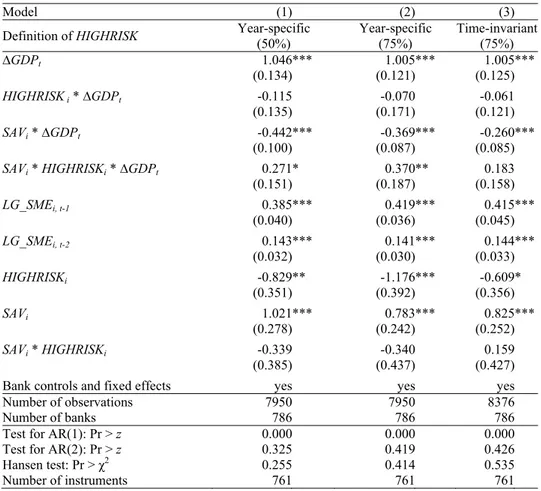
Second, we replace GDP growth with two indicator variables that take on the value of one
in periods with HIGH or LOW GDP growth, respectively, and zero otherwise. We use
Germany’s mean real GDP growth during the sample period as one split criterion to identify
periods with relatively high or low growth, and GDP growth = 0% as another split criterion to
identify periods with absolute growth or decline. This analysis makes it possible to examine
whether the reduced cyclicality in SME lending is symmetric through the cycle or
asymmetric, i.e., only present in certain phases of the economic cycle. Table 4 presents the
results.
In column 1 of Table 4 we use the mean real GDP growth rate as a split criterion for
HIGH and LOW periods. We find that the growth of SME lending by savings banks is
significantly lower than that of cooperative banks during booms (coefficient of SAVi *
ΔGDP_HIGHt =
-0.389). We further find that the coefficient of SAVi * ΔGDP_LOWt is positive but not
statistically significant. In column 2 of Table 4 we use the 0% as a split criterion and find a
strong and symmetric effect through the business cycle: SME lending by savings banks grows
at a lower rate than that of cooperative banks in periods with positive GDP growth and,
interestingly, it grows even during periods with negative GDP growth. The latter finding
suggests that savings banks are not only less cyclical but counter-cyclical during negative
GDP growth periods. Such behavior may be sustainable because it is symmetric through the
business cycle, leading to an inter-temporal smoothing of credit supply.
9
Table 4: High and low GDP growth
The dependent variable is the real growth rate of loans to SMEs (∆LG_SMEi;t). All models are estimated for the full sample
(1987-2007) using the one-step System GMM estimator introduced by Blundell and Bond (1998) as explained above. GMM
-style instruments are created for our main regressors ∆GDP_HIGHt, ∆GDP_LOWt and their interactions with SAVi. The real
GDP growth rate, which is divided into periods of high growth (∆GDP_HIGHt) and periods of low growth (∆GDP_LOWt),
serves as macro variable. Column (1) shows the results for a mean split and column (2) for a positive/negative split (i.e., at
ΔGDP = 0%). We report robust standard errors using Windmeijer’s (2005) finite sample correction in parentheses below
coefficients. Significance levels *: 10% **: 5% ***: 1%.
Model (1) (2)
Split criterion for HIGH vs. LOW Mean GDP 0%
∆GDP_HIGHt 0.582*** 0.638***
(0.068) (0.083)
SAVi * ∆GDP_HIGHt -0.388*** -0.554***
(0.073) (0.092)
∆GDP_LOWt -0.218 -0.008***
(0.173) (0.539)
SAVi * ∆GDP_LOWt 0.223 1.401**
(0.191) (0.602)
LG_SMEi, t-1 0.391*** 0.347***
(0.027) (0.028)
LG_SMEi, t-2 0.091*** 0.113***
(0.023) (0.024)
SAVi 0.684** 1.567***
(0.267) (0.308)
RIIi,t-1 0.395*** 0.500***
(0.092) (0.093)
RNIRi,t-1 -0.071 -0.080
(0.127) (0.134)
ETAi,t-1 -0.458*** -0.493***
(0.152) (0.162)
LIQTAi,t-1 0.089 0.229***
(0.081) (0.086)
LTLRi,t-1 0.041*** 0.032***
(0.007) (0.007)
IBLRi,t-1 0.023* 0.026*
(0.013) (0.014)
DEPRi,t-1 0.031 0.042**
(0.019) (0.019)
Intercept 6.835*** -8.526***
(1.471) (1.539)
Bank controls and fixed effects yes yes
Number of observations 8376 8376
Number of banks 786 786
Test for AR(1): Pr > z 0.000 0.000
Test for AR(2): Pr > z 0.785 0.767
Hansen test: Pr > χ2 0.419 0.399
Number of instruments 782 782
5
Mechanisms
In this section, we examine possible mechanisms behind the different cyclicality of savings
banks and credit cooperatives. Potential mechanisms are bank size, loan maturity structure,
funding structure and liquidity. First, one could argue that SME lending by smaller banks is
volatile over time than the country-wide economy. However, our main result (i.e., savings
banks are on average significantly less cyclical than cooperative banks) in combination with
the fact that the average savings bank is almost twice as big as the average cooperative bank
speaks against this reasoning. We nevertheless carry out a formal test of a potential size
effect. Note that in the previous analysis we normalized all bank variables by total assets but
this procedure does not allow us to directly detect a size effect. To do so, we create size
terciles using average total assets of the savings banks (AVGSIZEi). We interact these size
terciles with the SAVi * ∆GDPt variable. The resulting triple interaction term informs us
whether the lower cyclicality of savings banks is driven by savings banks in a particular size
tercile. The comparison group in this regression is the average sized cooperative bank. We conduct the same analysis for banks’ average long-term loan ratio (AVGLTLRi) to examine
whether maturity structure matters and whether banks’ share of deposit funding
(AVGRELDEPi) are potential channels through which lower cyclicality can be achieved. We
also investigate whether bank liquidity (AVGLIQTAi) is a potential channel. Table 5 presents
the results.
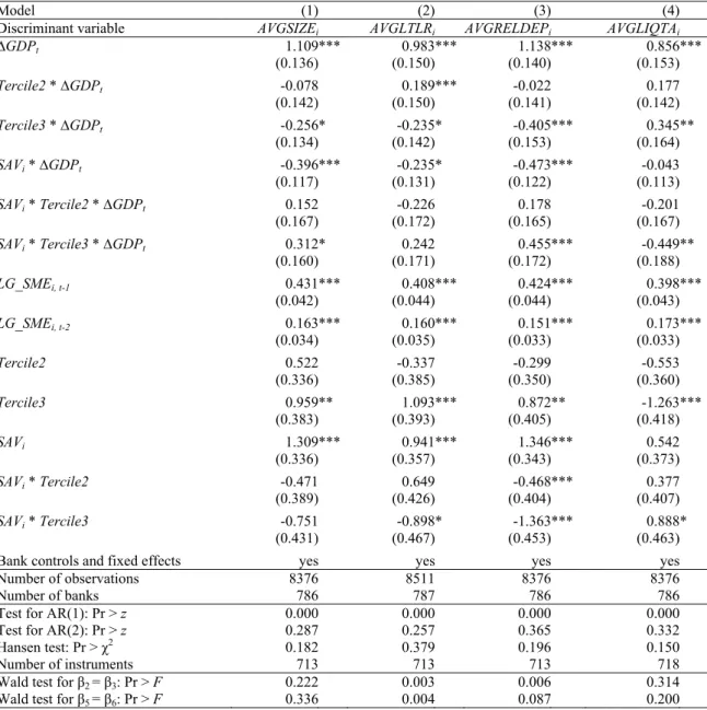
In column 1 of Table 5, the coefficient of the interaction term SAVi * ∆GDPt is
significantly negative, confirming our baseline result for the savings banks from Tercile 1.
The coefficient of the triple interaction term with Tercile 2 is positive, but not statistically
significant, but the one for Tercile 3 is significantly positive. This finding indicates that the
average effect is also present at mid-sized savings banks, and to a smaller extent at larger
savings banks.
In column 2 of Table 5 we study whether loan maturity might be a channel through which
savings banks achieve lower cyclicality. We differentiate by savings banks’ average
long-term loan ratio (AVGLTLRi) and find that the lower cyclicality of savings banks cannot be
explained with the maturity structure of bank lending. The coefficients of the triple interaction
terms (with Tercile 2 and 3) are not statistically significant, but their difference is (p-value of
0.004). This result indicates that the lower cyclicality is not due to a higher fraction of
long-term lending by savings banks compared to cooperative banks. Instead, there are differences
in the loan maturity structure within the savings banks sector.
In column 3 of Table 5 we investigate whether the bank funding structure, in particular
banks’ reliance on deposit funding - compared to wholesale funding - is a channel to achieve
lower cyclicality in lending. We differentiate by savings banks’ share of deposit funding relative to overall funding. Similar to the test for bank size effects (column 1) we find that the
coefficient of the triple interaction term is positive and not statistically significant for Tercile
2, but it is significantly positive for Tercile 3 (banks with the highest share of deposit
funding). The difference between both triple interaction terms is weakly statistically
Table 5: Results by bank size, loan maturity, funding structure, and liquidity
The dependent variable is the real growth rate of loans to SMEs (∆LG_SMEi;t). All models are estimated using the one-step
System GMM estimator introduced by Blundell and Bond (1998), where bank-specific fixed effects are purged by the forward
orthogonal deviations transformation of GMM–type instruments. These instruments are created for our main regressors
LGi;t-2, ∆GDPt and their interaction terms. We study the impact of four bank characteristics (size: AVGSIZEi, long-term lending: AVGLTLRi, deposit funding: AVGRELDEPi, and liquid assets: AVGLIQTAi). We create dummy variables for banks in the
lower, mid and upper tercile (Tercile1, Tercile2 and Tercile3), which we interact with ∆GDPt and SAVi. In order to bring the
number of instruments in line with our finite sample size, the number of lags used is limited accordingly. Furthermore, we
create a collapsed set of GMM–type instruments for the control variables RIIi;t-1, ETAi;t-1, LIQTAi,t-1, LTLRi,t-1, IBLRi,t-1 and
DEPRi;t-1. We report robust standard errors using Windmeijer’s (2005) finite sample correction in parentheses below coefficients. Significance levels *: 10% **: 5% ***: 1%.
Model (1) (2) (3) (4)
Discriminant variable AVGSIZEi AVGLTLRi AVGRELDEPi AVGLIQTAi
∆GDPt 1.109*** 0.983*** 1.138*** 0.856***
(0.136) (0.150) (0.140) (0.153)
Tercile2 * ∆GDPt -0.078 0.189*** -0.022 0.177
(0.142) (0.150) (0.141) (0.142)
Tercile3 * ∆GDPt -0.256* -0.235* -0.405*** 0.345**
(0.134) (0.142) (0.153) (0.164)
SAVi * ∆GDPt -0.396*** -0.235* -0.473*** -0.043
(0.117) (0.131) (0.122) (0.113)
SAVi * Tercile2 * ∆GDPt 0.152 -0.226 0.178 -0.201
(0.167) (0.172) (0.165) (0.167)
SAVi * Tercile3 * ∆GDPt 0.312* 0.242 0.455*** -0.449**
(0.160) (0.171) (0.172) (0.188)
LG_SMEi, t-1 0.431*** 0.408*** 0.424*** 0.398***
(0.042) (0.044) (0.044) (0.043)
LG_SMEi, t-2 0.163*** 0.160*** 0.151*** 0.173***
(0.034) (0.035) (0.033) (0.033)
Tercile2 0.522 -0.337 -0.299 -0.553
(0.336) (0.385) (0.350) (0.360)
Tercile3 0.959** 1.093*** 0.872** -1.263***
(0.383) (0.393) (0.405) (0.418)
SAVi 1.309*** 0.941*** 1.346*** 0.542
(0.336) (0.357) (0.343) (0.373)
SAVi * Tercile2 -0.471 0.649 -0.468*** 0.377
(0.389) (0.426) (0.404) (0.407)
SAVi * Tercile3 -0.751 -0.898* -1.363*** 0.888*
(0.431) (0.467) (0.453) (0.463)
Bank controls and fixed effects yes yes yes yes
Number of observations 8376 8511 8376 8376
Number of banks 786 787 786 786
Test for AR(1): Pr > z 0.000 0.000 0.000 0.000
Test for AR(2): Pr > z 0.287 0.257 0.365 0.332
Hansen test: Pr > χ2 0.182 0.379 0.196 0.150
Number of instruments 713 713 713 718
Wald test for β2 = β3: Pr > F 0.222 0.003 0.006 0.314
Wald test for β5 = β6: Pr > F 0.336 0.004 0.087 0.200
the average credit cooperatives. This finding is plausible because, on average, cooperative
banks exhibit a higher deposit funding ratio than savings banks (see Table 1).
In column 4 of Table 5 we investigate whether bank liquidity affects the cyclicality of
SME lending. Higher liquidity might make it possible for savings banks to better follow their
et al. (2011, p. 569). We find a very strong and significant coefficient for savings banks in
Tercile 3 (-0.449; highest liquidity ratio), while the baseline effect (-0.043) and the interaction
term with Tercile 2 (-0.201) display the expected negative sign but are not statistically
significant. This result provides an important additional insight: Our baseline result becomes
much stronger for savings banks that have sufficient liquidity to be able to lower the
cyclicality of their credit supply to SMEs.
Table 5 indicates that our main result is most pronounced for savings banks with the
highest deposit funding and savings banks with the highest liquidity, respectively. This
finding suggests that the degree of deposit funding and the liquidity situation might be the key
mechanisms behind the lower cyclicality of savings banks’ SME lending. We therefore carry out one additional test. We check whether differences in the sensitivity of deposits and
liquidity to GDP growth between savings banks and cooperative banks can serve as
mechanisms that enable savings banks to provide SME lending in a less cyclical way than
cooperative banks. In these tests we re-estimate the baseline model from Table 2 with
percentage changes in deposits and percentage changes in liquidity as dependent variables,
respectively. The right-hand side of the models is the same as in Table 2. Table 6 presents the
results.
We obtain two clear results. Column 2 of Table 6 shows that savings banks’ deposits are
less cyclical than those of cooperative banks. The coefficient of the interaction term SAVi * ∆GDPt is -1.483 and highly significant. Similarly, column 1 of Table 6 indicates that the liquidity of savings banks is less cyclical than that of cooperative banks. The coefficient of the interaction term SAVi * ∆GDPt is -0.195 and highly significant. Both results are consistent
with the findings shown in columns 3 and 4 of Table 5 and suggest that deposit funding and
the liquidity of assets are mechanisms behind the lower cyclicality of savings banks’ SME
lending. They are able to achieve a lower cyclicality in SME lending than cooperative banks
because they take advantage of less cyclical deposit funding and liquidity, respectively.
6
Additional checks and alternative explanations
In this section, we present several additional tests to rule out alternative explanations. We first
investigate the role of competition for the cyclicality of SME lending. We then rule out that our results are driven by local politicians exerting influence on the lending behavior of
savings banks. Finally, we analyze whether differences in the risk-taking behavior of
cooperative and savings banks can explain our findings.
6.1
Credit supply and bank competition
We first provide a more direct examination of the question as to whether the lower cyclicality
Table 6: Mechanisms behind the lower cyclicality of savings banks
The dependent variable in column (1) is the percentage change in banks’ liquid assets (∆Liqi,t) and the dependent variable in
column (2) is percentage change in banks’ deposits (∆Depi,t) All models are estimated using a least-squares methodology
with bank-level and interacted year*region fixed effects. We report robust standard errors in parentheses below coefficients. Significance levels *: 10% **: 5% ***: 1%.
Model (1) (2)
Dependent variable ∆Liqi,t ∆Depi,t
∆GDPt 4.457*** 0.083
(0.906) (0.105)
SAVi * ∆GDPt -1.483*** -0.195***
(0.533) (0.066)
RIIi, t-1 -5.697*** 0.236
(1.445) (0.224)
RNIRi, t-1 -0.154 0.402***
(0.747) (0.096)
ETAi, t-1 -0.685 0.003
(0.858) (0.191)
LIQTAi, t-1 -0.090
(0.075)
LTLRi, t-1 0.097 -0.015*
(0.065) (0.008)
IBLRi, t-1 0.304*** -0.036***
(0.088) (0.012)
DEPRi, t-1 0.025
(0.110)
Bank-level fixed effects yes yes
Year*region fixed effects yes yes
Number of observations 9403 9403
Number of banks 788 788
R-squared (within) 0.156 0.217
demand-side effect could come from differences in the borrower structure of savings banks
and cooperative banks. If savings banks lend to local borrowers that exhibit a less cyclical
demand for credit than those of cooperative banks, then our findings might not be driven by
the public mandate of savings banks but rather a selection effect in borrower clienteles.
However, the main hypothesis of this study is that the credit supply of savings banks to SMEs
is less cyclical because of their goal to provide sustainable credit to the local economy and their deviation from strict profit maximization (as expressed by the “public mandate” in their
by-laws).
The previous results already indicate that the difference in lending cyclicality between
savings and cooperative banks is a supply-side effect. First, when we include region*year
fixed effects to control for time-varying regional demand for credit this does not affect our
findings. Second, when we use the credit demand-related indicator for Germany from the
European Central Bank’s Bank Lending Survey instead of GDP growth (column 4 of Table 3)
we obtain the same result as in our baseline analysis. Third, savings banks and credit
cooperatives in Germany have been competing in the same regions for the same borrowers for
(i.e., these banks are not allowed to lend to borrowers situated out of their home market). In
addition, the “Borrowers statistics” on the German banking system (Deutsche Bundesbank,
2009) suggest that the industry composition of these banks’ lending portfolios is very similar.
We nevertheless provide this additional test that helps rule out that differences in credit
demand drive our findings. In this test, we take advantage of the cross-sectional and
inter-temporal variation in bank competition to identify whether the lower cyclicality of savings
banks is credit supply-side or credit demand-side driven. We split our sample in observations
with high and low bank competition. It is likely that the observed credit volume is more
closely related to the credit supply function rather than the credit demand function when the
bargaining power of local banks vis-à-vis their borrowers is high. Bank bargaining power is high when local bank competition is low because borrowers have fewer alternatives to obtain
credit (e.g., Petersen and Rajan, 1995). If the lower cyclicality of savings banks is a credit
supply-side effect, then we should observe that this effect is stronger (i.e., savings banks are
even less cyclical) when bank competition is low. To test this prediction, we augment our
baseline model (column 4 of Table 2) by adding the triple interaction term SAVi * logHHIc,t *
ΔGDPt (or: SAVi * COMP3c,t * ΔGDPt; SAVi * COMP5c,t * ΔGDPt), in which we use the Herfindahl-Hirschmann Index (HHI) or concentration ratios C3 and C5, respectively, as
measures of regional bank competition.10 Recall that higher values of the HHI and the
concentration ratios indicate lower bank competition. Based on the above reasoning we
expect to find a significantly negative coefficient of this triple interaction term if the lower
cyclicality of savings banks is a deliberately chosen supply side effect and not due to differences in credit demand. Table 7 reports the results.
In column 1 of Table 7 we find a negative and highly significant coefficient of the triple
interaction term SAVi * logHHIc,t * ΔGDPt (-0.325). We obtain similar results for the triple
interaction terms with the concentration ratios C3 and C5 in columns 2 and 3 of Table 7.
These results indicate that savings banks are even less cyclical in their SME lending than
cooperative banks when bank competition is low. This finding together with the evidence
presented above suggests that our main result is related to the credit supply function of
savings banks, which is ultimately defined by the public mandate in their by-laws, and not
driven by differences in credit demand affecting savings and cooperative banks differently.
6.2
Political influence
We next investigate the role of political influence on the cyclicality of savings banks in more
detail. One could argue that because of their important role as board members in controlling
and supervising savings banks’ activities, local politicians use savings banks to expand
lending in election periods to increase the likelihood of becoming re-elected, and that this is
10
Table 7: Cyclicality and bank competition
The dependent variable is the real growth rate of loans to SMEs (∆LG_SMEi;t). Model 1 corresponds to specification (4) of
Table 2 and we apply the one-step System GMM estimator introduced by Blundell and Bond (1998) as explained above. The
real GDP growth rate (∆GDPt) serves as macro variable. GMM-style instruments are created for our main regressors LGi;t-2,
∆GDPt, and their interactions with the savings banks dummy (SAVi) and a measure for competition at the level of federal
states in Germany. This is the natural logarithm of the Herfindahl-Hirschman Index (logHHIc,t) in Model 1, the concentration
ratio based on the top 3 banks (COMP3c,t) in Model 2 and the concentration ratio based on the top 5 banks (COMP5c,t ) in
Model 3. We report robust standard errors using Windmeijer’s (2005) finite sample correction in parentheses below coefficients. Significance levels *: 10% **: 5% ***: 1%.
Model (1) (2) (3)
Competition measure
Herfindahl-Hirschman Index
Concentration ratio (top 3)
Concentration ratio (top 5)
∆GDPt 0.991** 0.702*** 0.725***
(0.408) (0.213) (0.278)
SAVi * ∆GDPt 1.321*** 0.208 0.246
(0.486) (0.166) (0.191)
logHHIc,t * ∆GDPt -0.014
(0.086)
COMP3c,t * ∆GDPt 1.247
(0.866)
COMP5c,t * ∆GDPt 0.832
(0.951)
SAVi * logHHIc,t * ∆GDPt -0.325***
(0.103)
SAVi * COMP3c,t * ∆GDPt -1.706**
(0.699)
SAVi * COMP5c,t * ∆GDPt -1.432**
(0.618)
LG_SMEi, t-1 0.442*** 0.447*** 0.454***
(0.044) (0.043) (0.044)
LG_SMEi, t-2 0.170*** 0.146*** 0.137***
(0.032) (0.031) (0.031)
SAVi -2.502** 0.359 -0.289
(1.106) (0.415) (0.464)
logHHIc,t 0.173
(0.274)
COMP3c,t -6.696***
(2.336)
COMP5c,t -5.802**
(2.320)
SAVi * logHHIc,t 0.667***
(0.229)
SAVi * COMP3c,t 2.525*
(1.466)
SAVi * COMP5c,t 2.240*
(1.315)
Intercept -8.033** -4.330 -4.297
(3.589) (3.658) (3.624)
Bank controls and fixed effects yes yes yes
Number of observations 7079 7921 7921
Number of banks 621 782 782
Test for AR(1): Pr > z 0.000 0.000 0.000
Test for AR(2): Pr > z 0.164 0.953 0.788
Hansen test: Pr > χ2 0.437 0.241 0.343
the fundamental driver of the differences in lending cyclicality between savings banks and
credit cooperatives. Political influence on lending behavior of public banks has been widely
documented in the literature (e.g., La Porta et al., 2002; Sapienza, 2004; Dinç, 2005;
Carvalho, 2014). As described earlier, most of these studies focus on large public banks that
are owned or controlled by central governments, hence, their settings are not closely
comparable to ours.
In our setting, it is unlikely that political influence plays a role in explaining our main
result. If political influence affects the lending behavior of savings banks, we should expect to
see an expansion of the lending volume in election years, for instance, to please voters. Such
politically motivated expansion of bank lending should be asymmetric: it should take place in recessions but not in booms.
We can rule out this explanation for three reasons. First, political influence does not
explain why savings banks increase their lending volume less than private cooperative banks
in booms. Second, municipal elections take place every four to five years in Germany, but
they are not scheduled simultaneously. There is no systematic correlation between the
occurrence of election years and the state of the economy as reflected by the GDP growth.
Hence, political influence cannot explain why savings banks are less cyclical on average.
Third, the analysis reported in Table 4 shows that the lower cyclicality is due to a symmetric
(and not an asymmetric) lending behavior of savings banks: they expand credit less in booms
and they contract credit less in recessions.
We nevertheless provide a direct test as to whether and how the differences in the lending cyclicality of savings banks and cooperative banks can be explained with political influence
on savings banks. We collect information about the years in which municipal elections take
place during our sample period.11 We create a dummy variable ELECTIONc,tthat equals one if
a municipal election takes place in the county in which the respective bank is located in that
year. We interact this dummy variable with the savings banks dummy and GDP growth (SAVi
* ∆GDPt * ELECTIONc,t) and add all other necessary terms to the baseline regression model
as additional controls. The results are reported in Table 8.
Most importantly, in column 1 of Table 8 we find a positive and significant coefficient for ∆GDPt and a significantly negative coefficient for SAVi * ∆GDPt, confirming our baseline result that savings banks are less cyclical than cooperative banks. We also obtain a
significantly negative coefficient for SAVi * ∆GDPt * ELECTIONc,t. Crucially, this triple interaction effect does not reduce the baseline effect of SAVi * ∆GDPt but it rather comes on
top of it. In column 2 of Table 8 we exclude election years from our sample and test whether
11