Todos os direitos reservados.
É proibida a reprodução parcial ou integral do conteúdo
deste documento por qualquer meio de distribuição, digital ou
impresso, sem a expressa autorização do
Bank Privatization and Market Structure of the
Banking Industry: Evidence from a Dynamic
Structural Model
Fabio Miessi Sanchesy
Daniel Silva Junior
Sorawoot Srisumax
Bank Privatization and Market Structure of the
Banking Industry: Evidence from a Dynamic Structural Model
Fabio Miessi Sanchesy
Daniel Silva Junior
Sorawoot Srisumax
Bank Privatization and Market Structure of the
Banking Industry: Evidence from a Dynamic Structural
Model
∗
Fabio Miessi Sanches
†Daniel Silva Junior
‡Sorawoot Srisuma
§May 25, 2015
Abstract
This paper examines the effects of bank privatization on the market structure of the banking industry. A dynamic game between Brazilian public and private banks is estimated. We show that profits of private banks are positively affected by the number of public banks and negatively affected by the number of private banks operating in small isolated markets. We used the model to analyze two counterfactual scenarios. In the first, public banks are privatized; in the second public banks are closed. Both counterfactuals predict a significant drop in the number of bank branches operating in small isolated markets.
∗Previously circulated under the title “Public Banks Improve Private Banks Performance: Evidence from
a Dynamic Structural Model”. We are indebted to Martin Pesendorfer for his support and guidance during this project. We would like to thank Dimitri Szerman for the help with the data and for insightful comments on several versions of this draft. Robinson Silva helped us to organize the data. We also benefited from discussions with Bernardo Guimarães, Bruno Rocha, Emmanuel Guerre, Fabio Pinna, Francesco Caselli, Francisco Costa, Gabriel Garber, Jason Garred, Joachim Groeger, Johannes Spinnewijn, Maitreesh Ghatak, Matthew Gentry, Michael Dickstein, Panle Jia, Pasquale Schiraldi, Pedro Carvalho, Robert Miller and Tim Besley. Fabio gratefully acknowledges the financial support from CAPES (Brazilian Ministry of Education) and Daniel gratefully acknowledges the support from CNPQ (Brazilian Ministry of Science and Technology). The usual disclaimer applies.
†Department of Economics, University of São Paulo, Brazil. E-mail: [email protected].
‡Department of Economics, London School of Economics and Political Science, UK. E-mail:
1
Introduction
The discussion about the existence of public, state owned banks has been prominent in the banking literature since the 1960’s - see Barth, Caprio and Levine (2001) and La Porta, López-de-Silanes and Shleifer (2002) and Levy Yeyati, Micco and Panizza (2007). Advocates of public banks argue that they provide financial access to populations living in areas that are unattractive for private institutions, fostering financial development. Critics of public banks argue that they crowd-out more efficient, more competitive private banks, slowing down the development of the financial system.
This paper examines how the existence of public banks affects the structure of the banking industry in small isolated markets. A dynamic entry game between Brazilian public and private banks is estimated. We used the model to analyze two counterfactual scenarios. In the first public banks are privatized; in the second public banks are closed. We analyze the effects of these policies on the number of bank branches operating in small isolated markets. Three main conclusions emerge. First, public banks generate positive profit spill-overs for private banks. Second, private banks crowd-out private competitors. Third, the counterfac-tual in which public banks are sold to private banks shows that the average number of bank branches in a typical small isolated market drops from 1.9 to 0.43. In the counterfactual where public banks are closed (excluded from the market) the number of branches drops from 1.9 to 0.3. Under both counterfactual scenarios most of the small isolated markets would end up without any bank branch.
These findings have important policy implications in developing countries. In these coun-tries a large fraction of the population has no access to the banking market. Yet the access to financial services generates positive effects in terms of poverty reduction and economic growth in disadvantaged areas (Burgess and Pande (2005) and Pascali (2012)).
This paper builds a dynamic entry game between Brazilian public and private banks. The dynamic structure of the model is rationalized by the existence of substantial entry costs in the market. At each period these banks have information about the state variables and decide simultaneously to be active or not active in a given market by maximizing an inter-temporal profit function. Entrants pay a entry cost. We assume that the profit function of private banks is asymmetrically affected by public and private competitors.
We use data from isolated markets in Brazil during 1995-2010 to estimate the decision rules for public and private banks. We analyze two different structural models. The first is stationary and has finite state space. The second model is non stationary. The non stationary model allows some state variables to grow continuously over time and admits equilibrium choice probabilities that are time dependent. Our models account for time and market unobservables. We recover the primitives of the game that are consistent with the estimated decision rules. The model is solved for the entry probabilities. The market equilibrium is evaluated under a counterfactual scenario where public banks are privatized1 and under
a counterfactual scenario where public banks are closed2. Our results assume that payoff
parameters are invariant to the policy change. We report consistent ex ante estimates of the effects of these policies on market outcomes. Our model is valuable to predict policy changes.
Methodologically our paper is related to the empirical industrial organization literature that studies the estimation of dynamic games - see Aguirregabiria and Nevo (2010), Ba-jari, Hong and Nekipelov (2010) and Pesendorfer (2010) for a rich discussion on the topic. Applications that are similar to ours are also found in Pesendorfer and Schmidt-Dengler (2003) for small businesses in Austria, Dunne, Klimek, Roberts and Xu (2013) for dentists and chiropractors in the US, Gowrisankaran, Lucarelli, Schmidt-Dengler and Town (2010) for hospitals in the US, Collard-Wexler (2013) for the concrete industry in the US, Ryan (2012) for the cement industry in the US and Kalouptsidi (2014) for the shipping industry. Other related applications include Maican and Orth (2012), Minamihashi (2012), Lin (2011), Fan and Xiao (2012), Nishiwaki (2010), Arcidiacono, Bayer, Blevins, and Ellickson (2015), Jeziorski (2014), Snider (2009), Suzuki (2012), Sweeting (2013), Beresteanu, Ellickson and Misra (2010) and Igami (2014).
To estimate our models we use the Asymptotic Least Squares (ALS) estimator proposed
1
This counterfactual reflects the case where, after privatization, public banks start to operate based on the policy functions of private banks.
2
in Sanches, Silva and Srisuma (2015a). Sanches, Silva and Srisuma (2015a) show that there can be substantial computational gains when an ALS estimator (in the sense of Gourieroux and Monfort (1995)) is defined in terms of expected payoffs instead of choice probabilities; the latter is developed in the well known paper by Pesendorfer and Schmidt-Dengler (2008)3. An
important feature of the former approach when the payoffs have a linear-in-the-parameters structure their ALS estimators have the familiar OLS/GLS closed-form expression. Closed-form estimation is attractive as it always obtains a global minimizer without any numerical methods in contrast to some well established estimation procedures for dynamic games that rely on nonlinear optimization procedure (e.g. Aguirregabiria and Mira (2007), Bajari, Benkard and Levin (2007) and Pesendorfer and Schmidt-Dengler (2008), among others).
This paper is organized as follows. The next section describes our dataset and the Brazilian banking market. Section 3 provides reduced form evidence of competition be-tween public/private banks. Sections 4 and 5 describe the theoretical model, the empirical model and our main results. Section 6 discusses the fitting of the empirical model and our counterfactual analysis. The last section concludes the paper.
2
Data and Institutional Background
The data comes from the Brazilian Central Bank and from the Brazilian Ministry of Labor. The Brazilian Central Bank database has followed the activities of all Brazilian banks since 1900. These data contain the opening and closing dates4 and the name of the chain that
operates each branch for all branches opened since 1900 in all Brazilian municipalities. A measure of market size is constructed by using data from the Brazilian Ministry of Labor containing the total payroll in the formal sector5 for all Brazilian cities since 1985. The
payroll data is deflated using the official inflation index, IPCA-IBGE. All the values are in R$ of 2011. The information about banking and economic activity is annual.
Following Bresnahan and Reiss (1991) our analysis examines small isolated markets. We select municipalities6 that are (i) at least 20 km away from the nearest municipality and (ii)
that are at least 100 km away from state capitals. State capitals and metropolitan areas are
3
Sanches, Silva and Srisuma (2015a) also show that the ALS estimators of Pesendorfer and Schmidt-Dengler (2008) and theirs are asymptotically equivalent so there is no effciency lost for the computational gain.
4
For the branches that were closed. 5
Number and wage of employees in the formal sector of the economy. 6
also excluded7. We also exclude municipalities that have more than 10 bank branches since
19008 and municipalities where the information for entry/exit dates of any bank branch are
missing. This selection leaves us with 1002 isolated small markets, corresponding, roughly, to 20% of all Brazilian municipalites. Isolated markets enable us to obtain a clear measure of the potential demand for each branch.
The data on market size is available from 1985. We exclude the period 1985-1994. This is a period of severe macroeconomic disorganization, including a long period of hyperinflation and a number of unsuccessful heterodox stabilization plans. Our final sample consists of observations for 1002 isolated municipalities in the period 1995-2010. The vast majority of municipalities have either one or none branch per chain. Our initial focus of analysis is therefore on entry and exit patterns.9
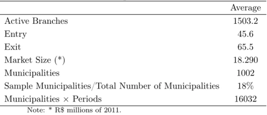
Sample statistics. The next table illustrates the basic statistics of our sample.
Table 1: Basic Sample Statistics 1995-2010 Average Active Branches 1503.2
Entry 45.6
Exit 65.5
Market Size (*) 18.290 Municipalities 1002 Sample Municipalities/Total Number of Municipalities 18% Municipalities×Periods 16032
Note: * R$ millions of 2011.
Our sample is composed by 1002 isolated markets. This corresponds to approximately 18% of the total number of municipalities in Brazil. The number of branches in this sample is 1503 per year on average. Entry is observed 45 times per year and exit 65 times. The average market size measured by the total payroll of the formal workers in a given municipality/year is of R$ 18.3 millions of 2011. This value is relatively small because by excluding state capitals and metropolitan regions, the richest cities in the country are left aside.
7
All these criteria have been used in Bresnahan and Reiss (1991). 8
These municipalities are relatively large, possibly comprising more than one geographic market. It would be difficult to isolated the size and the competitors in each of the different geographic markets in these municipalities.
9
In 2010 our sample had 17 different chains with at least one active branch. The biggest chain in that year was Bank of Brazil (BB), with 670 active branches; the second biggest was Bradesco, with 300 active branches; the thrid largest was Itau with 154 active branches and the fourth largest was Caixa Economica Federal (CEF), with 122 active branches. BB and CEF are public and controlled by the Federal government. The other two, Bradesco and Itau, are privately held.
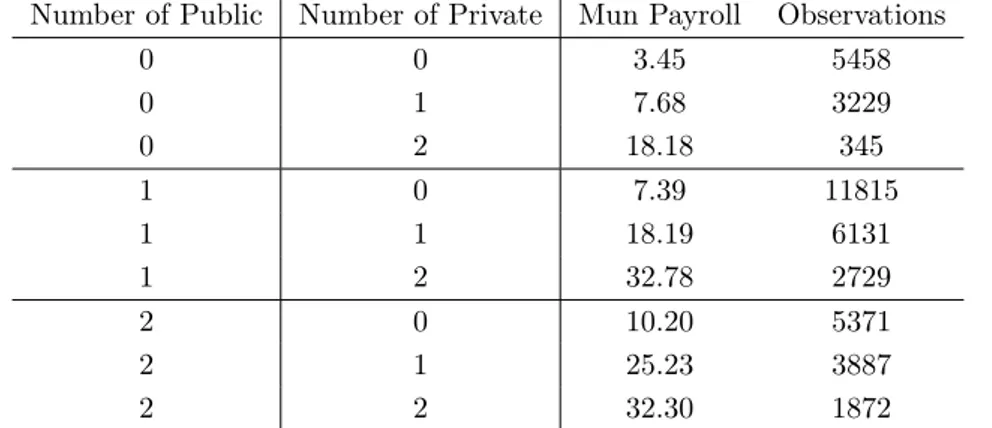
Table 2 reports (i) the frequency distribution of each market configuration (number of ob-servations corresponding to each market structure) and (ii) the average market size (monthly average payroll of the municipality in R$ millions of 2011) corresponding to each market structure. These numbers illustrate that:
1. Public banks are located more frequently in small markets (as measured by the mu-nicipality average payroll) than private banks; and,
2. Public banks are frequently the only providers of financial services in these isolated markets (the frequency of public monopolies - 11815 observations - is the highest in the sample).
Table 2: Average Monthly Payroll and Number of Public/Private Banks Number of Public Number of Private Mun Payroll Observations
0 0 3.45 5458 0 1 7.68 3229 0 2 18.18 345 1 0 7.39 11815 1 1 18.19 6131 1 2 32.78 2729 2 0 10.20 5371 2 1 25.23 3887 2 2 32.30 1872
Note: Average market size is the monthly average payroll of the municipal-ity and is measured in R$ millions of Jan/2011 according to the number of banks in the market. Sample period: 1995-2010. Each observation cor-responds to a municipality in a given year. We showed in the table only the most frequent market structures. This corresponds to around 80% of the total number of observations.
financial services) is quite high in our sample. In addition, the empirical evidence indicates that public banks are much less productive than their private counterparts (Nakane and Weintraub (2005)). This means that the presence of public banks in smaller markets is not explained by cost advantages of public banks.
Institutional background. The Brazilian banking market is large. In 2012 Itau was
considered the 8th largest bank in the world in terms of market value (with a market value of US$88 billions); Bradesco was the 17th largest (market value of US$64 billions) and Bank of Brazil was the 31st largest (market value of US$42 billions)10.
As Coelho, Melo and Rezende (2012) point out, there are important differences in the objectives of public and private banks. Private banks are essentially profit oriented. By legal mandate, public banks focus their operations on market segments that are not profitable for private banks. This suggests the existence of product differentiation in the market. In what follows we describe the “social” role of public banks in Brazil.
BB has expanded enormously its operations in smaller and poorer areas of the country based on central government policies aiming to “popularize” banking services among poor workers and small businesses. BB plays an important role as the provider of government funds to the Brazilian agriculture11. Also, to expand its capillarity in isolated areas, BB
created a DSR (Regional Development Program). The DSR provides a set of tools for small entrepreneurs, including a business plan, technical support and credit12.
CEF has a monopoly over a number of different government funds and services, such as the FGTS, Bolsa Família, PIS13 and the Federal Lottery14. FGTS is a Brazilian fund
created in 1966 to provide assistance to unemployed people15 . These resources are allocated
in two main areas: housing and sanitation. The government gives the investments guidelines
10
http://www.relbanks.com/worlds-top-banks/market-cap. Access: November 12, 2012. 11
The total amount of agricultural credit provided by this bank in 2010 reached more than US$ 26 billions. Moreover, BB is the main bank in the Pronaf, a program created to supply credit for small businesses (agriculture, fishing, tourism, and handcraft) in rural areas at a very low interest rate. The total credit availble for the program increased from US$ 1 billion in 1999 to US$ 7 billions in 2010. All banks in Brazil are allowed to take part in the program, however, BB distributes around 65% of the total Pronaf credit.
12
In 2007 the program supported 2800 business plans and distributed US$ 1.7 billions in credit. 13
PIS is a tax to cover unemployment benefits. Their assets were around US$14 billions in December 2010. 14
The Federal Lottery provided a gross revenue of US$5.2 billions in 2010. It is used to fund sports. 15
in order to finance strategic areas with lack of credit. CEF is also responsible for the distribution of the benefits from Bolsa Família16, a program that gives to poor families a
monthly income. It was created to reduce the poverty in the most backward areas of the country.
3
Reduced Form Analysis
We estimate a series of reduced form linear probability models to explain activity decisions of public and private banks using the sample of isolated municipalities.
Two linear probability models are estimated: one for public banks, the other for private banks. In the model for public banks we pool all public banks. To estimate the model for private banks we pool all private banks.
Our specification is:
atim=
ρ0+ρ1at− 1
im +ρ2npub,t− 1
m +ρ3npri,t− 1
m +ρ4xtm+µ
t
+µim+µtm+ζ t
im. (1)
The dependent variable, at
im, is the action of bank i in municipality m, period t. It
assumes 1 if bank i was active in that municipality/period and zero otherwise. at−1
im
indi-cates the action of the same bank in that municipality in the prior period. npub,t−1
m is the
number of public competitors in the previous period in market m17; npri,t−1
m is the number
of private competitors in the previous period in marketm18; xt
m is a vector of municipality characteristics; µt are time effects; µ
im are market/bank specific effects and µtm captures
market/time specific effects and ζt
im is an idiosyncratic term varying across banks, market
and time periods. (ρ0,ρ1,ρ2,ρ3,ρ4) denote coefficients to be estimated. The data include all muncipalities where bank i was active for at least one period19.
16
In 2006 the program served around 11 million families or approximately 44 thousand individuals. The public expenditure with the program is around 0.5% of the Brazilian GDP and is growing steadily since its creation.
17
Mathematically,npub,tm −1=
P
j∈ipub,j6=i
atjm−1, where ipub is the set of public banks.
18
Mathematically,npri,t−1
m =
P
j∈ipri,j6=i
atjm−1, where ipri is the set of private banks.
19
The potential market is defined based on the super efficient estimator described in Pesendor-fer and Schmidt-Dengler (2003). We defined that market m is a potential market for bank i if
max
t {a t
We estimate model (1) using a fixed effects estimator. A fixed effect in this model is
µim, that is, we have a different fixed effect for each bank in each market. The terms µt are
modeled as year dummies and the terms µt
m are modeled as an interaction between a time
trend and market dummies. The vector xt
m includes municipality payroll, transfers of the Federal and State govern-ments to the municipality, municipal government expenditure and agricutural production of the municipality. Municipality payroll is a measure of market size. The inclusion of transfers and municipal expenditure controls for the fact that entry of public banks can be correlated with an increase of Federal/State investment in the municipality, which can also affect entry of private banks. Agricultural production is included because a large fraction of the income in our isolated municipalities comes from agricultural activities. This variable is a different indicator of market size.
3.1
Public banks
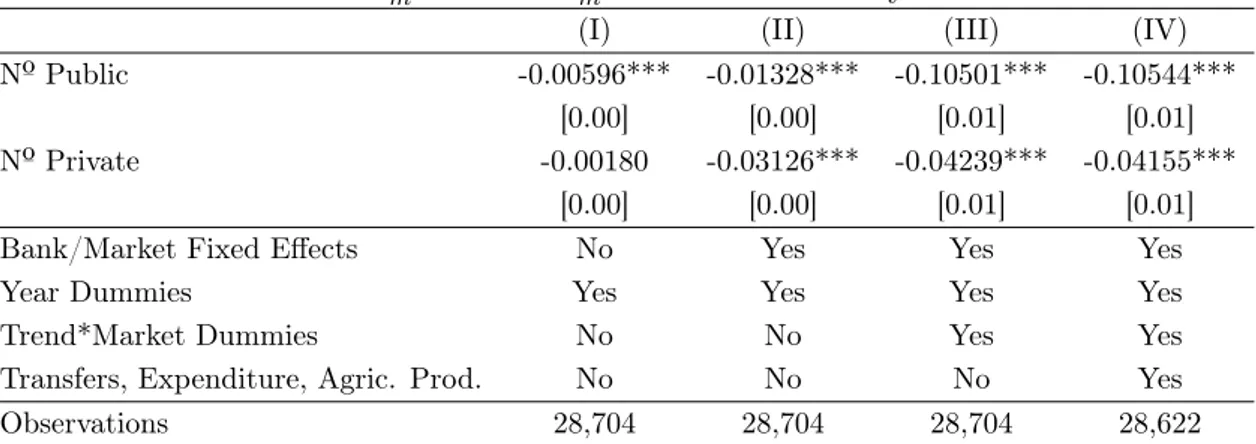
Table 3 reports the estimates of equation (1) for public banks. Only the coefficients associated with npub,t−1
m and npri,t−
1
m are reported. Entry probabilities of public banks are negatively
affected by the number of public and private competitors in the market. These effects become more pronounced when the interaction between market dummies and the time trend are included in the model - columns (III) and (IV). In the specifications with market/bank fixed effects and interaction between market dummies and the time trend a public competitor in the previous period reduces in approximately 10% the activity probabilities of a public bank in the current period; a private competitor in the previous period reduces the activity probabilities of a public bank in 4% in the current period, approximately.
Table 3: Effects of npub,t−1
m and npri,t−
1
m on the Activity of Public Banks
(I) (II) (III) (IV) Nº Public -0.00596*** -0.01328*** -0.10501*** -0.10544***
[0.00] [0.00] [0.01] [0.01] Nº Private -0.00180 -0.03126*** -0.04239*** -0.04155***
[0.00] [0.00] [0.01] [0.01] Bank/Market Fixed Effects No Yes Yes Yes Year Dummies Yes Yes Yes Yes Trend*Market Dummies No No Yes Yes Transfers, Expenditure, Agric. Prod. No No No Yes Observations 28,704 28,704 28,704 28,622
Note: (***) Significant at 1%; (**) significant at 5%; (*) significant at 10%. Clustered standard errors by municipality/bank in brackets. All the models have lagged activity, number of public and private competitors and municipality payroll. Transfers correspond to the total transfers of Federal and State governments to the municipality. Expenditure corresponds to municipal government expenditure. Agricultural Production is the total agricultural production of each municipality.
3.2
Private banks
Table 4 reports the estimates of equation (1) for private banks. The number of public com-petitors increases the activity probabilities of private banks in 0.70%-1.94%. This effect is significant and robust across specifications. The inclusion of market/bank effects and the interaction between market dummies and the time trend increases this effect. In specifica-tions (III) and (IV) the number of private competitors reduces the activity probabilities in approximately 2.7%.
Table 4: Effects of npub,t−1
m and npri,t−
1
m on the Activity Probabilities of Private Banks
(I) (II) (III) (IV) Nº Public 0.01114*** 0.00690** 0.01936*** 0.01892***
[0.00] [0.00] [0.00] [0.00] Nº Private 0.00201 0.04239*** -0.02699*** -0.02785***
[0.00] [0.00] [0.01] [0.01] Bank/Market Fixed Effects No Yes Yes Yes Year Dummies Yes Yes Yes Yes Trend*Market Dummies No No Yes Yes Transfers, Expenditure, Agric. Prod. No No No Yes Observations 22,528 22,528 22,528 22,441
We also investigate whether these results - particularly the positive effect on npub,t−1
m - are
robust against the potential bias that may arise from the estimation of dynamic models with fixed effects; see Nickell (1981)20. To do this, we estimate specification (IV) in Table 4 using
the GMM estimator developed in Blundell and Bond (1998)21.
In the first GMM specification we only have lagged activity,atim−1, in the set of endogenous variables; in the second we haveatim−1, npub,t−1
m andnpri,t
−1
m in the set of endogenous variables.
We use as instruments for the endogenous variables two lags22 of the first difference of these
variables, transfers of the Federal and State governments to the municipality, municipal government expenditure and agricutural production, bank/market dummies, time dummies, and the interaction of the time trend and market dummies.
The results are shown in Table 5. In both models the coefficients associated withnpub,t−1
m
are positive and significant at 1%. They are similar to the fixed effects estimates reported in Table 4. The coefficients associated with npri,t−1
m are also negative and significant at 1%.
Their magnitude, in absolute value, is relatively smaller than the fixed effects estimates. The GMM estimates suggest that the effects ofnpub,t−1
m andnpri,t
−1
m on the entry
probabil-ities of private banks are robust to the Nickell bias and to inconsistency problems caused by the potential endogeneity ofnpub,t−1
m andnpri,t−
1
m . In particular, the coefficient associated with npub,t−1
m remains positive and significant when we explicitly treat this variable as endogenous
- see column (II) in Table 5.
20
Nickell (1981) shows that the estimation of dynamic linear panel data models using fixed effects is generally biased for large “N” and small “T” samples.
21
This estimator is known to be able to produce consistent estimators in dynamic models with fixed effects. 22
Table 5: Effects ofnpub,t−1
m andnpri,t−
1
m on the Activity Probabilities of Private Banks (GMM)
(I) (II)
Nº Public 0.02015*** 0.01956*** [0.00] [0.00] Nº Private -0.02856*** -0.01737***
[0.00] [0.00] Bank/Market Fixed Effects Yes Yes Year Dummies Yes Yes Trend*Market Dummies Yes Yes Transfers, Expenditure, Agric. Prod. Yes Yes Endogenous Variables atim−1 atim−1,npub,t−1
m ,npri,tm −1
Observations 15,897 15,897
Note: (***) Significant at 1%; (**) significant at 5%; (*) significant at 10%. Clustered standard errors in brackets. All the models have lagged activity, number of public and private competitors and municipality payroll. Transfers correspond to the total transfers of Federal and State governments to the municipality. Expenditure corresponds to municipal government expenditure. Agricultural Production is the total agricultural production of each municipality.
4
Theoretical Model
This section sets up and solves a dynamic entry game between Brazilian banks. Motivated by the data, the game considers entry and exit decisions. In the data a chain has typically at most one branch in each municipality23.
The model captures the features documented by the reduced forms. Dynamics can be rationalized by high entry costs24. Importantly, the model allows for different behavior of
public and private banks.
We estimate the primitives that rationalize the behavior of private banks using a dynamic oligopoly game. We follow the literature on public banks and do not structurally model their behavior. This literature recognizes that public banks are not necessarily profit maximizers. The behavior of public banks can depend on political and social reasons - see Levy Yeyati et al (2007), La Porta et al (2002) and Barth et al (2001).
At each period private banks have information about the state variables and decide simultaneously to be active or not active in a given market by maximizing an inter-temporal
23
As described above only in 4% of these municipalities one chain had more than 1 branch during the same period.
24
profit function. Private banks know that the entry of public banks is exogenously given. Private entrants pay an entry cost. The profit function of the private banks is assumed to be asymmetrically affected by public and private competitors. This allows us to understand how public banks influence the performance of private banks.
We analyze two different structural models. The first, which we call baseline model is stationary and has finite state space. Similar models have been employed in Pesendorfer and Schmidt-Dengler (2003), Dunne, Klimek, Roberts and Xu (2013), Gorisankaran, Lucarelli, Schmidt-Dengler and Town (2010), Collard-Wexler (2013), Ryan (2012) and Kalouptsidi (2014), among others.
The second model, which we call alternative model, is non stationary. The non stationary component of the model allows us to control for richer forms of time varying unobserved heterogenity affecting payoffs. It is also consistent with the fact that some variables are growing steadily over time. A similar model has been employed in Igami (2014).
4.1
Baseline model
The assumptions and the equilibrium characterization of the baseline model are outlined below.
4.1.1 Assumptions
Banks. There are Npri > 0 private banks. The set of private banks is indexed by ipri.
There are Npub >0public banks. The set of public banks is indexed by ipub.
Time and markets. Time is discrete, t= 1,2, ...,∞. There are m∈M=1,2,3, .., M
markets.
Actions. A bank’s action in market m, period t is denoted by atim ∈ {0,1}, where 0
means that the bank is inactive; 1 means the bank is active. The 1×(Npri+Npub) vector atm denotes the action profile in market m, period t. We sometimes use at−im to denote the actions of all banks but bank i.
State space. The state space is discrete and finite. We use stm to denote an element of
the state space in market m. When necessary we use Ns to express the number of different
possible states in market m.
Transitions. The vector stm evolves according to the transition matrix pm(smt+1|stm,atm), described by next period distribution of possible values for the vectorst
vector of transitions,pm(stm+1|stm,atm), for every possible future state st +1
m given any possible
(st m,atm).
Unobservables. In each period banks draw a profitability shock εtim. The shock is
privately observed while the distribution is publicly known.
Payoffs. Private banks’ period payoff is:
Π(atm,stm;Θim) =
πm(atm,xtm)
+1(at
im= 1)εtim
+1(atim= 1)1(atim−1 = 0)F.
(2)
Here πm(atm,xtm) denotes private banks’s deterministic profits in market m, F are en-try costs and εt
im is a profitability shock, which will be specified below. Θim denotes the parameters in the model.
This specification captures the main aspects of our idea. A private incumbent deciding to stay in the market receives period profits of πm(atim= 1,a−tim,xtm) +εtim. A private entrant
receives the same profit as an incumbent minus the sunk entry cost F. Any private bank that is outside and considers re-entering the market has to pay a fixed cost25.
The term πm(atm,xtm) is a linear function of exogenous states and actions26:
πm(atm,x t m) =
π0+π
pub
1
X
j∈ipub
atjm
+π
pri
1
X
j6=i,j∈ipri
atjm
+π2xtm
·1(atim= 1). (3)
Here πk ∈ Rk are parameters and xtm is a demand shifter. This specification allows for different “competition” effects of public and private banks.
The profitability shock εt
im is assumed to have two components:
εtim =µim+ξtim, (4)
25
We assume that banks leaving the market get a scrap value equal to zero. Aguirregabiria and Suzuki (2014) and Sanches, Silva and Srisuma (2015b) discuss identification problems of entry costs, scrap values and fixed costs in dynamic entry games.
26
where, µim is a term that varies only across markets and banks but not over time and ξt
im∼EV(0,1)is an idiosyncratic shock iid across banks, time and markets. ξimt is the only
source of asymmetric information in the model. The term µim is known to the banks. It
captures correlation of the profitability shocks for the same bank in the same market across time. The inclusion of µim in (4) is empirically justified by the significance of bank/market
effects in the reduced forms analyzed above. The parameters of interest are Θim =
n
F, π0, π
pub
1 , π
pri
1 , π2, µim
o
. We sometimes denote payoffs as Π(at
m,stm;Θim) = ˜Π(atm,stm)Θim +1(atim = 1)ξimt , where Π(˜ amt ,stm) is a 1×Np
vector and Np is the number of parameters in marketm.
We do not model the behavior of public banks. Actions of public banks are exogenous in the model.
Sequence of period events. The sequence of events of the game is the following:
1. States are observed by private banks.
2. Each private bank draws a private profitability shock εt im.
3. Actions are simultaneously chosen. Private banks maximize their discounted sum of period payoffs given their beliefs on private competitors and public banks actions. Beliefs of private banks on public banks actions are exogenously given. The total payoff of a private bank is given by the discounted sum of bank’s period payoffs. The discount rate is given by β <1 and is the same for all banks.
4. After actions are chosen the law of motion for st
m determines the distribution of states in the next period; the problem restarts.
Next the equilibrium for this game is characterized.
4.1.2 Equilibrium characterization
We restrict attention to pure Markovian strategies. This means that private banks’ actions are fully determined by the current vector of state variables. Intuitively, whenever a private bank observes the same vector of states it will take the same actions and the history of the game until period t does not influence private bank’s decisions.
M ax
at i=k∈{0,1}
P at −im
σim(at−im|stm)Π(aimt =k,at−im,stm;Θim)+
βzk(stm+1|stm;σim,pm)EξVim(σim,pm)
. (5)
Here Π(·) is bank’s period payoff; the function σim(a−tim|stm) accounts for i’s beliefs on other private and public banks’ actions given current states27; σ
im is a vector that con-tains the beliefs for all possible combination actions given any possible state in market m; zk(stm+1|stm;σim,pm)is a1×Nsvector containing the transitionsσim(at−im|stm)pm(stm+1|atim= k,at
−im,stm) and EξVim(σim,pm) is a Ns×1 vector with the expected continuation value
for private bank i in market m, EξVi(stm+1;σim,pm,Θim), for all stm+1.
The conditional value function, conditional on action k ∈ {0,1} being played, is given by:
Vimk stm;σim,pm
=
X
at
−im
σim(at−im|stm) ˜Π(aimt =k,at−im,stm)Θim (6)
+βzk st +1
m |stm;σim,pm
EξVim(σim,pm) +1(k = 1)ξtik.
We also define V˜k
im(stm;σim,pm) = Vimk (stm;σim,pm)−1(k = 1)ξikt as the conditional
value function net of the iid profitability shock, 1(k= 1)ξikt .
We define EξVim(σim,pm) as the ex-ante value function, that is, EξVim(σim,pm) =
∆im
˜
ΠimΘim+E˜ξim
, where∆im = [INs −βZim]
−1
;Π˜im is aNs×Np vector stacking
cur-rent payoff expected values,P
at+1 im
σim(atm+1|st +1 m ) ˜Π(at
+1 m ,st
+1
m ), for everyst +1
m ;E˜ξimis aNs×1
vector stackingE˜ξ(smt+1;σim,pm) =
K
P
k=0
σim(at
+1
im =k|st
+1
m ;σim,pm)E
ξtim+1|atim+1 =k,st+1 m
for
everyst+1
m ;INs is aNs×Ns identity matrix; andZim is aNs×Ns matrix stacking the1×Ns
vector z(st+2 m |st
+1
m ;σim,pm) containing the transitionsσim(atm+1|st +1
m )pm(stm+2|at +1 m ,st
+1
m ) for
every st+1
m .
The solution to problem (5) implies that private bank i’s probability of playing action
k = 1 when states are st
m satisfies the following equilibrium restrictions:
27
Him(ati = 1|s
t
m;σim,pm) =
1−expn−expn V˜1
im(stm;σim,pm)−V˜im0 (stm;σim,pm) oo
. (7)
This holds for all st
m∈Sm and all i∈ipri.
The solution to this problem is a vector of private bank i’s optimal actions when this bank faces each possible configuration for the state vectorst
m and has consistent beliefs about other public and private banks actions in the same states of the world.
By stacking up best responses for every private bank and every state a system of1×Npri· Nsequations in each market can be formed. This system is used to find the1×Npri·Nsvector
of private banks’ beliefs. A formal proof of the existence of this vector can be found, for instance, in Aguirregabiria and Mira (2007) and Pesendorfer and Schmidt-Dengler (2008). Equilibirum uniqueness, however, is not guaranteed. This is a common feature of entry games.
4.2
Alternative model
In the alternative model we assume that time is discrete and finite,t= 1,2, ..., T. Payoffs of private banks are the same as in the baseline model described in (2). The profitability shock
εt
im is modeled as:
εtim =µim+η·t+ξimt .
Here, t is a time trend assuming values on t ∈ {1,2, ..., T}. This component allow us to control for a more flexible form of time varying unobserved heterogeneity affecting private bank’s decisions. The components µim and ξtim are the same as in the baseline model.
The time varying shock is included to capture the fact that the decision structure of the chains can be centralized. First, the “general” conditions of the economy are observed. Second, the decision in which municipality(ies) to enter/exit is taken. The model captures the feature that a better (worse) macroeconomic landscape can increase (decrease) the prob-ability of being active in all available markets.
We further assume thatxt
m, the demand shifter in private banks’ payoffs, evolves following
a deterministic rulext+1
m = (1 +γxm)·xmt , whereγxm is the long-run growth rate ofxtm. This
be growing steadily over time. The evolution of the trend across time is also deterministic. Because of these components the model is non stationary. This version of the model is similar to the one used in Igami (2014).
As before, we do not structurally model the behavior of public banks. Public banks are taken to be exogenous. The sequence of events faced by the banks is the same as the baseline model. Because of the finite time horizon feature of the game, it can be solved backwards as in Igami (2014).
5
Econometric Model
This section describes identification and the estimation procedure. The identification of the models we consider can be studied following Pesendorfer and Schmidt-Dengler (2008). Our estimation procedure follows the OLS approach suggested in Sanches, Silva an Srisuma (2015a).
5.1
Identification
Following the CCP approach (Hotz and Miller (1993)) we firstly identify the vector of activity probabilities for public and private banks and the transitions directly from the data. For the identification of activity probabilities we need to introduce two assumptions:
Assumption (i): There are no unobserved common knowledge states.
Assumption (ii): The same equilibrium is played in all available markets.
These identifying assumptions follow Ryan (2012). Pesendorfer (2010), Aguirregabiria and Nevo (2010) and Bajari, Hong and Nekipelov (2010) discuss the importance of the assump-tions above.
Assumption (i) can be somewhat relaxed as illustrated in Arcidiacono and Miller (2011). However, this makes the estimation problem and counterfactual analysis substantially more difficult. Our structural models already include bank/market and time fixed effects. This mitigates our concern with unobservables.
exit movements within each market to accurately identify the reduced form parameters sepa-rately. Therefore it is necessary to pool data of different markets in our application. Pooling of data across markets is necessary in several related empirical games in the literature, e.g. Collard-Wexler (2013) and Ryan (2012).
Under these assumptions the identification of period payoff parameters follows from re-sults in Pesendorfer and Schmidt-Dengler (2008).
5.2
Estimation: Baseline model
We use the estimation principle suggested in Sanches, Silva and Srisuma (2015a) to recover banks’ payoffs. We start by representing the equilibrium restrictions (7) as a linear function of the payoff parameters. By inverting the function on the LHS of (7) and substituting
˜ V1
im(stm;σim,pm) and V˜im0 (stm;σim,pm) equation (7) can be written as:
y(stm;σim,pm)−D(stm;σim,pm)Θ
′
im = 0, (8)
where, y(st
m;σim,pm) is a real valued differentiable function that depends only on states, beliefs and state transitions and D(st
m;σim,pm)is a real valued 1×Np vector that depends
only on states, beliefs and state transitions. These functions are defined in the appendix. As in Pesendorfer and Schmidt-Dengler (2008) we assume that {(ˆσim,ˆpm)}m∈M are
con-sistent and asymptotically normal estimators for the beliefs and state transitions in all the markets. We defineyˆimt =y(smt ;ˆσim,pˆm)andDˆimt=D(stm;ˆσim,ˆpm)and sum and subtract
ˆ
yimt−DˆimtΘ
′
im from (8) to write:
ˆ
yimt =DˆimtΘ
′
im+ ˆuimt, (9)
where, uˆimt =
ˆ
yikmt−DˆimtΘ
′
im
− yimt−DimtΘ
′
im
, with yimt = y(simt ;σim,pm) and
Dimt =D(stm;σim,pm).
By stacking equation (9) for all the markets, states and private banks OLS can be used to recover Θ′im. Sanches, Silva and Srisuma (2015a) show that the OLS estimator is consistent and has an asymptotic normal distribution when the sample size tends to infinity.
Following the CCP approach the empirical implementation of our model depends on (i) the estimation of beliefs and actions for each bank, respectively, Him(ati = 1|stm;σim(·)) and σim(at−im|smt )and (ii) the estimation of a transition process for the exogenous states, psm(·).
Firstly, there are markets in our sample with a different number of potential public and private banks28. N
pri and Npub vary significantly across markets. We cannot pool
markets with different number of potential players as equilibrium in these markets will be intrinsically different29. We are interested in understanding how the interaction between
private-private, private-public and public-public banks affects the structure of the banking market. Therefore, we estimate the CCPs of private banks pooling data of markets where
Npri = 2 and Npub = 2. In total we have 46 markets with this configuration. We estimate
the CCPs using a logit model.
Market/bank fixed effects are also included in the logit model. Because of the inci-dental parameters problem in non linear models with fixed effects30 instead of modeling market/bank fixed effects as interactions between market and bank dummies we take an alternative approach. We first estimate specification (IV) in Table 4 for markets where
Npri = 2 and Npub = 2 and recover the market/bank fixed effects for the markets where
Npri = 2andNpub= 2. Then we use these fixed effects as a variable in our logit. Alternative
approaches to market/bank fixed effects are discussed in Collard-Wexler (2013). The vector
xmt includes only municipality payroll. The estimated CCPs are provided in the appendix. The function describing activity decisions for the exogenous public banks are also esti-mated using a logit model. The logit has the same specification used to estimate the CCPs of private banks. The logit is also estimated by pooling all public banks in markets where
Npri = 2 and Npub = 2. We model the bank/market fixed effects using the procedure
out-lined above: specification (IV) in Table 3 is first estimated for markets where Npri = 2 and Npub = 2, then we recover the bank/market fixed effects. These fixed effects are then used
as a variable in our logit for public banks. The logit estimates for public banks are provided in the appendix.
In this model the state space for any private bank, i∈ipri, is composed by the following
elements:
stim ∈nat−1
im ,
atjm−1
j6=i, x t m, uim
o
.
Here uim is the bank/market fixed effect obtained according to the procedure described
above;atim−1 is private banki’s action in marketm int−1,
atjm−1
j6=i are the actions of bank i’s public and private competitors in the same market in periodt−1and xt
m is the market
28
This follows the definition of potential markets. See Section 3. 29
Games with different number of potential players are different games. 30
payroll.
The law of motion for xt
m is calculated using an auto-regressive ordered logit structure.
The variable xt
m can take 10 possible values. Its support corresponds to the observed
mu-nicipality payroll in the last ten years in each mumu-nicipality. In total the state space of this model has2·24
·10·46 = 14720elements.
5.3
Estimation: Alternative model
Since the alternative model is non stationary, we estimate the value functions by the forward simulation method developed in Hotz, Miller, Sanders and Smith (1994), also see Bajari, Benkard and Levin (2007).
To simulate the value functions we firstly estimate CCPs of private banks and beliefs of private banks on public banks’ actions. We use the same sample and also the logit specification to compute CCPs as done in the stationary model. The only difference is that we included a time trend in the set of explanatory variables of the logits. The time trend controls for correlation in the decisions of private banks in the same period of time. Bank/market fixed effects are constructed in the same way as in the stationary model. The process describing activity decisions of the exogenous public banks are estimated using a similar procedure. The CCPs of private banks and the logits for public banks are provided in the appendix.
Using CCPs, the activity process for public banks, and the deterministic transitions, we can forward simulate the value functions. Firstly we assume thatγxm, the growth rate for the
payroll in municipalitym is equal to the average growth rate of this variable in municipality
m during the period 1995-2010. The time trend evolves deterministically. It assumes 0 in 1995, 1 in 1996, 2 in 1997 and so on.
For each private bank we simulate one value function for each observation in the sample of markets where Npri = 2 and Npub = 2. For each bank there are 16 observations - one
for each year from 1995 to 2010 - for each municipality. An observation for any bank in municipality min a given year is a tuple containing the past action of the bank, past action of all other banks, municipality payroll, value for the time trend and the bank/market fixed effect.
In total, for each private bank, we have 735 observations. For each observation of each private bank we forward simulate one sequence of expected payoffs31. We simulate the
31
sequence for 100 time periods32.
Payoffs remain linear in the parameters. As the simulated value function is a discounted sum of expected payoffs then present payoffs plus the simulated value function is linear in the parameters. The OLS method suggested in Sanches, Silva and Srisuma (2015a) can again be used.
Formally, having simulated the value functions for each bank and each state we defined
ˆ
yimtandDˆimtas in equation (9). Stackingyˆimt andDˆimtfor each state and bank we estimate the parameters in the model by OLS.
6
Results
For the baseline and alternative models we impose an annual discount factor β = 0.9. We use the OLS estimator to estimate the model. Next we present the estimates of the baseline model. Subsequently the estimates of the alternative model are presented.
6.1
Baseline model
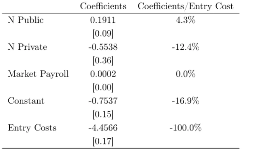
Table 6 reports the structural parameters estimates. Structural parameters are estimated in units of the scale factor in the EV distribution and do not have a level interpretation. Only relative magnitudes matter. To facilitate the interpretation of the coefficients, in the second column of the table we show the coefficient divided by the absolute value of the entry costs estimate. Standard errors of the parameters are calculated by block bootstraping CCPs, logits for the activity decisions of public players and state transitions 50 times. We estimate the structural model 50 times, one for each block bootstrap draw of beliefs and state transitions. We estimate the standard errors for our parameters from the bootstrap sample. A similar procedure has been applied in Ryan (2012) and Collard-Wexler (2013).
The estimated model has also 91 market/bank fixed effects - terms µim in equation (4)33.
For simplicty we do not report these coefficients.
The model predicts that a new private competitor in the market reduces the profit of a private competitor in 12.4% of the entry costs. The entry of a new public bank increases the
32
We tested the robustness of our results increasing the number of periods. The point estimates do not change much when we increase the time horizon.
33
To estimate the model we have 46 different markets whereNpri= 2andNpub = 2. For each market we
profits of a private incumbent in 4.3% of the entry cost. The constant term, which measures operational costs, is negative and relatively larger than competition effects. Entry costs are also negative and large.
Table 6: Structural Parameters for Private Banks, Baseline Model Coefficients Coefficients/Entry Cost
N Public 0.1911 4.3% [0.09]
N Private -0.5538 -12.4% [0.36]
Market Payroll 0.0002 0.0% [0.00]
Constant -0.7537 -16.9% [0.15]
Entry Costs -4.4566 -100.0% [0.17]
Note: Standard-errors in brackets. The standard errors were obtained from 50 block bootstraps of beliefs and transitions. The coefficients are measured in units of standard deviations of the iid profitability shock. The column labeled Coeffs/Entry Costs reports the coefficients as a % of the (absolute value of) entry costs.
6.2
Alternative model
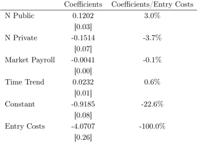
Table 7 reports the estimates for the alternative model. As in the baseline model, parameters are estimated in units of the scale factor in the EV distribution. Standard errors of the parameters were calculated by block bootstraping CCPs and logits for the activity decisions of public players 50 times. As in the baseline model, the alternative model has also 91 market/bank fixed effects. For simplicty we do not report these coefficients.
The first column shows the estimated coefficients; the second shows the coefficients as % of the absolute value of entry costs.
Table 7: Structural Parameters for Private Banks, Alternative Model Coefficients Coefficients/Entry Costs
N Public 0.1202 3.0% [0.03]
N Private -0.1514 -3.7% [0.07]
Market Payroll -0.0041 -0.1% [0.00]
Time Trend 0.0232 0.6% [0.01]
Constant -0.9185 -22.6% [0.08]
Entry Costs -4.0707 -100.0% [0.26]
Note: Standard-errors in brackets. The standard errors were obtained from 50 block bootstraps of beliefs and transitions. The coefficients are measured in units of standard deviations of the iid profitability shock. The column labeled Coeffs/Entry Costs reports the coefficients as a % of the (absolute value of) entry costs.
7
Model Fit and Counterfactual
This section uses the structural model to construct two policy experiments. We are interested in the following questions. First is: what happens with the number of bank branches in small isolated markets when public banks are privatized? Another is: what happens with the number of bank branches in small markets if public banks close down?
To address these questions we solve the model using the estimated parameters. In the baseline model, for each market the solution to the model is a vector of Npri ·Ns entry
probabilities that solves the system of implicit best responses given by equation (7). The alternative model can be solved backwards - see Igami (2014).
For the counterfactual experiment we use only the stationary (baseline) model. A coun-terfactual study using the non stationary model is substantially more complicated34.
34
7.1
Model fit
We begin by solving the system (7) for private banks activity probabilities. To check how the multiplicity affects our conclusions, we proceed in the following way: first, we solve the model for the entry probabilities using the logit probabilities as the initial guess; second, we perturb the logit probabilities; third we compute again the solution for the model using the “perturbed” vector of logit probabilities as the initial guess; fourth, we compare the “perturbed” solution with the original solution35. In doing so we find that the solutions are
identical for any initial guess.
We use the solution for the activity probabilities of private banks, the logit estimates for the activity probability of public banks and the estimated transition process for the municipality payroll to simulate relevant market moments. We compare these moments with the corresponding data moments. For each market in our sample36 we simulate the
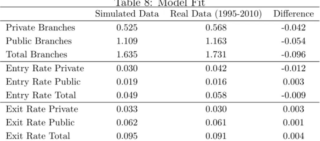
average number of private and public banks, the average number of entry movements of private and public banks and the average number of exit movements of private and public banks from 1995 to 2010. Starting from the state vector of each market in 1995 we simulate 100 paths for these variables 16 periods ahead, until 2010. We compute the average value across paths, years and markets. The next table compares the model’s moments and data moments for the markets in our sample.
Table 8: Model Fit
Simulated Data Real Data (1995-2010) Difference Private Branches 0.525 0.568 -0.042 Public Branches 1.109 1.163 -0.054 Total Branches 1.635 1.731 -0.096 Entry Rate Private 0.030 0.042 -0.012 Entry Rate Public 0.019 0.016 0.003 Entry Rate Total 0.049 0.058 -0.009 Exit Rate Private 0.033 0.030 0.003 Exit Rate Public 0.062 0.061 0.001 Exit Rate Total 0.095 0.091 0.004
Note: Data are simulated taking as initial conditions the state vector in each market in 1995. Real data (1995-2010) has the corresponding moment averaged across markets between 1995-2010.
For private banks, the moments implied by the structural model appear to be quite close
35
Firstly we multiply the original guesses (calculated from the CCPs showed above) by several factors between 0 and 1. We also start the model with a “fixed” guess, where the probabilities for all the states and for all the banks are equal to 0.25, 0.5 and 0.75. We use the same procedure to compute the counterfactuals.
36
to those observed in the data. The model slightly underestimates the average number of private branches across markets/years. This happens because entry rates implied by the model are also slightly underestimated and exit rates are slightly overestimated. Predictions for public banks, which are based on the logit estimates, and the number of public branches predicted by the model are very similar to what we observe in the data.
Next we use this model to construct counterfactuals.
7.2
Counterfactual
This section analyzes the effects of the privatization of public banks on the number of active branches in small isolated markets. The entry decisions of public banks, instead of being generated by an exogenous process, are now calculated according to the system of best responses showed in equation (7). We calculate the equilibrium probabilities for 4 banks. The counterfactual reflects the case where, after privatization, public banks start to operate based on the policy functions of private banks37.
In a second counterfactual experiment we study how the clousure of all public banks would affect the average number of branches in the market. In this experiment we assume that the activity probability of public banks are equal to zero for all possible configurations of the state vector. We solve the system of best responses showed in equation (7) for the 2 private banks imposing this restriction on the behavior of public banks.
In both experiments we assume that payoff parameters are invariant to the policy change. To check how multiplicity affects our conclusions we use the procedure described in Section 7.1. In all experiments the resulting equilibrium did not change38.
Using the counterfactual equilibrium probabilities for each experiment we simulate the average number of private banks, the average number of entry movements of private banks and the average number of exit movements of private banks from 1995 to 2010. Starting
37
We are analyzing municipalities with,ex ante, two public banks and two private banks. After
privatiza-tion we assume that there are four private banks in the market (instead of two public and two private). Two of these players operate based on the behavior (primitives) of one of the pre-existing private banks in that market; the other two operate based on the behavior of the other pre-existing private bank. In other words, in each market, after privatization there are 2 banks with the same profit function (as one of the pre-existing private banks) solving independently problem (5) and 2 private banks with the same profit function (as the other pre-existing private bank) solving independently problem (5). Notice that pre-existing private banks have a different profit function in each market because of the bank/market fixed effect - see equation (4). The equilibrium probabilities under this counterfactual are obtained by solving system (7) for all the four banks and every possible state in each market.
38
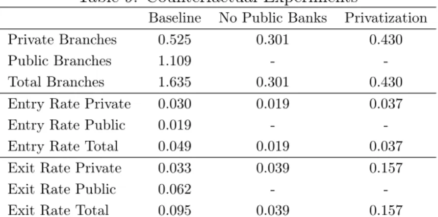
from the state vector of each market in 1995 we simulate 100 paths for these variables 16 periods ahead, until 2010. In Table 9 we show the average of these variables across paths, years and markets for each counterfactual experiment.
Table 9: Counterfactual Experiments
Baseline No Public Banks Privatization Private Branches 0.525 0.301 0.430 Public Branches 1.109 - -Total Branches 1.635 0.301 0.430 Entry Rate Private 0.030 0.019 0.037 Entry Rate Public 0.019 - -Entry Rate Total 0.049 0.019 0.037 Exit Rate Private 0.033 0.039 0.157 Exit Rate Public 0.062 - -Exit Rate Total 0.095 0.039 0.157
Note: Data are simulated taking as initial conditions the state vector in each market in 1995. Real data (1995-2010) has the corresponding moment averaged across markets between 1995-2010.
The first column in the table above is equal to the first column in Table 8. The second column has the corresponding numbers for the world without public banks and the third for the world where public banks are privatized. Without public banks the markets we are analyzing would have on average 0.30 active bank branches per year. If public banks were privatized these markets would have on average 0.43 bank branches per year. In both cases we would observe a significant drop in the number of bank branches in the market.
8
Conclusions
This paper explores microdata of isolated markets in Brazil to estimate a dynamic entry game for public and private banks. We recover banks’ payoffs. The model is solved for the equilibrium entry probabilities. The market equilibrium is evaluated under two counterfac-tual scenarios. In the first counterfaccounterfac-tual public banks are privatized; in the second public banks are closed.
small isolated markets would drop significantly. Under both counterfactual scenarios most of the small isolated markets would end up without any bank branch.
References
[1] Aguirregabiria, V. and P. Mira (2007): “Sequential Estimation of Dynamic Discrete Games”. Econometrica, 75(1), 1-53.
[2] Aguirregabiria, V. and A. Nevo (2010): “Recent Developments in Empirical IO: Dynamic Demand and Dynamic Games”. Advances in Economics and Econo-metrics, Vol. III, Cambridge University Press.
[3] Aguirregabiria, V. and J. Suzuki (2014): “Identification and Counterfactuals in Dynamic Models of Market Entry and Exit”. Quantitative Marketing and Economics, 12(3), 267-304.
[4] Andrade, L. (2007): “Uma Nova Era para os Bancos da América Latina”. The Mckinsey Quarterly, Edição Especial 2007: Criando uma Nova Agenda para a América Latina.
[5] Arcidiacono, P., P. Bayer, J. Blevins, and P. Ellickson (2015): “Estimation of Dynamic Discrete Choice Models in Continuous Time”. Working Paper, Duke University, Department of Economics.
[6] Arcidiacono, P. and R. Miller (2011): “Conditional Choice Probability Esti-mation of Dynamic Discrete Choice Models with Unobserved Heterogeneity”. Econometrica, 79(6), 1823-1867.
[7] Bajari P., L. Benkard and J. Levin (2007): “Estimating Dynamic Models of Imperfect Competition”. Econometrica, 75, 1331-1370.
[8] Bajari, P., H. Hong and D. Nekipelov (2010): “Game Theory and Econometrics: A Survey of Some Recent Research”. Advances in Economics and Econometrics, Vol. III, Cambridge University Press.
[10] Beresteanu, A., P. Ellickson and S. Misra (2010): “The Dynamics of Retail Oligopolies”. Working Paper, University of Rochester, Simon School of Business.
[11] Blundell, R. and S. Bond (1998): “Initial Conditions and Moment Restrictions in Dynamic Panel Data Models”. Journal of Econometrics, 87(1), 115-143.
[12] Bresnahan, T. F. and P. C. Reiss (1991): “Entry and Competition in Concen-trated Markets”. Journal of Political Economy, 99(5), 977-1009.
[13] Burgess, R. and R. Pande (2005): “Do Rural Banks Matter? Evidence from the Indian Social Banking Experiment”. American Economic Review, 95(3), 780-795.
[14] Coelho, C., J. Mello and L. Rezende (2012): “Are Public Banks pro-Competitive? Evidence from Concentrated Local Markets in Brazil”. Forth-coming Journal of Money, Credit and Banking.
[15] Collard-Wexler, A. (2013): “Demand Fluctuations and Plant Turnover in the Ready-Mix Concrete Industry”. Econometrica, 81(3), 1003-1037.
[16] Dunne, T., S. Klimek, M. J. Roberts and Y. D. Xu (2013): “Entry, Exit, and the Determinants of Market Structure”. RAND Journal of Economics, 44(3), 462-487.
[17] Fan, Y. and M. Xiao (2012): “Competition and Subsidies in the Deregulated U.S. Local Telephone Industry”. Working Paper, University of Michigan, De-partment of Economics.
[18] Feler, L. (2012): “State Bank Privatization and Local Economic Activity”. Working Paper, Johns Hopkins University, School of Advanced International Studies.
[19] Gonçalves, L. and A. Sawaya (2007): “Financiando os Consumidores de Baixa Renda na América Latina”. The Mckinsey Quarterly, Edição Especial 2007: Criando uma Nova Agenda para a América Latina.
Critical Access Hospitals”. Eleventh CEPR Conference on Applied Industrial Organization, Toulouse School of Economics.
[21] Gourieroux, C. and A. Monfort (1995): “Statistics and Econometric Models”. Cambridge University Press, Vol. 1.
[22] Gouvea, A. (2007): “Uma História de Sucesso no Setor Bancário da América Latina: Entrevista com Roberto Setúbal, CEO do Banco Itaú”. The Mckinsey Quarterly, Edição Especial 2007: Criando uma Nova Agenda para a América Latina.
[23] Greene, W. (2004): “Fixed Effects and Bias Due to the Incidental Parameters Problem in the Tobit Model”. Econometric Reviews, 23(2), 125-147.
[24] Heckman, J. (1981): “Statistical Models for Discrete Panel Data. Structural Analysis of Discrete Data with Econometric Applications”. Manski, C. and Mc-Fadden D. (eds.). MIT Press: Cambridge.
[25] Hotz, V. J. and R. A. Miller (1993): “Conditional Choice Probabilities and the Estimation of Dynamics Models”. The Review of Economics Studies, 60(3), 497-529.
[26] Hotz, V. J., R. A. Miller, S. Sanders, and J. Smith (1994): “A Simulation Estimator for Dynamic Models of Discrete Choice”. The Review of Economics Studies, 61(2), 265-289.
[27] Igami, M. (2014): “Estimating the Innovator’s Dilemma: Structural Analysis of Creative Destruction in the Hard Disk Drive Industry”. Working Paper, Yale, Deparment of Economics.
[28] Jeziorski, P. (2014): "Estimation of Cost Synergies from Mergers: Application to US Radio". RAND Journal of Economics, 45(4), 816-846.
[29] Kalouptsidi, M. (2014): “Time to Build and Fluctuations in Bulk Shipping”. American Economic Review, 104(2), 564-608.
[31] Levy Yeyati, E., A. Micco and U. Panizza (2007): “A Reappraisal of State-Owned Banks”. Economia, 7 (2), 209-247.
[32] Lin, H. (2011): “Quality Choice and Market Structure: A Dynamic Analysis of Nursing Home Oligopolies”. Working Paper, Indiana University, Kelley School of Business.
[33] Maican, F. and M. Orth (2012): “Store Dynamics, Differentiation and De-terminants of Market Structure”. Working Paper, University of Gothenburg, Department of Economics.
[34] Minamihashi, N. (2012): “Natural Monopoly and Distorted Competition: Evidence from Unbundling Fiber-Optic Networks”. Working paper, Bank of Canada.
[35] Nakane, M. I. and D. B. Weintraub (2005): “Bank Privatization and Produc-tivity: Evidence for Brazil”. Journal of Banking and Finance, 29, 2259-2289.
[36] Nickell, S. (1981): “Biases in Dynamic Models with Fixed Effects”. Economet-rica, 49(6), 1417-1426.
[37] Nishiwaki, M. (2010): “Horizontal Mergers and Divestment Dynamics in a Sun-set Industry”. Working Paper, National Graduate Institute for Policy Studies.
[38] Pascali, L. (2012): “Banks and Development: Jewish Communities in the Ital-ian Renaissance and Current Economic Performance”. Barcelona GSE Working Paper.
[39] Pesendorfer, M. (2010): “Estimation of (Dynamic) Games: A Discussion”. Ad-vances in Economics and Econometrics, Vol. III, Cambridge University Press.
[40] Pesendorfer, M. and P. Schmidt-Dengler (2003): “Identification and Estimation of Dynamic Games”. Working Paper, NBER.
[41] Pesendorfer, M and P. Schmidt-Dengler (2008): “Asymptotic Least Squares Estimators for Dynamic Games”. The Review of Economic Studies, 75 (3), 901-928.
[43] Snider, C. (2009): “Predatory Incentives and Predation Policy: The American Airlines Case”. Working Paper, UCLA, Department of Economics.
[44] Sanches, F. A. M., D. Silva-Junior and S. Srisuma (2015a): “Ordinary Least Squares Estimation for a Dynamic Game”. International Economic Review, forthcoming.
[45] Sanches, F. A. M., D. Silva-Junior and S. Srisuma (2015b): “Identifying Dy-namic Games with Switching Costs”. Working Paper, University of Surrey, De-partment of Economics.
[46] Sweeting, A. (2013): “Dynamic Product Positioning in Differentiated Product Markets: The Effect of Fees for Musical Performance Rights on the Commercial Radio Industry”. Econometrica, 81(5), 1763–1803.
[47] Suzuki, J. (2012): “Land Use Regulation as a Barrier to Entry: Evidence from the Texas Lodging Industry”. International Economic Review 54(2), 495–523.
Appendix 1: Proofs
y(stm;σim,pm) and D(stm;σim,pm) functions. The functions y(st
m;σim,pm) and D(stm;σim,pm) in equation (8) are defined as:
y(stm;σim,pm) =
ln
ln
1
1−Him(ati = 1|stm;σim,pm)
−
βz1 st +1 m |s
t
m;σim,pm
−z0 st +1 m |s
t
m;σim,pm
∆imE˜ξim,
which is a real valued differentiable function that depends only on states, beliefs and tran-sitions and,
D(stm;σim,pm) =
X
at
−im
σim(at−im|stm) ˜Π(atim= 1,at−im,stm)+
βz1 st +1 m |s
t
m;σim,pm
−z0 st +1 m |s
t
m;σim,pm
∆imΠ˜im,
which is a real valued 1×Np differentiable vector that depends only on states, beliefs and
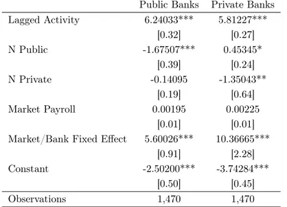
Appendix 2: Logit Estimates, Baseline Model
Table 10: Logits for Activity Decisions of Public and Private Banks Public Banks Private Banks
Lagged Activity 6.24033*** 5.81227*** [0.32] [0.27] N Public -1.67507*** 0.45345*
[0.39] [0.24] N Private -0.14095 -1.35043**
[0.19] [0.64] Market Payroll 0.00195 0.00225
[0.01] [0.01] Market/Bank Fixed Effect 5.60026*** 10.36665***
[0.91] [2.28] Constant -2.50200*** -3.74284***
[0.50] [0.45] Observations 1,470 1,470
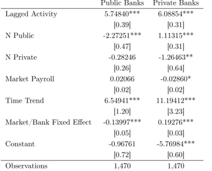
Appendix 3: Logit Estimates, Alternative Model
Table 11: Logits for Activity Decisions of Public and Private Banks Public Banks Private Banks
Lagged Activity 5.74840*** 6.08854*** [0.39] [0.31] N Public -2.27251*** 1.11315***
[0.47] [0.31] N Private -0.28246 -1.26463**
[0.26] [0.64] Market Payroll 0.02066 -0.02860*
[0.02] [0.02] Time Trend 6.54941*** 11.19412***
[1.20] [3.23] Market/Bank Fixed Effect -0.13997*** 0.19276***
[0.05] [0.03] Constant -0.96761 -5.76984***
[0.72] [0.60] Observations 1,470 1,470
![Table 5: Effects of n pub,t− m 1 and n pri,t− m 1 on the Activity Probabilities of Private Banks (GMM) (I) (II) Nº Public 0.02015*** 0.01956*** [0.00] [0.00] Nº Private -0.02856*** -0.01737*** [0.00] [0.00]](https://thumb-eu.123doks.com/thumbv2/123dok_br/16728024.745433/14.892.198.719.180.419/table-effects-activity-probabilities-private-banks-public-private.webp)