ESCOLA DE P ´
OS-GRADUA ¸
C ˜
AO EM
ECONOMIA
William Michon Junior
Essays in Applied Microeconomics
Essays in Applied Microeconomics
Tese para obten¸c˜ao do grau de doutor apre-sentada `a Escola de P´os-Gradua¸c˜ao em Eco-nomia. Data da defesa: 13/07/2015.
´
Area de Concentra¸c˜ao: Teoria Econˆomica
Orientador: Humberto Luiz Ata´ıde Moreira
Michon Junior, William
Essays in Applied Microeconomics / William Michon Junior. – 2015. 93f.
Tese (Doutorado) - Funda¸c˜ao Getulio Vargas, Escola de P´os-Gradua¸c˜ao em Economia.
Orientador: Humberto Luiz Ata´ıde Moreira. Inclui Bibliografia.
1. Microeconomia. 2. Risco (Economia). 3. Petr´oleo - Aspectos econˆomicos. I. Moreira, Humberto Ata´ıde. II. Funda¸c˜ao Getulio Vargas. Escola de P´ os-Gradua¸c˜ao em Economia. III. T´ıtulo.
Resumo
Esta tese ´e composta de trˆes artigos. No primeiro artigo, “Risk Taking in Tournaments”, ´e considerado um torneio dinˆamico no qual jogadores escolhem como alocar seu tempo em atividades que envolvem risco. No segundo artigo, “Unitiza¸c˜ao de Jazidas de Petr´oleo: Uma Aplica¸c˜ao do Modelo de Green e Porter”´e analisado a factibilidade de se haver um acordo de coopera¸c˜ao em um ambiente de common-pool com incerteza nos custos das empresas. No terceiro artigo, “Oilfield Unitization Under Dual Fiscal Regime: The Regulator Role over the Bargaining”, por sua vez, ´e estudado a unitiza¸c˜ao quando existem dois regimes fiscais distintos, como os jogadores se beneficiam disso e o papel do regulador no regime de partilha.
Abstract
This dissertation comprises of three articles. The first article, “Risk Taking in Tourna-ments”, considers a dynamic tournament model where players choose how to spend their time in activities that involve risk. The second article, “Unitiza¸c˜ao de Jazidas de Petr´oleo: Uma Aplica¸c˜ao do Modelo de Green e Porter” analyses the feasibility of a cooperation agreement under a common-pool problem where the production cost is uncertain. The third article, “Oilfield Unitization Under Dual Fiscal Regime: The Regulator Role over the Bargaining”, by its turn, studies the unitization when there exist two different fiscal regimes and how firms are benefited by this distortion, and the role of the regulator in the profit sharing contract.
1.1 Tournament Timing. . . 18
1.5 Equilibrium with x1 = 3 . . . 24
1.6 The Effect of x1 over players’ Strategy . . . 25
1.9 Player A Choice of Expected Output and Volatility. . . 39
1.10 Player B Choice of Expected Output and Volatility. . . 39
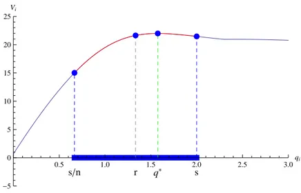
2.1 Fun¸c˜ao Valor V𝑖 . . . 62
2.2 Condi¸c˜ao de Primeira Ordem da firma iquando j ̸=i jogam q⋆ . . . 62
2.3 Condi¸c˜ao de Primeira Ordem da firma iquando j ̸=i jogam s . . . 63
3.1 Optimal production plan . . . 80
3.2 Transfer . . . 83
3.3 π1(q𝑅) −π2(q𝑅) when λ2 = 0.4, for b= 3 and b= 2, respectively. . . . 88
3.4 t𝑅 1 contour plot . . . 89
1 Risk Taking in Tournaments 11
1.1 Introduction . . . 11
1.2 Related Literature . . . 14
1.3 The Static Model . . . 17
1.3.1 Environment . . . 17
1.3.2 Tournaments Incentives . . . 19
1.3.3 Equilibrium . . . 22
1.3.4 Two Periods Tournament Model . . . 26
1.4 The Dynamic Model . . . 28
1.5 Other Extensions for the Static Tournament . . . 35
1.5.1 Asymmetric expected output . . . 36
1.5.2 Tie-Break Rule . . . 37
1.6 Conclusion . . . 40
Bibliography . . . 42
2 Unitiza¸c˜ao de Jazidas de Petr´oleo: Uma Aplica¸c˜ao do Modelo de Green e Porter 43 2.1 Introdu¸c˜ao . . . 43
2.2 O problema dos recursos comuns e a unitiza¸c˜ao . . . 44
2.3 Aplica¸c˜ao do Modelo de Green e Porter . . . 48
2.3.1 Desenho do contrato ´otimo . . . 54
2.3.2 Exemplo com a distribui¸c˜ao de Pareto . . . 60
2.4 Conclus˜ao . . . 63
Referˆencias Bibliogr´aficas . . . 66
Apˆendice A - Condi¸c˜oes de primeira ordem do contrato ´otimo . . . 67
3 Oilfield Unitization Under Dual Fiscal Regime: The Regulator Role over the Bargaining 69 3.1 Introduction . . . 69
3.3 Literature . . . 74
3.4 The Environment . . . 76
3.4.1 The common-pool problem . . . 77
3.5 The Bargaining Problem . . . 78
3.6 Two Models of Negotiation Breakdown . . . 81
3.6.1 Rule of capture resolution . . . 81
3.6.2 Regulator resolution . . . 85
3.6.3 Comparing the solutions by numerical analysis . . . 89
3.7 Conclusion . . . 90
Risk Taking in Tournaments
Abstract
We study a tournament model where players must decide how to allocate their time in different activities, associated with different levels of risk. At first, we describe and study the static version of the model, where there is an optimal choice of variance that induces the highest expected output. Under a piece-rate, this would be the choice of the player, but under tournaments, players deviate from this choice to increase the probability of winning. In the dynamic setting, we show how a player seeks more or less risk as the games comes to the end. Finally, we presents the tie-break rule as a way the principal can improve the expected output.
1.1
Introduction
among the most widespread ways to provide incentives and granting higher salary, bonus and promotions.
The contract theory literature has embraced tournaments as a descriptive model of incentives within firms. Workplace contests are among the most common motivating applications of the theoretical tournament literature. Tournaments among workers can mitigate incentive problems when the effort of workers is unobservable. A key idea un-derlying tournament theory is that there are clear winners and losers, and the rewards are usually indivisible, so the knowledge of it provides the incentives agents need to effort towards firms’ goals, if the mechanism is well set. The incentive comes from the rational-ity of the players who seek to maximize their individual utilrational-ity by increasing the chance of winning a prize. In contrast with other forms of remuneration, such as piece rates – where players are paid according to their production –, tournaments may involve lower information costs. It is generally cheaper to track the relative performance levels rather than to monitor absolute performance levels, especially when it involves few competitors. For example, PhD programs and employers skim through the information available of the applicants, and carefully evaluate only the very top of them. This is especially true when employees are compared in order to be rewarded, since it can isolate the common shocks that might occurred during the evaluation period. The piece rate could provide the wrong compensation for players’ effort, or the employer would need to be informed about the market conditions before cross off the aggregate shock term from their performance. The relative performance evaluation removes the risk of common uncertainty, so it can reduce the amount of money paid to players, since it also work as an insurance. Both players and principal know the maximum and the least amount of money they will spend/earn.
Nevertheless, effort may not be the only choice an agent has while competing in a tournament. In sports, a coach and his team can choose different levels of risk in a game, for example, in a soccer match the team losing the game can switch a defense player for an offensive player to increase the probability of scoring a goal. We can also observe it in other sports, like in a hockey game, when a team switch the goalie for a line player, or in car racing, where the driver can choose risky paths to overcome someone ahead of him. Not only in sports we can observe it, but also in many other situations, like labor market and financial market. An employee can exert risky tasks in order to increase his chance to be promoted, like a loan officer that selects different projects to finance and his reward depends on the return of his loans compare to the other officers. An investment fund that balances its portfolio based on expected return and risk. A CEO can affect the riskiness of the company’s production and profit, based on his choice of research project, the kind of employee he selects and the market he would like to explore, in addition to deciding how hard they will work.
In the investment funds industry, for example, firms face a trade-off between ex-pected return and risk of their portfolio. It is also possible that two different portfolios have the same expected return, but different volatility. There might be an optimal way to balance the portfolio, in terms of expected return adjusted by the risk of it. However, in a tournament players can be encouraged to seek more risk than the one that generates the highest expected return, in order to increase the probability of wining during a dynamic competition. Funds are evaluated periodically, and when it lacks performance relative to other funds, it may have incentives to deviate from the optimal choice of expected return and increase the risk of their portfolio in order to increase its probability of being the top performer and thus receiving larger amount of investment flow. We can also see this the trade-off between risk and expected output in other activities, for example, an advertisement sales, in which salespeople spend their time contacting the usual clients or they can spend time in prospecting new clients.
volatility seeking to increase their probability of winning. Our main goal is to model the dynamic behavior during a tournament. In a dynamic setting, we found that players’ behavior towards risk evolves overtime, and as the game is near the end, players will seek more risk if there are losing, and will avoid risk if they are leading. To the best of our knowledge, this behavior was not modeled yet, though it is a common wisdom.
Next section we will survey the related literature about tournament theory with risk taking. Section1.3we describe the model and compute the equilibrium for the static case. Sections 1.3.4 and 1.4 we describe the tournament with two and T periods, respectively. The Section1.5 we consider the static case again, and discuss the assumption about the symmetric expected output function and what would happen if we relax this assumption. We also present a tie-break rule, so in order to win the prize they must perform much more than their opponent. We show numerically how the principal can improve players’ output by setting correctly the tie-break rule.
1.2
Related Literature
The formal study of this reward structure has started with Lazear and Rosen (1981), in a labor market model. They provide an alternative model to understand why some employees earns much more after a promotion, even though they perform a similar job without increasing his marginal productivity. The idea is that players can be encouraged to effort by competing against their peers for a promotion or wage rise. Their paper shows that tournament schemes can implement first-best levels of effort, when agents are risk neutral and the prizes are carefully chosen.
than they do in the first best solution, but it would require the principal to compensate them in order encourages them to participate in the contest. Furthermore, introducing a tie-break rule, it is possible to improve the tournament solution with respect to the principal outcome.
However, in the real world the effort is not the only possible choice that workers have. Sometimes agents can influence both the spread of distribution of the output and the distribution mean. For example, a loan officer chooses projects with different expected returns and risks, managers can choose innovative or conservative technology strategies and fund managers can choose the riskiness and expected returns of their portfolio. To the best of our knowledge, Bronars (1987) was the first to consider the idea of player manipulating the risk to increase the probability of winning. The first published paper about risk taking in tournament is Hvide (2002), which studies the incentives for risk seeking by the identical players in a symmetric equilibrium. Since the choice of risk is costless in his model, players choose the maximum variance in order to reduce the costly effort they must do to overcome the opponent. Increasing variance in a symmetric case will reduce the incentives to do a costly effort, since the marginal increase in the probability of winning by increasing effort is low. Therefore, when players are identical, this compensation scheme induces a “risky-lazy” equilibrium, where both players choose infinity variance and zero effort.
Two papers that studied the asymmetry of player are Kr¨akel and Sliwka (2004), and Kr¨akel(2008), by considering different players’ abilities. They introduce a two-stage model, where players choose the risk level, which is costless, and then the costly effort. According to them, the choice of variance has two effects: (i) the effort effect, which is the reduction of the importance of the effort due to the larger level of noise in the output, and hence, players can reduce their effort level; and (ii) likelihood effect, which is the change in the probability of winning related to the choice of risk. They show that if the leader has a large enough advantage, he would chose low-risk strategy, while the underdog’s choice depends on the cost of effort. When the cost is high, the underdog will choose high-risk strategy. If the advantage is not so large, the underdog will always choose high-risk strategy, while the leader would choose high-risk strategy when the effort cost is low. Gilpatric (2009) presents a model more closely related to ours, in the sense he introduces a costly choice of risk, and propose a penalty that the last placed player must bear, and thus it reduces the excessive risk taking by players in a tournament and control the productive effort, but he does not explore the dynamic effect of risk taking.
midterm information affects players’ decision in the last period of a two-stage tournament, where the risk choice is not available for the players. Since the output is stochastic, in the beginning of the second period one of the players will have an advantage, and if the information about the advantage is fully disclosed, then both players will have incentives to reduce effort. For the underdog, the marginal gain in the probability of winning is reduced and the cost to exert effort to tie the leader’s advantage is high. However, if the principal does not reveal the information about the advantage, players would be less heterogeneous, and thus they would exert more effort than in the full disclose information tournament.
Cabral (2003) and Anderson and Cabral (2007) are the first to study a dynamic tournament where players’ decision involve choosing the variance of an output. They consider an infinite time horizon, where players receive a payoff for each instant of time depending on their position. The background for their model is the research and develop-ment competition in an oligopolistic industry. Two players choose the volatility of their product quality at each instant, and receive a payoff according to the quality difference. Since the game has no end, players choice depends only on the previous quality difference and their patience. The linearity of their model results in a bang-bang solution, and their findings are that for sufficiently patient player, the underdog (or laggard) chooses high risk, while the leader will choose low-variance strategy.
Genakos and Pagliero (2012) empirically study the impact of interim rank on risk taking using data from weightlifting competitions. In this sport, players must announce the weight they will attempt to lift at the beginning of each stage. The authors consider the relative increase of the announcements as a measure of risk, that is, how much a player increased his announcement from the previous one relative to the player placed first. In order to evaluate the players’ behavior towards the risk, they estimate three different models: (i) Announcement vs Ranking; (ii) Announcement vs Absolute distance from competitors; and (iii) Announcement vs Intensity of the Competition. In the first model, they found an inverted-U relationship between the announcement and interim ranking, that is, the announcements increase from the first to sixth place but then decrease for further decreases in rank. One possible reason for riskier strategies for the third and fourth rank is the prize discontinuity between them, which provides incentives to take risk. In the model (ii), they found the expected relationship between risk taking and distance from competitors. A player choose riskier strategy when the competitor in front is close and the trailing player is far. On the other hand, a player reduces the risk when the competitor in front is far and the one trailing is close. Finally, in the model (iii), they measure the intensity of competition by the number of athletes that are close to each other, and they found that more intense competitions stimulates more risk taking. However,Genakos and Pagliero (2012) did not consider how risk taking by the competitors evolves along the time, since their main concern was to evaluate how ranking affects the risk taking.
Although it is a common wisdom players’ behavior in a dynamic tournament, to the best of our knowledge, no theoretical study has modeled how players seek more or less risk as the game is near the end. The main purpose of this paper is to evaluate players’ behavior in the dynamic tournaments. At first, we will introduce the static model, in which one player has an exogenous advantage at the beginning of the period, and evaluate how players seek risk. In Section 1.4 we present the dynamic model, where players start the tournament at the same position, and thus the advantage becomes endogenous. Next section we describe the basic model in a static setting, where the advantage is exogenous. We show the tournament incentives leads to inefficiency, and show how players behave in the equilibrium.
1.3
The Static Model
1.3.1
Environment
We consider two players (i = A,B) competing for a prize W > 0, which is granted to the player who produces the most, while the other player receives zero payoff. The tour-nament setting has the following timing: First, players learn their initial (dis)advantage, represented byx1 as the initial advantage of player A, and choose their action. The
out-put is realized and the principal gives the prize to the player with highest outout-put, after observing it. The loser does not receive anything.
Figure 1.1: Tournament Timing.
0 1
Principal chooses
W >0 Players learn
x1
Player choose their action to
produceY𝑖
The outputY𝑖 is
realized. PrizeW given to
the player who produces the most.
The production is a stochastic function of how players spend their time. There are two activities that players can engage in order to produce output, denoted byk ∈ {r,s}. Each of them generates the same expected output per unit of time spent on it, given by the strictly increasing and concave function f(·), so it presents a diminishing marginal output and the player could produce more by working in both activities. The activityr
is riskier than activity s, in the sense that the task r volatility per unit of time spent on it is higher than the volatility of task s. Let τ be the amount of time spent on activity
k, the output generated by this task follows a Normal distribution with mean f(τ) and varianceτ σ2
𝑘, i.e. Y𝑘𝑖 ∼N(f(τ),τ σ2𝑘), where σ2𝑟 > σ𝑠2.
Each player hasτunits of time available to allocate in both of activities. Letτ𝑖 be the
amount of time playerispends on the riskier activity,r, thusτ−τ𝑖 is the amount of time
spent on the “safe” task,s. After players learnx1, they choose simultaneously how to spend
their time by choosingτ𝑖
∈[0,τ]. Observe that for each possible time allocation by player
i, the outputY𝑖 generated by a choiceτ𝑖 follows a Normal distribution with meang(τ𝑖 𝑡)≡ f(τ𝑖) +f(τ
−τ𝑖) and variance τ𝑖σ2
𝑟 + (τ −τ𝑖)σ𝑠2. The outputs are independent, since
the random term is independent between players and tasks. Therefore, the total output produce by player i follows a Normal distribution,Y𝑖 ∼N(g(τ𝑖), τ𝑖σ2
𝑟+ (τ −τ𝑖)σ𝑠2))
Note that the variance of the output is basically a convex combination between σ2
𝑠
and σ2
𝑟, where the weights are the time allocated in each activity. The function g is even
with respect to 𝜏/2, i.e. g(τ) = g(τ −τ), and thus we have the following two properties:
equidistant to𝜏/2 has the same magnitude but with different sign, and; (ii)g(·) is strictly
increasing in [0,𝜏/2) and strictly decreasing in (𝜏/2,τ].
We can see that the maximum expected output is attained whenf′(τ𝑖) = f′(τ−τ𝑖),
and since f(·) is strictly increasing, the maximum is achieved when τ𝑖 = 𝜏/
2 = τ −τ𝑖.
The Figure 1.2 shows us the function g, which is equivalent to the set of possible choices a player has.
Figure 1.2: Set of Possible Choices
Since the choice of how the time is allocated allocation is costless, in any payment scheme based on production, one would expected that the player would choose the alloca-tion that maximize the output, i.e.,τ𝑖 =𝜏/
2. However, in a tournament payment scheme,
when a player is in disadvantage he might be willing to increase variance of his output in order to increase the chance of getting a higher output.
1.3.2
Tournaments Incentives
A tournament is a compensation scheme in which contestant’s rewards are based on their ordinal position alone and not on the actual size of their output. This scheme pays
W > 0 to the player with highest output and zero to the second player. Players decide
simultaneously their action, seeking to increase their probability of winning the prize, which depends on player A and B choices and the distribution of the random variables that affects both players output. If we introduce an advantage to player A, denoted by
x1, formally we have,
max
𝜏𝐴 W
P[︀x1+Y𝐴(τ𝐴)> Y𝐵(τ𝐵)]︀ (1PP𝐴)
distri-bution, and rewrite the objective function, using the time constraint as
P[︀x1+Y𝐴(τ𝐴)> Y𝐵(τ𝐵)]︀= Φ (︃
x1+g(τ𝐴)−g(τ𝐵)
√︀
(τ𝐵+τ𝐴)σ2
𝑟 + (2τ −τ𝐵−τ𝐴)σ𝑠2 )︃
,
where Φ is the standard Normal cumulative distribution function. In order to ease the notation, denote
η2 =(︀
τ𝐴+τ𝐵)︀
σ2𝑟+ (2τ−τ𝐴
−τ𝐵)σ2
𝑠
and
z = x1+g(τ
𝐴)
−g(τ𝐵)
η .
In order to see the incentives behind a tournament scheme, we will study the first order condition of the player A, which is the following
0 = W
η φ(z) [︂
f′(τ𝐴)−f′(τ−τ𝐴)− σ
2
𝑟−σ𝑠2
2η z ]︂
⇐⇒ f′(τ𝐴)
−f′(τ−τ𝐴) = σ𝑟2−σ𝑠2
2η z.
(1.1)
As we can see in the above equation, it is not necessarily true that player maximize the expected output, i.e. it’s not always true that f′(τ𝐴)
−f′(τ −τ𝐴) = 0. This would
happen if their contract was based on output production, but since they are working under a relative performance evaluation (RPE) contract, a distortion can happen and the best response for the player will not be to maximize expected output anymore. In a tournament, players want to maximize their probability of winning the prize by allocating their time in two activities. The leader would want to remain with the advantage to win the game, so he is willing to sacrifice some of the expected output in order to reducing the risk. By doing it, the noise effect over leader advantage is reduced. On the other hand, the underdog would be willing to sacrifice some of the expected product he would get by maximizing the output, in order to increase the volatility of his output. Thus, he would be reducing the effect of the disadvantage.
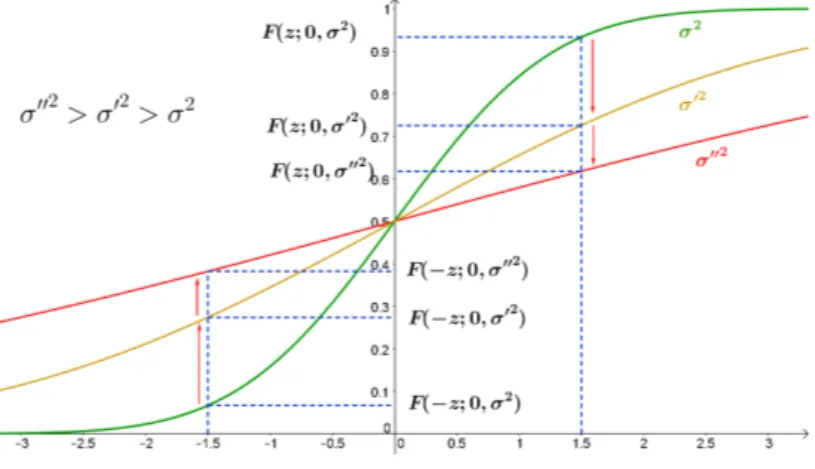
Figure1.3illustrates the general idea about incentives in tournaments, when a player has an advantage towards the other. Suppose player A starts with 1.5 units of output in the beginning of the game, while the other player has no output yet. In this simple example, the figure shows the probability playerAwins when they both decide to produce at the same expected output, but with different levels of risk. In this example, player A
would prefer to reduce his risk, by choosing the variance equals toσ2. On the other hand,
higher risk, so the initial disadvantage has lower influence over the outcome. Figure 1.3: Probability of PlayerA win the Tournament
In the next subsection, we will provide different ways to read the first order condition from (1.1).
Return on Time Allocation
We can rewrite the Equation (1.1) in terms of marginal return of the time allocate to each activity, and we can see the each player equates the marginal return of the risky and safe activity, as shown by the following equation:
f′(τ𝐴)− σ
2
𝑟
2ηz =f ′(τ
−τ𝐴)− σ
2
𝑠
2ηz. (1.2)
This equation shows on l.h.s. the marginal return of allocating an additional fraction of the time on the risky activity, while the r.h.s. the same for safe activity. Note that since
σ2
𝑟 > σ2𝑠, the (dis)advantage affects more the risky choice. The Figure 1.4 illustrates this
equation.
Figure 1.4: Player A first order condition
Notes: To plot this figure, it was used τ𝐵 = 1
2, σ2𝑠 = 1, σ𝑟2 = 2 and
Note that Figure 1.4 is based on the risky activity time allocation, i.e. τ𝐴.
There-fore, this plot can be interpreted as the marginal benefit of the spending time at the risky activity (red line) versus the marginal cost of opportunity to allocate time in this activity (blue line), which is given by the marginal benefit of spending time at the safe activity. First note that they are not symmetric, sinceσ2
𝑟 > σ𝑠2, hence one player will be willing to
deviate from the maximal expected output time allocation, whenever there is a disadvan-tage. If playerA starts with an advantage x1 >0, we will see that z >0, so working an
additional time on the risky task will negatively affect his probability of winning, because
σ2
𝑟 > σ𝑠2. We plotted two possible values forx1, one positive (i.e. playerAhas advantage)
and one negative (i.e. playerB has advantage). We can see that when the playerAhas an advantage, the best response for him is to allocate more time in the safe activityτ𝐴<𝜏/2,
while when he is losing he prefers to work more on risky activities. We can also see that the risky activity is more sensitive with variations onx1, since σ2𝑟 > σ𝑠2.
1.3.3
Equilibrium
In the previous section, we analyzed the best response of a player, and it was shown the effects of the advantage and the variance in this model. Now, we will characterize the Nash equilibrium of this static tournament. From Equation (1.1) we have the best response of player A. For player B, the only change is that the probability of winning is 1−Φ(x), and thus, the system to be solved has the following equations:
f′(τ𝐴)
−f′(τ−τ𝐴) = σ𝑟2−σ𝑠2
2η z and f ′(τ𝐵)
−f′(τ −τ𝐵) =
−σ
2
𝑟 −σ𝑠2
2η z (1.3)
Proposition 1 A pure-strategy equilibrium exists, if the following condition holds:
inf 𝜏𝑖 ⃒ ⃒ ⃒ ⃒
g′′(τ𝑖) g′(τ𝑖) ⃒ ⃒ ⃒ ⃒ > σ 2
𝑟 −σ𝑠2
2τ σ2
𝑠
. (1.4)
The players’ equilibrium choice will satisfy the following equations:
g′(τ𝐴) = σ
2
𝑟−σ𝑠2
2
x1
τ(σ2
𝑟 +σ𝑠2)
and g′(τ𝐵) =−σ
2
𝑟 −σ2𝑠
2
x1
τ(σ2
𝑟 +σ2𝑠)
(1.5)
Proof. Note that Φ is a strictly increasing function, so we are interested in maximizing it’s argument, defined by
z = x1+g(τ
A sufficient condition for a pure-strategy Nash equilibrium to exist is that z strictly concave in playerAchoice given any choice of his opponent. The existence is guarantee if
g′′(τ𝐴)
−η𝜏𝐴𝜏𝐴
g′(τ𝐴) η𝜏𝐴
<0, for all τ𝐴 and τ𝐵,
where η𝜏𝐴 is the partial derivative of η with respect to τ𝐴 and η𝜏𝐴𝜏𝐴 is the second order
partial derivative of η with respect to τ𝐴. This condition holds if g′(τ𝐴) = 0, since g is a concave function. If g′(τ𝐴) < 0, this condition also holds, because η is a strictly
increasing and concave function inη. Wheng′(τ𝐴)>0, a sufficient condition to guarantee
the existence is
inf 𝜏𝐴 ⃒ ⃒ ⃒ ⃒
g′′(τ𝐴) g′(τ𝐴) ⃒ ⃒ ⃒ ⃒
> sup
𝜏𝐴,𝜏𝐵
⃒ ⃒ ⃒ ⃒
η𝜏𝐴𝜏𝐴 η𝜏𝐴 ⃒ ⃒ ⃒ ⃒ .
Since τ𝑖
∈ [0,τ], the right-hand side is equal to (𝜎2
𝑟−𝜎
2
𝑠)/2𝜏 𝜎2
𝑠, thus we have the condition
(1.4). The condition for playerB is the same, but−zneeds to be concave inτ𝐵. Assuming
that (1.4) holds, we can characterize the equilibrium by using the first order condition. We can rewrite the Equation (1.3) using the function g(·) and equalize them, so we find g′(τ𝐴) =
−g′(τ𝐵). But using that g′(τ) = −g′(τ −τ), we rewrite the equilibrium
condition asg′(τ𝐴) = g′(τ−τ𝐵), and since g is strictly concave, we haveτ𝐴=τ
−τ𝐵, or τ𝐴+τ𝐵 =τ.1 We now rewrite η2 =τ(σ2
𝑟 +σ2𝑠) and thus at the equilibrium we have
z = √︀ x1
τ(σ2
𝑟 +σ𝑠2) ,
thus we have the equations (1.5).
This proposition shows how players behave depending on the initial advantage x1.
Ifx1 is positive, it means that playerA is ahead of playerB, and thatg′(τ𝐴)>0, that is,
player A will choose τ𝐴<𝜏/2, so he is allocating more time on the safe activity, in order
to reduce the volatility of his output. On the other hand, ifx1 is negative, so player A is
behind playerB, we will have the opposite behavior, that is, he will seek risky activity in order to increase his output volatility, so he can increase the probability of winning the game.
The idea is that whenever a player has some advantage, ‘his probability of winning the tournament is greater than 1/2. In order to maintain his advantage, he avoids
allo-cating time to risky activity, since it would increase the variance of his output and thus reduce the probability of winning the tournament. On the other side, the player with dis-advantage has the opposite incentive, since he could increase his probability of winning by increasing the output variance. However, if no one has any advantage, then both players
will maximize their expected output.
Figure 1.5 shows the reaction function from both players and the equilibrium when
x1 >0, that is, player A starts with an advantage. The figure is plotted in the following
way: The blue line is the reaction function for playerA, the abscissa contains all possible choices for player B, and the line shows player A best reaction. The red line is the reaction function for playerB, and the ordinate has all possible choices for playerA. The intersection of these two lines is the Nash equilibrium for this static tournament. The yellow dashed line represents the symmetric choices, that is τ𝐴=τ𝐵.
In order to maintain his advantage, playerAwill allocate more time to safe activities, reducing the volatility of his output. On the other hand, player B seeks risky activities so that he reduces the probability of player A wins the tournament, since he will be increasing the variance of his output and of the output difference.
Figure 1.5: Equilibrium with x1 = 3
(a) Reaction functions (b) Equilibrium choices on Mean-Variance Frontier
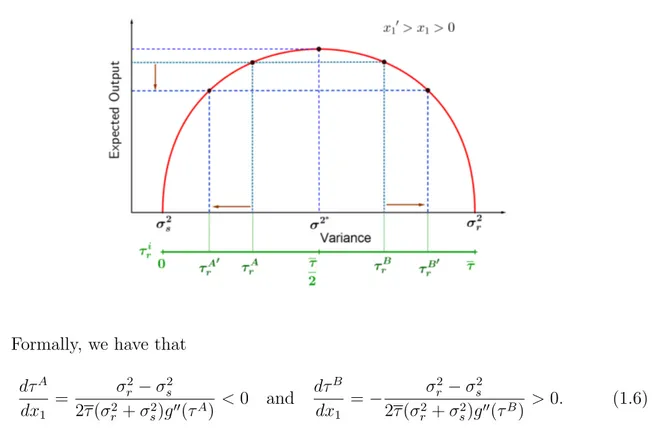
Equation (1.5) shows the behavior of the players towards changes in the parameters of the model. Formally, we can use the implicit differentiation this equation to view the effect of changes in the parameters. First, note that function g is strictly concave, so the derivative of the inverse function of g′ is decreasing. Let us explore this properties
beginning with the advantage effects. As x1 > 0 increases, the player A, who has the
Figure 1.6: The Effect of x1 over players’ Strategy
Formally, we have that
dτ𝐴 dx1
= σ
2
𝑟 −σ𝑠2
2τ(σ2
𝑟+σ𝑠2)g′′(τ𝐴)
<0 and dτ
𝐵
dx1
=− σ
2
𝑟 −σ𝑠2
2τ(σ2
𝑟 +σ𝑠2)g′′(τ𝐵)
>0. (1.6)
The magnitude of the change clearly depends on advantage, but also depends on the time endowment, concavity of the expected output and variance parameters. When the variance associated to the risky activity is relatively large to the safe risk, the player who has an advantage will seek safer tasks even more, since he tries to reduce his output volatility, while the underdog do the opposite. Theg′′ term represents how the marginal
expected output changes at each unit of time allocated on the risk activity. The more negative is g′′, means that a small change on the risk affects more severely the expected
output, so the player who has advantage will avoid reducing too much the risk compared to the optimal choice of𝜏/2, since it would have a large negative impact over his expected
output. Finally, the higher is the endowment of time, τ, since it also affects g′′ in the
opposite way, thus the overall effect is ambiguous.
The variance associated with the risky activity also affects players’ choice, as ex-pected. The higher is the variance of such activity, the less the leader will allocate time on it, since it will reduce his probability of winning. The marginal effect will depend on the advantage, endowment and on the second derivative of g. Again, the higher is the advantage, the more willing the leader will be to reduce the variance of his output, even though losing in terms of expected output. The g′′ term has the same intuition as in the
previous paragraph. The trade-off between allocating time to risk and safe activity now appears in this marginal effect:
dτ𝐴 dσ2
𝑟
= x1
g′′(τ𝐴)
σ2
𝑠 τ(σ2
𝑟+σ𝑠2)2
<0 and dτ
𝐵
dσ2
𝑟
=− x1
g′′(τ𝐵)
σ2
𝑠 τ(σ2
𝑟 +σ𝑠2)2
so, as the variance of the safe activity increases, so the term 𝜎𝑠2 𝜏(𝜎2
𝑟+𝜎2𝑠)2 increases, then
the leader will not reduce the time allocation on risk activity too much compared to the optimal choice 𝐻/2. This happens due to the lower trade-off between allocating time to
the risk and safe activity, measured by the differenceσ2
𝑟 −σ𝑠2.
Finally, we can study how the endowment affects the equilibrium choices. Now, the effect over the leader is clear, increasing the time allocated on risk activity, since the optimal level also increases. However, for the underdog, the effect is not clear. It will depend on his disadvantage and on theg′′.
dτ𝐴
dτ =
f′′(τ−τ𝐴) g′′(τ𝐴) −
σ2
𝑟 −σ𝑠2
2τ2(σ2
𝑟+σ𝑠2) x1
g′′(τ𝐴) >0 and dτ𝐵
dτ =
f′′(τ −τ𝐵) g′′(τ𝐵) +
σ2
𝑟−σ𝑠2
2τ2(σ2
𝑟 +σ2𝑠) x1
g′′(τ𝐵).
(1.8) Therefore, we can see that under a tournament scheme, the asymmetry between players and the possibility to take risk will reduce the total expected output. We can also see that the larger is the advantage of one player, the other will seek more risk.
1.3.4
Two Periods Tournament Model
In the previous section, we studied the equilibrium of a static tournament, when one of the player can have an exogenous initial advantage. In this section, we will consider the two period model, in which all players start at the same level, that is, there will not be any player with an initial advantage, i.e. x0 = 0. The objective of this section is to make
the advantage endogenous in the model, in the sense that the advantage at the second period is the realization of the stochastic output of each agent after each player chose their time allocation on both tasks.
In the tournament we study in this section, the principal grants the prizeW >0 to the player who produce the most, while the other player does not receive anything. This is a typical case of promotion, where W can be seen as the increase of the salary for the promoted player. The output that the principal compares to reward the winner is now the sum of the each stage output. The first period, both players start with no initial output, and then choose how to allocate their time endowment τ of the period. The output is realized at the end of the first period, and players learn their (dis)advantage at the beginning of the second period, so they can choose the risk of their output strategically, just as it was solved in the previous section.
In order to solve this problem, we will find the subgame perfect equilibrium by backward induction. First, we solve the second stage problem for a given initial advantage at the second period, x1. We starting solving the second stage, considering that player
was solved in the Section 1.3.3, so now let us focus on the first stage problem. Player A
will solve the following problem
max
𝜏𝐴
1
WP[︀Y1𝐴(τ1𝐴) +Y2𝐴* >Y𝐵
1 (τ1𝐵) +Y𝐵
*
2
]︀
(2PP𝐴)
where Y𝑖*
2 is the player i output when he plays the equilibrium strategy for the second
period. First, we use the equilibrium conditions to rewrite the output difference in the second stage:
Y2𝐴*−Y2𝐵* =g(τ2𝐴*)−g(τ2𝐵*) +σ𝑟 (︂√︁
τ𝐴*
2 ε
𝐴
2𝑟− √︁
τ𝐵*
2 ε 𝐵 2𝑟 )︂ +σ𝑠 (︂√︁
τ −τ𝐴*
2 ε
𝐴
2𝑠− √︁
τ −τ𝐵*
2 ε 𝐵 2𝑠 )︂ =σ𝑟 (︂√︁
τ𝐴*
2 ε
𝐴
2𝑟− √︁
τ𝐵*
2 ε 𝐵 2𝑟 )︂ +σ𝑠 (︂√︁
τ −τ𝐴*
2 ε
𝐴
2𝑠− √︁
τ−τ𝐵*
2 ε
𝐵
2𝑠 )︂
,
since we know thatg(τ𝐴*
2 ) =g(τ𝐵
*
2 ) by the symmetry of the model, thus the only
impor-tant part to be considered is the realization of random variables. The difference for the first period is similar to the first line of the above equation:
Y1𝐴−Y1𝐵 =g(τ1𝐴)−g(τ1𝐵) +σ𝑟
(︂√︁ τ𝐴
1 ε𝐴1𝑟− √︁
τ𝐵
1 ε𝐵1𝑟 )︂
+σ𝑠 (︂√︁
τ −τ𝐴
1 ε𝐴1𝑠− √︁
τ −τ𝐵
1 ε𝐵1𝑠 )︂
,
using the equations above and thatτ𝐴*
2 +τ𝐵
*
2 =τ from the equilibrium condition shown
in the proof of the Proposition1, we can rewrite the probability in the following way
P[︀Y𝐴
1 (τ
𝐴
1 ) +Y
𝐴*
2 >Y
𝐵
1 (τ
𝐵
1 ) +Y
𝐵*
2
]︀
= Φ
(︃
g(τ𝐴
1 )−g(τ1𝐵)
√︀ σ2
𝑟(τ+τ1𝐵+τ1𝐴) +σ𝑠2(3τ−τ1𝐵−τ−τ1𝐴)
)︃
.
Now, let us define z1 and η12:
η12 =σ2𝑟 (︀
τ+τ𝐵
1 +τ1𝐴
)︀
+σ2𝑠 (︀
3τ−τ𝐵
1 −τ1𝐴
)︀
and
z1 =
g(τ𝐴
1 )−g(τ1𝐵)
η1
Clearly, substituting these equation in the player A’s problem, it is easy to see that it is similar to the static problem, whenx0 = 0. So, using the proposition1we know that
players will maximize their output, by allocating their time equally on both activities, i.e., each player will spendτ𝑖
1𝑟 =𝜏/2units of time on each task. Therefore, we can see that
1.4
The Dynamic Model
A natural extension to the previous section is when the tournament hasT periods. Now, we will consider a dynamic tournament, in which both players start with the same output level as before. However, as the tournament develops, a player finds out he is ahead of the other and take strategical actions to increases his chances of winning the tournament at each period. The setting is quite similar as the previous one, but now players will be evaluated afterT periods, and at the end of each period players will learn their position. Here, the principal compares the sum of the output over theT periods, and the prize will be given to the player with the highest output level at the end of periodT.
We consider a T−period dynamic stochastic game with two players (i = A,B), where each of them chooses how to spend their time at each period in order to produce the output Y𝑖
𝑡. The sum of the output over time will be considered by the principal to
determine the winner, who will be granted a prize W > 0, while the loser gets nothing. Let ∆Y𝑡 = Y𝐴
𝑡 −Y𝑡𝐵 be the output difference with respect to player A at period t, then
the principal will grant the prize to player A if x𝑇 ≡ ∑︀𝑇
𝑡=0∆Y𝑡 >0, otherwise player B
will receive the prize. Formally, the last period payoff is a functionu𝑖
𝑇 :X −→R, where X ≡R is the state space of the game and
u𝐴𝑇(x𝑇) = ⎧ ⎪ ⎪ ⎪ ⎨ ⎪ ⎪ ⎪ ⎩
W ,if x𝑇 >0;
𝑊/2 ,if x𝑇 = 0;
0 ,otherwise,
and u𝐵𝑇(x𝑇) = ⎧ ⎪ ⎪ ⎪ ⎨ ⎪ ⎪ ⎪ ⎩
W ,if x𝑇 <0;
𝑊/2 ,if x𝑇 = 0;
0 ,otherwise,
(1.9)
or, as it will be more convenient for computation later,u𝐴
𝑇(x𝑇) =W✶{𝑥𝑇>0}, where✶{𝑥𝑇>0}
is the indicator function that equals 1 when x𝑇 > 0. The utility for player B is similar, except that the prize is given when x𝑇 < 0. The tournament studied here does not consider a midterm reward, so the utility function per period t < T equals zero.
Players make their choice after learning the accumulated output difference x𝑡 ≡ ∑︀𝑡
𝑙=0∆Y𝑙 from the end of previous period, that is, the accumulated output difference up
to the beginning of periodt. We assume that at the initial period both players begin the tournament with no output, thus x0 = 0. We can rewrite the law of motion as
x𝑡+1 =x𝑡+Y𝑡𝐴−Y 𝐵
𝑡 , (1.10)
where the state of the next period x𝑡+1 depends on the current initial state x𝑡 and the
players outputY𝑖
𝑡 realization at the end of the period, after players made their decision.
At each period, players can engage in two activities, denoted byk ∈ {r,s}, to produce the outputY𝑖
in the model from Section 1.3, for each unit of time τ spent on an activity, the expected output will bef(τ), where f(·) is a strictly increasing and concave function, thus having the same property as before, diminishing marginal productivity. Also, by working in a taskk, the player will be subject to output volatility associated with that task, which is given by σ2
𝑘τ, where σ𝑟2 > σ𝑠2. Therefore, given that the player chooses to spend τ units
of time on activityk, the output generated by it follows a Normal distribution with mean
f(τ) and varianceτ σ2
𝑘, that is, Y𝑘𝑡𝑖 ∼N(f(τ),τ σ𝑘2).
Both players have τ units of time available to work in both of tasks. Denote τ𝑖 𝑡 ∈
[0,τ]≡D𝑖be the amount of time playerispend on the riskier activity,r, thusτ−τ𝑖 𝑡 is the
amount of time spent on the “safe” task,s. Due to the diminishing marginal productivity, players will probably work on both activities, and thus the playeri production Y𝑖
𝑡 at the
periodt follows a Normal distribution with mean g(τ𝑖
𝑡)≡f(τ𝑡𝑖) +f(τ−τ𝑡𝑖) and variance τ𝑖
𝑡σ𝑟2+ (τ−τ𝑡𝑖)σ2𝑠, i.e. Y𝑡𝑖 ∼N(g(τ𝑡𝑖),τ𝑡𝑖σ𝑟2+ (τ−τ𝑡𝑖)σ2𝑠), since it is the sum of independent
Normal distributions. Again, we assume the players’ output is independently distributed, hence we can find the transition probabilityq:X×D−→ 𝒫(X), that is the probability density of next period be the state x′ given the current players’ choice and state x, i.e. q(x′;τ𝐴,τ𝐵,x), where 𝒫(X) is the set of probability distributions on the set X. The
transition function can be found by using the properties from Normal distributions, hence we have
x𝑡+1 ∼ N
(︀
x𝑡+g(τ𝐴
𝑡 )−g(τ 𝐵 𝑡 ), σ
2
𝑟 (︀
τ𝐴 𝑡 +τ
𝐵 𝑡 ) +σ
2
𝑠 (︀
2τ −τ𝐴 𝑡 −τ
𝐵 𝑡
)︀)︀
, (1.11)
therefore, q is the probability density function (pdf) of a Normal distribution given by (1.11) and we denote Qas its cumulative density function (cdf).
Formally, the game is a tuple [X,(D𝑖,u𝑖
𝑇)𝑖=𝐴,𝐵,Q]
𝑇
𝑡=0, where X = R for all t is the
state space, D𝑖 = [0,τ] fori=A,B is the action space, that is, the players’ endowment of
time and Q:X×D𝐴
×D𝐵
→[0,1] is the cumulative distribution of the state transition function from x𝑡 tox𝑡+1 given a choice (τ𝐴,τ𝐵).
Therefore, the game proceeds as follows. At period t = 0, both players learn that they are starting the game with no initial output, that is, the initial state isx0 = 0. After
observing the initial state, players choose how to spend their time endowment of τ over the two tasks,τ0 =
(︀ τ𝐴
0 ,τ0𝐵
)︀
, simultaneously and independently from each other. After the realization of both outputs, the statex0 transits to state x1 according to the distribution
mentioned above, that follows the Normal distribution N(x0 +g(τ0𝐴)−g(τ0𝐵),σ𝑟2(τ0𝐴+
τ𝐵
0 ) +σ2𝑠(2τ−τ0𝐴−τ0𝐵)). In the next round, at periodt = 1, after observing the statex1,
players choose how to allocate their timeτ1, and after the realization of the outputs, the
observingx𝑇, and grant the prize W to player A if x𝑇 >0, otherwise player B wins the prizeW.
The nature of the tournament, that is the compensation scheme depending only on the x𝑇, makes different histories of the game lead to a same states, which is the variable observed by the players. This property allow us to focus our attention toMarkov strategies. Letξ𝑖
𝑡 :X →D𝑖 denote the Markov strategy for period t, andξ𝑖 𝑡
≡ {ξ𝑖 𝑙}
𝑡 𝑙=0 the
strategy up to periodt. The complete strategy for the tournament for player iis denoted byξ𝑖 ≡ξ𝑖𝑇
. Now, we can write the expected payoff function based on the strategy profile
ξ≡(︀
ξ𝐴,ξ𝐵)︀
, given by
U(ξ)≡E𝜉[︀u𝑖𝑇 (x𝑇)]︀, (1.12)
where E𝜉 is the expectation taken with respect to the measure induced by transition
probability q(·) and the strategy profile ξ. The equilibrium concept we use to solve the game is the Markov perfect equilibrium (MPE), which considers that players condition their actions only on the current state of the game ξ𝑡. A strategy profile is a Markov perfect equilibrium, if the strategy profile is a subgame perfect Nash equilibrium and the strategies is Markovian. Since we consider a finite horizon game, using the one-shot deviation principle, we can find the equilibrium by backward induction, so we have the following definition.
Definition 1 A (nonstationary) Markov perfect equilibrium (MPE) in this setting is a pair of a finite sequence of value function {V𝐴
𝑡 ,V𝑡𝐵}𝑇𝑡=0 and a Markov strategy profile ξ
such that
❼ The system of Bellman equation
V𝑇𝑖−1(x𝑇−1)≡max
𝜏𝑖 𝑇−1
∫︁
u𝑖𝑇(x𝑇)q(x𝑇|x𝑇−1,τ𝑇𝑖−1,ξ−
𝑖
𝑇−1)dx𝑇 (1.13)
V𝑡𝑖(x𝑡)≡max 𝜏𝑖
𝑡
∫︁
V𝑡𝑖+1(x𝑡+1)q(x𝑡+1|x𝑡,τ𝑡𝑖,ξ− 𝑖
𝑡 )dx𝑡+1 (1.14)
is satisfied for i= A,B, with the expectation induced by the probability distribution q.
❼ The strategy of players are optimal each period t:
ξ𝑖
𝑇−1 ∈arg max
𝜏𝑖 𝑇−1
∫︁ u𝑖
𝑇(x𝑇)q(x𝑇|x𝑇−1,τ 𝑖
𝑇−1,ξ𝑇−−𝑖1)dx𝑇
ξ𝑡𝑖 ∈arg max 𝜏𝑖
𝑡
∫︁
V𝑡𝑖(x𝑡+1)q(x𝑡+1|x𝑡,τ𝑡𝑖,ξ− 𝑖 𝑡 )dx𝑡+1
players’ action, T −1, and for each possible state x𝑇−1 we calculate the timeT −1 value
functions and strategies. Next, we move backward one period to timeT −2, the expected value function considers that players will behave according to the strategy found at the period T −1 in the future, and solve the players’ problem considering the probability induced by the next period strategies and the decision at the periodT −2. We continue the backward induction recursively for the periods T −3,T −4,... until we reach time periodt= 0, and thus we have the equilibrium strategy profile ξ.
Proposition 2 There is a unique interior Markov perfect equilibrium, in which the strat-egy profile ξ is such that ξ𝑖
𝑡 satisfies at each period t the following equation
g′(ξ𝐴𝑡 ) = σ2
𝑟 −σ2𝑠
2
x𝑡
(T −t)τ(σ2
𝑟 +σ𝑠2)
and g′(ξ𝑡𝐵) =−g′(ξ 𝐴
𝑡 ), (1.15) and the value function for each period t is given by
V𝑡𝐴(x𝑡) = WΦ (︂
x𝑡
(T −t)τ(σ2
𝑟 +σ2𝑠) )︂
and V𝑡𝐵(x𝑡) =W [︂
1−Φ
(︂
x𝑡
(T −t)τ(σ2
𝑟 +σ𝑠2) )︂]︂
,
(1.16)
if the following condition holds:
inf 𝜏𝑖 ⃒ ⃒ ⃒ ⃒
g′′(τ𝑖) g′(τ𝑖) ⃒ ⃒ ⃒ ⃒ > σ 2
𝑟 −σ𝑠2
2τ σ2
𝑠
. (1.17)
Proof. At the last period of players’ decision, T − 1, the problem is similar to the one presented in Section 1.3.1. Players learn x𝑇−1 and must choose how to spend their
time in order to maximize their probability of winning the tournament, which depends on the law of motion and the transition distribution. Using the law of motion given by
x𝑇 = x𝑇−1+Y𝑇𝐴−1−Y𝑇𝐵−1, and the Normal distribution of the outputs, the distribution
of x𝑇 will be a Normal distribution with mean x𝑇−1 +g(τ𝑇𝐴−1)−g(τ𝑇𝐵−1) and variance
η2
𝑇−1 =σ𝑟2 (︀
τ𝐴
𝑇−1+τ𝑇𝐵−1
)︀
+σ2
𝑠 (︀
2τ −τ𝐴
𝑇−1−τ𝑇𝐵−1
)︀
. The objective function from Equation (1.13) for playerA can be rewritten as
∫︁ u𝐴
𝑇(x𝑇)q(x𝑇|x𝑇−1,τ𝑇𝐴−1,τ𝑇𝐵−1)dx𝑇 =
∫︁
W✶{𝑥𝑇>0}
1
η𝑇−1
φ (︂x𝑇
−x𝑇−1−g(τ𝑇𝐴−1) +g(τ𝑇𝐵−1)
η𝑇−1
)︂ dx𝑇 =W ∫︁ +∞ 0 1
η𝑇−1
φ (︂
x𝑇 −x𝑇−1−g(τ𝑇𝐴−1) +g(τ𝑇𝐵−1)
η𝑇−1
)︂ dx𝑇
=WΦ
(︂x𝑇
−1+g(τ𝑇𝐴−1)−g(τ𝑇𝐵−1)
η𝑇−1
)︂ ,
the same. Therefore, the Proposition1solves the problem to find the strategy profile for periodT −1:
g′(ξ𝑇𝐴−1) =
σ2
𝑟−σ𝑠2
2
x𝑇−1
τ(σ2
𝑟 +σ𝑠2)
and g′(ξ𝑇𝐵−1) =−g′(ξ
𝐴
𝑇−1). (1.18)
Due to symmetry of the production function of the activities,rands,g′(ξ𝐵
𝑇−1) =−g′(ξ𝑇𝐴−1)
implies that both players will choose an allocation that generates the same expected output, g(ξ𝐵
𝑇−1) = g(ξ𝑇𝐴−1), but different levels of risk such that ξ𝑇𝐴−1 +ξ𝑇𝐵−1 = τ, so
η2
𝑇−1 =τ(σ𝑟2+σ𝑠2). Using this information, we now can find a closed-form solution for the
last period expected value function,
V𝑇𝐴−1(x𝑇−1) =WΦ
(︂
x𝑇−1
τ(σ2
𝑟 +σ2𝑠) )︂
and V𝑇𝐵−1(x𝑇−1) =W
[︂
1−Φ
(︂
x𝑇−1
τ(σ2
𝑟+σ𝑠2) )︂]︂
.
We use the guess-and-verify method to find the value function for the period t. In order to find an educated guess, we can compute the probability of winning by each player, when they play the same strategy of the periodT −1, but taking into account that there will be T −t random variables realizing until the end of the game. So, let the following function be our guess for the playerA’s value function for periodt,
V𝑡𝐴(x𝑡) = WΦ (︃
x𝑡 √︀
(σ2
𝑟 +σ𝑠2)τ(T −t) )︃
and V𝑡𝐵(x𝑡) =W [︃
1−Φ
(︃
x𝑡 √︀
(σ2
𝑟 +σ𝑠2)τ(T −t) )︃]︃
.
(1.19) We will solve the problem for player A, since the player B problem can be done by the same way. In order to verify the guess for the value function, we move forward in the time, so we haveV𝐴
𝑡+1(x𝑡+1) and substituting it in the Equation (1.14), we can solve player
A’s problem. First, letη*2
𝑡 = (σ𝑟2+σ𝑠2)τ(T −t−1), we can rewrite the integral using our
guess as ∫︁ Φ (︂ x𝑡+1 η* 𝑡+1 )︂ 1 η𝑡φ (︂
x𝑡+1−x𝑡−g(τ𝑡𝐴) +g(τ𝑡𝐵) η𝑡
)︂
dx𝑡+1 =
∫︁
F𝑊1(w1)f𝑊2(w1−m)dw1,
whereF𝑊1 is a cdf of a Normal distribution with mean 0 and varianceη
*2
𝑡 , the functionf𝑊2 is a pdf of a Normal distribution with mean 0 and varianceη2
𝑡, andm =x𝑡+g(τ𝑡𝐴)−g(τ𝑡𝐵).
Integrating by parts, we can rewrite it as
Λ(m) =
∫︁
f𝑊1(w1) [1−F𝑊2(w1−m)]dw1.
Differentiating it with respect to x𝑡, we find Λ′(m) = ∫︀
a Normal distribution with mean zero and variance given by the sum of both variances, and hence
Λ(︀
x𝑡+g(τ𝐴
𝑡 )−g(τ 𝐵 𝑡 )
)︀
= Φ
(︃
x𝑡+g(τ𝐴
𝑡 )−g(τ𝑡𝐵) √︀
σ2
𝑟[τ𝑡𝐴+τ𝑡𝐵+τ(T −t−1)] +σ𝑠2[2τ −τ𝑡𝐴−τ𝑡𝐵+τ(T −t−1)] )︃
.
Now we can compute the Nash equilibrium for the period t using our guess, where players solve the following problems
max
𝜏𝐴 𝑡
WΦ
(︃
x𝑡+g(τ𝐴
𝑡 )−g(τ𝑡𝐵) √︀
σ2
𝑟[τ𝑡𝐴+τ𝑡𝐵+τ(T −t−1)] +σ𝑠2[2τ −τ𝑡𝐴−τ𝑡𝐵+τ(T −t−1)] )︃ max 𝜏𝐵 𝑡 W [︃
1−Φ
(︃
x𝑡+g(τ𝐴
𝑡 )−g(τ𝑡𝐵) √︀
σ2
𝑟[τ𝑡𝐴+τ𝑡𝐵+τ(T −t−1)] +σ𝑠2[2τ −τ𝑡𝐴−τ𝑡𝐵+τ(T −t−1)] )︃]︃
.
The solution of these problem can be found by the same way we use in the Propo-sition1, and thus must satisfies the following conditions
g′(τ𝑡𝐴) = σ2
𝑟 −σ𝑠2
2
x𝑡
(T −t)τ(σ2
𝑟 +σ2𝑠)
and g′(τ𝑡𝐵) = −g′(τ 𝐴
𝑡 ), (1.20)
where again we haveg(τ𝐴
𝑡 ) = g(τ𝑡𝐵) andτ𝑡𝐴+τ𝑡𝐵 =τ. Finally, using these conditions, we
can check that our guess (1.19) for the value function is indeed the correct value function:
V𝐴
𝑡 (x𝑡) = WΦ (︃
x𝑡 √︀
(σ2
𝑟 +σ𝑠2)τ(T −t) )︃
and V𝐵
𝑡 (x𝑡) = W [︃
1−Φ
(︃
x𝑡 √︀
(σ2
𝑟 +σ𝑠2)τ(T −t) )︃]︃
.
Thus, by the procedure of guess-and-verify, we found the value function and the strategy profile for periodt. The sufficient condition for uniqueness can be found by the same way as in Proposition 1, which concludes the demonstration.
The strategy profile for periodt is similar to the static equilibrium, except that now it depends on the accumulated output difference up to periodt, and there is a new term,
T −t , which is how many periods have left until the end of the game. This term allow us to formalize the idea about how player behave over a multi-stage tournament.
This idea is formalized in the following corollary.
Corollary 2 Players with (dis)advantage will seek (more) less risk as the game comes to the end.
Proof. Suppose playerA has some advantage, i.e. x𝑡>0. By the implicit differentiation, we have
dτ𝐴 𝑡
d(T −t+ 1) =−
σ2
𝑟 −σ2𝑠
2τ2(T −t)2(σ2
𝑟 +σ𝑠2) x𝑡 g′′(τ𝐴
and
dτ𝐵 𝑡 d(T −t) =
σ2
𝑟−σ𝑠2
2τ2(T −t)2(σ2
𝑟 +σ2𝑠) x𝑡 g′′(τ𝐵
𝑡 ) <0,
where the inequality signs come from the fact that g(·) is a strictly concave function. This corollary shows us how the player behave along the tournament. In words, given an advantage for player A, if the tournament is just beginning and it will endure for a long time, the term on denominator T − t will be higher, reducing the value of
x𝑡. The intuition is that, if the tournament will continue for a long time, there will be higher “uncertainty” about the outcome at the end of the tournament, and thus trying to reduce the variance of the periodtoutcome won’t have much impact at the final outcome. Therefore, players prefer to maximize their output on the early stages of the game. As the game come to the end, the player with advantage will try to secure his position by reducing the time allocate on the risky activity, as now it will have greater impact on the final output. On the other hand, the underdog will seek risk.
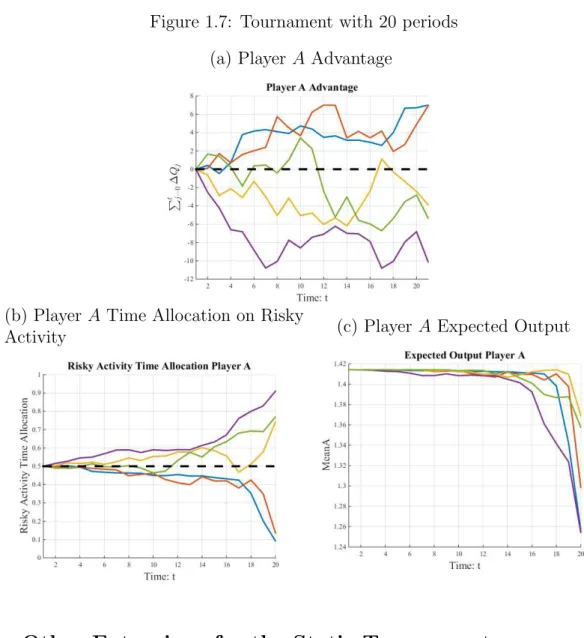
In order to provide an examples and see how player behave over time in a dynamic tournament, we made a simulation of a twenty-period tournament which is shown in Figure 1.7. There are five different realizations of the random variables involved in the tournament, each represented by different color. Each color is a new tournament starting from zero. We show three different figures, where the first is the accumulated output difference, that is, x𝑡, which is the state of the game at the beginning of period t. When the lines are above zero, it means playerA is ahead, and player B is losing. For example, reading figure1.7a, the blue line represents a tournament realization. Both players starts at 0, so there is no advantage at the first period. By the period 5, playerAhas 4 units of output more than playerB. At the end of the tournament, represented by periodt = 21, we can see who was the winner. The dark blue tournament, playerA won approximately by 6.8 output units more than playerB. The light blue line, playerB won the tournament by 10 units more than playerA.
In the Figure 1.7b is depicted how player allocate their time on risk activity. As it was shown by proposition 1, since players start without any advantage, both players chose 𝜏/2, and thus maximize their expected output. As the tournament evolves, some
player will obtain some advantage, and they start to deviate from the optimal choice,𝜏/2.
We can see the proposition 1 working here. Take the dark blue line for example. From the Figure 1.7a, we know that player A is always ahead of player B, so he reduces the volatility of his output by allocating more time to safe activities, i.e. τ𝐴
𝑡 <𝜏/2.
The Figure 1.7c represents the expected output for player A. We can see that he avoids to deviate from the optimal choice 𝜏/2 during most part of the tournament, which
We can also see the proposition2working here, using this three figures. Consider the tournament represented by the light blue line. We can see player A with a disadvantage equal to 10 in 5 different moments (t ≈ 7,8,15,18,20). In Figure 1.7b we can see player
A time allocation on risky activity. By looking at the periods mentioned above, we can see that as the tournament nears the end, he seeks more risk, although he has the same disadvantage at those moments. By the end of the game, he allocates more than 90% of his time on the risky activity. Figure1.7cshows that players avoid distortions on expected output during most part of the tournament.
Figure 1.7: Tournament with 20 periods (a) Player A Advantage
(b) PlayerA Time Allocation on Risky
Activity (c) PlayerA Expected Output
1.5
Other Extensions for the Static Tournament
1.5.1
Asymmetric expected output
We shall discuss the implications of the symmetry of the expected output functionf(·) and what would happen if we relax this assumption. The symmetry of the expected output function helped us to find a closed-form solution for both the static and, especially, the dynamic tournament. The symmetry implies that the function g is even with respect to
𝜏/2, i.e. g(τ) = g(τ −τ), and so the inclination of g for two different points equidistant
to𝜏/2 has the same magnitude but with different sign, i.e. g′(τ) = g′(τ −τ). Therefore,
the equilibrium condition that g′(τ𝐴) =
−g′(τ𝐵) implies that g(τ𝐴) = g(τ𝐵). Another
implication that follows from the function g is even with respect to 𝜏/2 is that we can
write g′(τ) =−g′(τ −τ), and using the assumption that g is a concave function, then g′
will be monotone, and so the equilibrium condition implies that τ𝐴 =τ −τ𝐵. By doing
it, we were able to find a closed form for the varianceη2 and solve the players’ problem.
We can relax this assumption by considering that each activity has a different ex-pected output, sayf𝑟(·) and f𝑠(·). Now, for each τ𝑘 unit time spent on task k by player
i, the output generated by it follows a Normal distribution, i.e. Y𝑖
𝑘 ∼ N(f𝑘(τ𝑘),τ𝑘σ𝑘2).
Denote now the expected total output by playeri as g(τ𝑖
𝑟) = f𝑟(τ𝑟𝑖) +f𝑠(τ −τ𝑘𝑖).
The first order condition would be similar to the Equation (1.3), but now considering two different function for the expected output,
f𝑟′(τ 𝐴
)−f𝑠′(τ−τ 𝐴
) = σ
2
𝑟 −σ𝑠2
2η z and f ′ 𝑟(τ
𝐵
)−f𝑠′(τ−τ 𝐵
) =−σ
2
𝑟 −σ2𝑠
2η z, (1.21)
and again the condition for the equilibrium is
g′(τ𝐴) = σ2𝑟 −σ𝑠2
2η z =−g ′(τ𝐵).
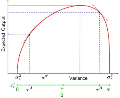
However, since the expected output functions are not symmetric, we cannot find a closed-form solution to the problem as before, and thus we would not be able to use the guess-and-verify method to find the equilibrium in the dynamic model. The Figure 1.8 below illustrates a situation in whichf′
𝑟/f𝑠′ is an increasing function of τ, that is, the marginal
rate of technical substitution is increasing. So, in order to maintain the same level of expected output, reducing one unit of time allocated to risky activity, a player needs to increase in less than one unit of time allocated to the safe activity. We illustrate numerically the case where x1 >0, that is, playerA has an advantage. In this situation,
it becomes harder to determine analytically the signal ofz, that is, if x1+g(τ𝐴)−g(τ𝐵)
Figure 1.8: Set of possible choices of the asymmetric model
1.5.2
Tie-Break Rule
Now, we consider the static model presented in section1.3.1 again, but we will introduce a tie-break rule, in the sense that, if the output of a player are not sufficiently greater than his opponent’ output, the principal will declare a tie. The motivation of this section is to provide further insights about tournaments when the precision of the measure to decide who will be the winner is not good enough. For example, in the swimming competition and car racing, it is possible to determine the winner no matter how close they are, using precision timing of milliseconds. However, in the fund industry, a small difference over performance may not be enough for a fund receive more deposits than the other one. Maybe the investor prefer to move their money to other funds only if they are sufficiently better than the one where the money is deposited due to transaction costs.
In order to do that, let us introduce the tie-break as δ > 0 and now we will need three prizes. To ease the computation, we will consider a symmetric prizes: W,0 and−W, that is, the winner receivesW, if there is a tie both players receive nothing, and the loser must pay W. So, for example, player A wins the tournament, if his output overcomes player B output plus δ, i.e. Y𝐴 > Y𝐵 +δ. This setting could be thought as the case of
investment funds inflow. The winner fund is the one with sufficiently higher performance and will receive an inflow ofW deposit, while the loser will notice an outflow of W from their deposits. However, if the performance of one fund was not sufficiently better, there will be no transfers.