Study of some strategies for disposal of the gnss satellites

(1)

Research Article

Study of Some Strategies for Disposal of the GNSS Satellites

Diogo Merguizo Sanchez,

1

Tadashi Yokoyama,

2

and Antonio Fernando Bertachini de Almeida Prado

1 1_{Instituto Nacional de Pesquisas Espaciais (INPE), 1758 Avenida dos Astronautas,}

12227-010 S˜ao Jos´e dos Campos, SP, Brazil

2_{Universidade Estadual Paulista (UNESP), 1515 Avenida 24A, Caixa Postal 178, 13500-970 Rio Claro, SP, Brazil}

Correspondence should be addressed to Diogo Merguizo Sanchez; diogo.sanchez@inpe.br

Received 3 June 2014; Accepted 15 August 2014

Academic Editor: Chaudry M. Khalique

Copyright © 2015 Diogo Merguizo Sanchez et al. his is an open access article distributed under the Creative Commons Attribution License, which permits unrestricted use, distribution, and reproduction in any medium, provided the original work is properly cited.

he complexity of the GNSS and the several types of satellites in the MEO region turns the creation of a deinitive strategy to dispose the satellites of this system into a hard task. Each constellation of the system adopts its own disposal strategy; for example, in the American GPS, the disposal strategy consists in changing the altitude of the nonoperational satellites to 500 km above or below their nominal orbits. In this work, we propose simple but eicient techniques to discard satellites of the GNSS by exploiting Hohmann type maneuvers combined with the use of the2�̇+ ̇Ω≈0_{resonance to increase its orbital eccentricity, thus promoting}

atmospheric reentry. he results are shown in terms of the increment of velocity required to transfer the satellites to the new orbits. Some comparisons with direct disposal maneuvers (Hohmann type) are also presented. We use the exact equations of motion, considering the perturbations of the Sun, the Moon, and the solar radiation pressure. he geopotential model was considered up to order and degree eight. We showed the quantitative inluence of the sun and the moon on the orbit of these satellites by using the method of the integral of the forces over the time.

1. Introduction

Global navigation satellite systems are a general denomina-tion for constelladenomina-tions of navigadenomina-tion satellites, such as GPS (USA), GLONASS (Russia), Galileo (Europe), and Beidou (China), mainly placed in the medium earth orbit (MEO) region. Up to July 2013, the GPS had 31 active satellites in orbits with altitude near 20,000 km and 55 degrees of inclination. he Galileo system, at the same epoch, had four active satellites, with approximately 23,000 km of altitude and nominal inclination of 56 degrees. he Beidou system is composed by satellites in MEO, geosynchronous orbit (GEO), near circular, and inclined (55 degrees) geosynchronous orbit (IGSO). At the previously mentioned epoch this system had 14 satellites, four satellites being placed in MEO, ive satellites

in GEO, and ive placed in IGSO [1]. he GLONASS system

has 31 active satellites with inclinations ranging between 63∘

and 65∘and 19,129 km of altitude. We will not consider the

GLONASS system in this work, as well as the Beidou satellites with near circular orbits, because our technique is mainly

devoted for satellites with inclinations around 56∘, in which

the 2 : 1 resonance between the argument of the perigee(�)

and the longitude of the ascending node(Ω)is efective and

causes a signiicant growth of eccentricity of the satellites. In addition to the 2 : 1 perigee-ascending node resonance, the GNSS satellites are subject to resonances caused by the commensurability between the orbital period of these satellites and the rotation of the Earth (spin-orbit resonance). he GPS satellites are in a “deep” 2 : 1 resonance with the rotation of the Earth (the orbital period of these satellites is half of the rotation period of the Earth), and this resonance

is dominated by the terms�₃₂ and �₄₄ of the geopotential

[2]. he Galileo satellites are in 17 : 10 resonance, and the

MEO satellites of the Beidou system are in 13 : 7 spin-orbit

resonance [1]. he harmonic �₂₂ of the geopotential also

plays an important role in the GNSS, because it causes short

periodic variations in the semimajor axis [3,4]. In general, the

tesseral harmonics induce perturbations with short period and low amplitude in the orbital motion of the satellites. However, these terms may produce efects of high amplitude

and long period [5,6].

(2)

Due to the variety of orbits and resonances involved, the GNSS is a complex system, which turns the creation of a deinitive strategy to dispose the satellites of this system into a hard, even impracticable, task. In this way, each constellation of the system adopts its own disposal strategy; for example, in the GPS system, the disposal strategy consists in changing the altitude of the nonoperational satellites to 500 km above

or below their nominal orbits [7]. Due to the increase of

debris around the Earth and the potential instability of orbits

with inclination around 56 degrees [8, 9], several studies

[10–14] have been made to develop alternative strategies to

dispose the satellites of the GNSS in a safer way. From the analysis of the initial conditions which lead to the previously mentioned instability caused by the 2 : 1 perigee-ascending node resonance, some works suggest moving the disposed satellites to regions such that the growth of the eccentricity does not allow the disposed satellites to invade the region of the operational satellites, at least for some acceptable time. his strategy may present some inconveniences, such as an accumulation of objects in the disposal region. On the other way, there are some works that suggest transferring the disposed satellites to appropriate orbits such that the new initial conditions lead to an increase of the eccentricity. he main goal is to lower continuously the periapsis radius of the disposed satellites, provoking their reentry in the atmosphere of the Earth. A positive characteristic of this approach is the decrease in the number of space debris, so reducing the collisional risk between inactive objects. Nowadays this number is not so high, but the continuous insertion of new satellites in this region certainly will change this scenario. Although the increase of the eccentricity may lead to a possible increase in the collisional risk between disposed and active objects, this risk can be minimized with a proper choice of initial conditions, which can accelerate the decay of these satellites. herefore, the time that the satellite needs to reenter in the atmosphere is an important question related to the cost and success of this strategy. he efectiveness of disposal strategies for the GNSS satellites created so far can be found

in [1].

In this work, we focus on the use of the strategy of eccentricity growth under the efect of the 2 : 1 perigee-ascending node resonance, which leads to the atmospheric reentry, and we compare this strategy with the direct discard using a Hohmann type transfer. his comparison is shown in terms of the velocity increment necessary to perform the atmospheric reentry. For the strategy that uses the resonance, grids of initial conditions were generated to evaluate the maximum eccentricity reached by the satellites ater 250 years considering their nominal altitudes and also considering an apoapsis radius of 10,000 km above and below their nominal apoapsis radius. Testing diferent initial altitudes makes sense, since our purpose is to lower the periapsis of the orbit to drive the satellites to enter in the atmosphere within some preixed time interval. We will see that these tests also show the “strength” of the resonance for diferent values of the semimajor axis of the orbit of the satellite, since, from the mathematical point of view, the 2 : 1 perigee-ascending node resonance always exists, no matter what is the altitude of the satellite.

As an additional study, we showed the quantitative inlu-ence of the sun and the moon on the orbit of these satellites by using the method of the integral of the forces over the time

[15,16]. he advantage of this method is that we can measure

the total variation of the velocity caused by the moon and the sun without disregarding other perturbations; in this case, the perturbations of the geopotential and the radiation pressure of the sun which could interfere in the orbit of the satellite and, consequently, in the value of the perturbation of the sun and the moon. In the case of the sun, the total variation of the velocity is measured as a function of the perigee of the sun, and we show that this is an important element to take into account when planning the disposal of the GNSS satellites. For the moon, the most important element is its inclination.

2. The Resonance

2 ̇� + ̇Ω ≈ 0

and Its Effects

In order to explain how the resonance 2 : 1 perigee-ascending node can afect the orbits of the GNSS satellites, initially we consider only the main disturbers, namely, the oblateness of the earth and the gravity of the sun. As usually, the oblateness is the dominant part of the disturbing function of a satellite in the MEO, and then we can use the single averaged form of

the oblateness [13] to deine the resonances which involve the

perigee and the ascending node of the satellites in MEO. he expression for the single averaged oblateness is given by

��2= 14�

2_�

2�2�(3cos2(�) − 1) (1 − �2)−3/2, (1)

where�is the mean motion of the satellite and�_�is the mean

equatorial radius of the Earth.

In this case, the main frequencies of the system are given by

̇� ≈ 3��2�2�

4�2_{(1 − �}2₎2(5cos

2_{(�) − 1) ,}

̇Ω ≈ − 3��2��2

2�2_{(1 − �}2₎2cos(�) .

(2)

he ratio between ̇Ωand ̇�is

̇Ω

̇� ≈1 − 52coscos(�)2(�) = �. (3)

For� = integer we have the special resonances which do

not depend on the semi-major axis. hese resonances usually

afect the eccentricity [17]. For� = −2we have2 ̇� + ̇Ω ≈ 0

for� = 56.06∘ or� = 110.99∘. Another classical resonance

occurs when� = 63.4∘, so that ̇� ≈ 0, and this resonance

afects the GLONASS satellites, but those are not considered in the present work.

he closer the inclination of the GNSS satellite is to

56.06∘, the stronger will be the efect of the resonance on the

eccentricity [13]. In order to see the efects of this resonance,

(3)

0 200 400 600 800 1000 Time (years)

0 0.1 0.2 0.3 0.4 0.5

Eccen

t.

(a)

0 200 400 600 800 1000

2�

+

Ω

(

deg

)

360

270

180

90

0

Time (years)

(b)

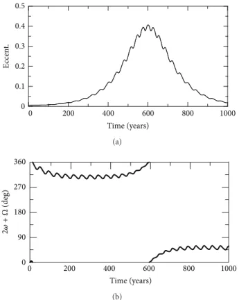
Figure 1: Time evolution of the eccentricity (a) and the critical angle (b). Initial conditions:� = 30, 647km,� = 0.005,� = 56.06∘, and other elements equal zero. In the simulations we consider only the sun and the oblateness of the earth as perturbations.

this work, as perturbations, we consider just the sun and the oblateness of the earth (the complete Cartesian equations involving the remaining perturbations will be given in the

next section).Figure 1shows the efects of the resonance on

the eccentricity and on the resonant angle. Note that an initial small eccentricity reaches a signiicant increase.

For the inclination� = 56.06∘, the dominant resonant

term in the double averaged solar disturbing function(̂�_⨀)is

cos(2� + Ω − Ω_⨀). Neglecting the remaining terms of̂�_⨀(a full development of the single and double averaged disturbing

function of the Sun is found in [13]), the Hamiltonian of the

problem is

� = ��2+

�2_� ⨀�2 2�3

⨀

× [�8 (1 − 3cos2(�) − 3cos2(�_⨀)

+9cos2(�)cos2(�_⨀))

− 34�sin(�)sin(�_⨀) (1 +cos(�))

×cos(�_⨀)cos(2� + Ω − Ω_⨀) ] , (4)

where�is the gravitational constant,�_⨀is the mass of the

sun, and�_⨀,�_⨀,Ω_⨀, are, respectively, the magnitude of the

position vector and the inclination and the ascending node of

the sun:� = 1 + (3/2)�2and� = (5/2)�2.

Taking� = √�2(�_�+ �)�,� = �√1 − �2,� = �cos(�),

� =mean anomaly,� = �, Ω = ℎ, the set of the

Delau-nay variables and performing a Mathieu canonical

transfor-mation [18], we have

̃�⨀= � 2_�

⨀�2 2�3

⨀

× [�8 (1 − 3(�1+ �2)2 4�2

1 − 3cos 2_(�

⨀)

+9(�1+ �2)2 4�2

1 cos

2_(� ⨀))

− 34�(1 −(�14�+ �22)2

1 )

1/2

sin(�_⨀)

× (1 + �1+ �2

2�1 )cos(�⨀)cos(�1) ] ,

̃��2= 14�

2_�

2�2�(3(�1+ �2) 2 4�2

1 − 1) (1 − �

2_{− 4�}2 1

�2 )

−3/2 ,

(5)

where�₁= 2� + Ω,�₁= �/2,�₂= Ω, and�₂= � − (�/2).

he orbit of the Sun is assumed to be Keplerian and we

also considered �_⨀ = 0, Ω_⨀ = 0. In (�_�, �_�) variables,

our Hamiltonian is a one-degree of freedom problem, whose dynamics is very similar to the Lidov-Kozai resonance. In

Figure 2 we consider an initial eccentricity �₀ = 0.005

and semimajor axis � = 30, 647km. his igure is very

instructive: note that in the bottom part there is a large region where the satellite remains some inite time with very small

eccentricity. It corresponds to the region where2� + Ω ≈ 0,

which is the region of interest for the minimum eccentricity

strategy study shown in [13]. On the other hand, we have

the counterpart of this situation at the top of the igure:

very high eccentricity, which occurs again for2� + Ω ≈ 0.

his is our region of interest, because we intent to use this increase of the eccentricity to discard the satellites. It is worth noting that if the semimajor axis is high, the efect of the moon cannot be neglected, so that the problem is no more a one degree of freedom problem. In this case the search of

the (�, Ω) pair such that the eccentricity increases must be

done by integrating the complete equations of motion. A full

characterization of this resonance is found in [13].

(4)

0 0.1 0.2 0.3 0.4 0.5 0.6 0.7

−180 −90 0 90 180

Eccen

tr

ici

ty

2� + Ω (deg)

Figure 2: Level curves of the Hamiltonian (̃�_⨀+ ̃��₂), showing the eccentricity variation versus resonant angle.

3. Initial Conditions for the Strategy of

Increasing the Eccentricity

In the previous section, we considered only the efects of the sun and the oblateness of the earth. Moreover, in the presence of the resonance, the main efects are now governed by the long term variations, since we considered the averaged problem. From a theoretical point of view, this averaged system is quite eicient to highlight the basic dynamics that afects the eccentricity of the GNSS satellites. However, for a more complete and realistic study, from now on, we need to include more perturbations.

In this section we want to ind some special initial conditions such that the eccentricity of the satellites reaches high values within an interval of 250 years. he strategy to search for these particular initial conditions is guided from the theoretical approach described in the previous section.

We integrate the exact equations of motion of the GNSS

satellites to be disposed (with inclination around 56∘), under

the efects of the sun, the moon, the geopotential with degree and order eight, and the radiation pressure coming from the Sun with eclipses. We use the RADAU integrator, a fast and

precise numerical code [19], written in FORTRAN language

and compiled using a Linux system.

he acceleration of the satellite using the exact system is

̈⃗� = −��

�3 ⃗� − ��⨀( ⃗� − ⃗�⨀ �� ⃗�− ⃗�⨀��3

− ⨀⃗� �� ⃗�⨀��3

)

− ��( ⃗� − ⃗�_{�� ⃗�− ⃗�}� ��3 − ⃗�

�

�� ⃗��3) + ⃗��+ ⃗��,

(6)

0 90 180 270 360

0 0.1 0.2 0.3 0.4 0.5 0.6

Eccen

tr

ici

ty

�0

(

deg

)

Ω0(deg)

Figure 3: he color scale shows the maximum eccentricity reached in 250 years of evolution of the orbit of the satellite. Initial conditions:� = 26, 559.74km,� = 0.005, and� = 56.06∘. he straight line satisies the relation2� + Ω = 0. Initial inclination of the moon is equal to 18.28∘. he dynamics consider the exact system.

where�is the gravitational constant,�_�,�_⨀,�_�are the

masses of the earth, the sun, and the moon, respectively.

⃗�

, _⨀⃗� , _�⃗� are, in order, the position vector of the satellite,

the sun, and the Moon. _�⃗� is the acceleration due to the

disturbing geopotential up to order and degree eight, which is enough to ensure suicient precision for this type of study

[20]. We use a recursive geopotential model [20–23], with the

coeicients of the EGM2008 (Earth Gravity Model) [24]. _��⃗�

is the acceleration due to the radiation pressure of the sun

with eclipses [25–27].

Figures 3 and 4 show the initial pair (�, Ω) and the

maximum eccentricity reached in 250 years. he other initial

elements are� = 26, 559.74km,� = 0.005, and� = 56.06∘.

We consider two values for the inclination of the moon,�_�=

18.28∘ _{and 28.58}∘_{, with respect to the mean equator of the}

earth, and we can see that the initial value of the inclination of the moon is important. he two straight lines represent the

exact condition2� + Ω = 0. Note that now we have added

the moon to our system, so that its efects can enhance the time variation of the eccentricity. he very smooth behavior

(eccentricity-resonant angle) seen inFigure 2certainly will

be lost as well as the position and the magnitude of the maximum and minimum values of the eccentricity. his is expected since now the satellite will be under the action of the disturbance of the moon whose efect is about two

times larger than the sun, as we will show inSection 5. We

also should point out that, in most of the cases shown in

Figures3and4, the eccentricity does not reach high values

(5)

0 90 180 270 360 0

90 180 270 360

0 0.1 0.2 0.3 0.4 0.5 0.6

Eccen

tr

ici

ty

�0

(

deg

)

Ω0(deg)

Figure 4: he same of the previous igure, but with��= 28.58∘.

Figure 5 shows the results for a complete set of initial conditions of a GPS satellite (US catalog 22108) for the epoch April 4, 2012. he initial conditions of the moon and the sun are adjusted for the same epoch, because the initial conditions of the perigee of the sun are signiicant (the quantitative impact of the inclination of the moon and the perigee of the

sun will be shown inSection 5). We note the growth of the

regions with high eccentricities. However, again, in all cases the time for the eccentricity growth is very large (200 years). A more realistic condition requires not only the increase of the eccentricity, but the decay of the periapsis radius to values below than 6,578 km (periapsis altitude of 200 km). his value

depends on the area to mass ratio of the satellite [28], and we

consider that ater the periapsis radius reach this value, the residual atmospheric drag will make the satellite reenter in the atmosphere. his value of periapsis is successfully used in studies of deorbiting of the GNSS satellites using

low-thrust propulsion and solar radiation pressure [1]. herefore,

in our simulations we are interested in obtaining sets of initial conditions that satisfy this precise concept, so that ater some preixed time, we can ensure that the satellites really end up reentering into the atmosphere of the earth.

In an attempt to reduce the time that the eccentricity demands to reach high values, we simulate orbits with a pair of initial semimajor axis and eccentricity so that the initial value of the apoapsis radius of the satellites is 10,000 km below the value of the apoapsis radius of the orbits presented in

Figure 5. he result is shown inFigure 6. Contrary to what is desired, note that the region with high values of eccentricity almost vanished. his can be explained by our averaged

model (4): the smaller is the semimajor axis (altitude), the

weaker is the efect of the2 ̇� + ̇Ω ≈ 0resonance; that is, for

satellites in lower orbits (small semi-major axis) the net efect

of this resonance is negligible, in spite of its existence.Figure 6

clearly shows this fact. In this sense, we take the opposite

scenario ofFigure 6, an initial pair of semimajor axis and

eccentricity so that the apoapsis radius is 10,000 km above the

value used inFigure 5.Figure 7shows these simulations and

0 0.2 0.4 0.6 0.8

Eccen

tr

ici

ty

0 90 180 270 360

�0

(

deg

)

Ω0(deg)

Figure 5: he same of Figures 3and 4. Initial conditions: � =

26, 561.1206km,� = 0.0220, and� = 56.2641∘(US catalog 22108).

��= 21.78∘_,_�

Sun= 105.43∘(Epoch 04/12/2012).

0 0.1 0.2 0.3 0.4 0.5

Eccen

tr

ici

ty

0 90 180 270 360

�0

(

deg

)

Ω0(deg)

Figure 6: he same ofFigure 5, but with apoapsis radius 10,000 km below the nominal value.

we can see that the regions with high eccentricity are larger than in the previous igures, as expected.

As explained before, an analysis of which initial

con-ditions inFigure 7 drive the periapsis altitude to less than

200 km is necessary. Figures8and9show the complementary

information for that.Figure 8 shows the regions where the

periapsis altitude decreases to values less than or equal to 200

km within 250 years. ComparingFigure 8withFigure 7, we

see that although the eccentricity can reach high values (0.8 for example), this is not enough to lower the periapsis altitude to penetrate into the atmosphere (in our case 200 km). More-over, to decide the best initial pair (perigee and longitude of ascending node) to discard a satellite, we also need to consider the amount of time which will be spent by the satellite to reach 200 km of periapsis altitude. he search of these conditions is easily done directly from the simulations.

In fact, fortunately, in the(�, Ω)plane, the region covered by

(6)

0 0.15 0.3 0.45 0.6 0.75 0.9

Eccen

tr

ici

ty

0 90 180 270 360

�0

(

deg

)

Ω0(deg)

Figure 7: he same ofFigure 5, but with apoapsis radius 10,000 km above the nominal value.

25 50 75 100 125 150 175 200

P

er

ia

psis al

ti

tu

de (km)

0 90 180 270 360

�0

(

deg

)

Ω0(deg)

Figure 8: Initial conditions(�, Ω)ofFigure 7in which periapsis altitude has reached at least 200 km (or less). In the white regions the periapsis altitude does not reach 200 km in 250 years of integration.

in blue color, we have an interesting view of the main initial

conditions. InFigure 10, the time evolution of one speciic

orbit is given. hus, increasing the semimajor axis of the satellite (via orbital transfer) so that the apoapsis radius raises, for example, 10,000 km above its nominal value, is a viable way to exploit the resonance to disposal the GNSS satellites. In the next section we make a comparison of the cost (in terms of the increment of velocity) between the disposal via resonance and the direct deorbiting.

In order to ensure that the method of increasing the apoapsis radius to enhance the efect of the 2 : 1 perigee-ascending node resonance works for all the satellites of the

GNSS with inclination around 56∘, we present Figure 11,

which show a satellite of the Galileo system (US catalog 28922) with a semimajor axis so that its apoapsis radius has

10,000 km above the nominal value. Analogously,Figure 12

shows a case for a satellite of the Beidou system (US catalog 31115) also with apoapsis radius 10,000 km above the nominal one.

0 25 50 75 100 125 150 175 200 225 250

T

ime (y

ea

rs

)

0 90 180 270 360

�0

(

deg

)

Ω0(deg)

Figure 9: Time required for the periapsis altitude to reach 200 km in integrations ofFigure 7as a function of the initial perigee and ascending node of the satellite. In the white regions the periapsis altitude does not reach 200 km during 250 years of integration.

Figures13and14show, respectively, the orbits ofFigure 11

which achieve 200 km of periapsis altitude and the time spent for these satellites to achieve 200 km of periapsis altitude.

Figures15and16present the same information forFigure 12.

4. The Direct Deorbiting Compared with the

Disposal via Resonance

he transfers chosen for the direct deorbiting and for the increase of the semimajor axis in the technique of disposal

via resonance are both of the Hohmann type [29], because, in

both cases, they are the simplest and fastest solution. Classically, the Hohmann transfer is coplanar and

con-sists in the application of two increments of velocity ΔV:

the irst one (ΔV_�) at the periapsis of the initial orbit (point

A, inFigure 17), that puts the satellite in the transfer orbit

(dashed), and the second one (ΔV_�) applied at the apoapsis

of the transfer orbit (point B) that puts the satellite in the inal orbit, which has the apoapsis coincident with that of the transfer orbit.

Some diferences appear between the original Hohmann transfer and the transfer that we use. Both orbits (initial and inal) are elliptical in our transfer, including the one for the direct deorbiting. he transfer occurs from point B to point

A, and the secondΔVdoes not exist, because we consider that

the satellite has already entered in the atmosphere.ΔV_�is in

the direction opposite to the motion of the satellite. For the disposal via resonance, the transfer occurs from the point A

to point B, butΔV_�is not required, because this transfer is

performed only to increase the apoapsis of the initial orbit. For the direct deorbiting, the apoapsis radius and the velocity at the point B of the orbit 3 are given by

��= �3(1 + �3) ,

V_�= √ 2�

�� − ��3,

(7)

0 10 20 30 40 50 60 Years

0 0.2 0.4 0.6 0.8

Eccen

t.

(a)

0 10 20 30 40 50 60

Years 6000

12000 18000 24000 30000

P

er

ia

p

sis radi

us (km)

(b)

Figure 10: Temporal evolution of the eccentricity (a) and the periapsis radius (b) of a satellite with initial conditions:� = 31, 557.9896km,

� = 0.17698,� = 56.2641,� = 22∘, andΩ = 236∘(marked by a black circle in Figures7,8, and9). he periapsis altitude reaches 200 km ater

50 years.

0 0.15 0.3 0.45 0.6 0.75 0.9

Eccen

tr

ici

ty

0 90 180 270 360

�0

(

deg

)

Ω0(deg)

Figure 11: Galileo satellite (US catalog 28922) with apoapsis radius 10,000 km above the nominal value. Initial conditions:� =

29, 716.46180km,� = 0.00079, and� = 56.2213∘.�� = 21.78∘,

�Sun= 105.43∘(Epoch 04/12/2012).

where�₃and�₃are the semimajor axis and the eccentricity of

the orbit 3 and�is the gravitational parameter of the Earth.

he periapsis radius(�_�) is the equatorial radius of the

earth and the apoapsis radius coincides with the apoapsis

of the orbit 3. hus, we can calculate the eccentricity�₂, the

angular momentum(�), and the velocity in the apoapsis(V₂)

of the orbit 2 [30]:

�2= �_��− �� + ��, � = √�� (1 + �2),

V₂= �

��.

(8)

he increment of velocity in B (and consequently the incre-ment to perform the direct deorbiting), is

ΔV_�=V_�−V₂. (9)

Table 1shows the results of the direct deorbiting transfers applied on some elements of the GNSS that have

incli-nations around 56∘ and that resides in MEO. he initial

conditions were collected in the Celestrak Catalog [31] and

correspond to the epoch April 18, 2012 and are shown in Table A1 in Supplementary Material available online at

http://dx.doi.org/10.1155/2014/382340. he initial conditions of the sun and the moon also correspond to the same epoch.

he US catalog number is the satellite identiication,�₀,�₀,

�0are the semimajor axis, inclination, and eccentricity of the

initial orbit,ΔV is the increment of velocity to execute the

transfer,� is the period of transfer, and� the eccentricity

of the inal orbit. Figure 18 presents the tridimensional

representation of the transfers for the satellites 20959 and

22014, where�,�, and�are the components of the radius

vector of these satellites.

he procedure to calculate theΔVto increase the apoapsis

in the disposal via resonance is quite similar to the previous calculation and is omitted here. he inal orbit in this case is more eccentric and this fact increases the solar perturbation. We impose a limit to the augment of the apoapsis radius, which is equal to the one used to deorbit a satellite at the same altitude. We also limit the apoapsis height in order to avoid

the crossing orbit with the GEO satellites.Table 2shows some

results of this transfer for the GNSS satellites, whereΔ�apois

the increment in the apoapsis radius,�_�and�_�are the inal

semimajor axis and eccentricity,�is the transfer time, andΔV

is the velocity increment that has to be applied to the satellite

in order to increase the apoapsis radius inΔ�apo. he time

of transfer does not include the time required to adjust the

(8)

Table 1: Results for the direct deorbiting transfers.

US catalog �0[km] �0[degree] �0 ΔV[km/s] �[h] �

20959 26560.7664 54.5454 0.011944 1.44298304067 2.9633 0.6164 22014 26560.1638 56.3669 0.020705 1.42793604813 2.9944 0.6191 22108 26561.1206 56.2641 0.022017 1.42568876224 2.9993 0.6195 22700 26559.8276 56.4089 0.017141 1.43388624044 2.9818 0.6180 28922 29716.4621 56.2213 0.000788 1.48398191129 3.3541 0.6468 32781 29544.1276 55.9161 0.002283 1.48036564168 3.3365 0.6456 37846 29600.2581 54.7324 0.000485 1.48368713514 3.3367 0.6456 37847 29600.2226 54.7332 0.000603 1.48346911163 3.3372 0.6456 31115 27910.1368 56.6975 0.000429 1.47338023307 3.1042 0.6281

Table 2: Results of the disposal via resonance transfer.

US catalog Δ�apo[km] ��[km] �� (h) ΔV[km/s]

22108 5000 29057.98957 0.10618 6.8466 0.1597965094

22108 10000 31557.98957 0.17699 7.7489 0.2896220183

22108 15000 34057.98957 0.23740 8.6877 0.3973314563

22108 20000 36557.98957 0.28955 9.6617 0.4882128746

22108 25000 39057.98957 0.33503 10.6695 0.5659710974

22108 30000 41557.98957 0.37503 11.7101 0.6332858627

28922 5000 32216.39876 0.07826 7.9927 0.1393530200

28922 10000 34716.39876 0.14463 8.9409 0.2547025152

28922 15000 37216.39876 0.20209 9.9238 0.3518810395

28922 20000 39716.39876 0.25232 10.9404 0.4349393122

28922 25000 42216.39876 0.29659 11.9895 0.5067891562

31115 5000 30409.75130 0.08258 7.3299 0.1522150787

31115 10000 32909.75130 0.15227 8.2521 0.2768316358

31115 15000 35409.75130 0.21212 9.2101 0.3808744430

31115 20000 37909.75130 0.26408 10.2024 0.4691299224

31115 25000 40409.75130 0.30961 11.2281 0.5449853332

any cost, by using the natural variation of these elements of the satellite, so, the time spent in this adjustment depends on how much the pair chosen is near the real values of these elements at the moment of the desired disposal.

Comparing the ΔV required by the direct deorbiting

with theΔVrequired by the disposal via resonance, we can

note that the most economical strategy is the disposal via

resonance, even for high values ofΔ�apo.

In order to demonstrate the entire process of the disposal via resonance, we take, as an example, the case of the satellite

22108 using 10,000 km of Δ�apo to make the disposal via

resonance. From Figures8and 9we can choose the initial

pair(�, Ω)that makes the satellite reach 200 km of periapsis altitude in the shortest time. his pair must be chosen as close as possible to the current value of the satellite, so, we save time

waiting for the satellite to reach the desirable value of(�, Ω),

due to the natural precession of�andΩ. As soon as these

values are reached, the maneuver to increase the apoapsis

radius is performed, raising the apoapsis radius by 10,000 km. he consequence of this process is to place a satellite in a more eccentric orbit (natural consequence of the maneuver), which reaches 200 km of periapsis altitude in 50 years (in this case). his time is comparable with the time that the upper stages of the rockets that send the satellites Beidou into orbit takes to

reenter in the atmosphere of the earth [32].

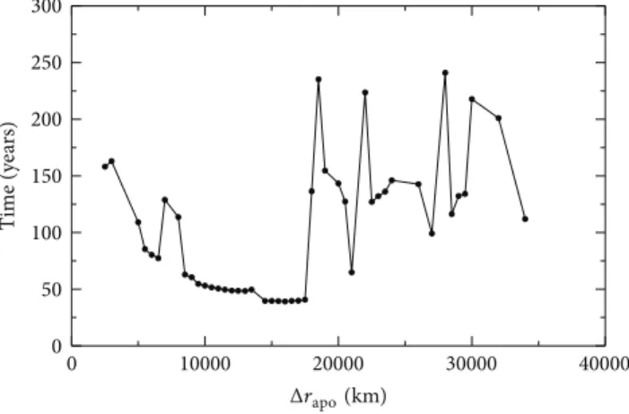
We can decrease the time of discard by taking other

values ofΔ�apoand keeping the same values of�andΩfrom

Figure 9. Figure 19 shows the time in which the periapsis radius reaches the value of 200 km of altitude during the

numerical integration for several values of Δ�apo. We can

verify that if we take a pair (�, Ω) in the unstable region

of Figure 8 (and consequently Figure 9) and increase the apoapsis radius, the time of disposal is reduced. However,

fromΔ�apo equal to 18,000, the time has an erratic

distri-bution, which leads to an optimum value ofΔ�apo around

(9)

0 0.15 0.3 0.45 0.6 0.75 0.9 Eccen tr ici ty

0 90 180 270 360

0 90 180 270 360 �0 ( deg )

Ω0(deg)

Figure 12: Beidou satellite (US catalog 31115) with apoapsis radius 10,000 km above the nominal value. Initial conditions: � =

27910, 13639km,� = 0.00043,� = 56.6975∘.�� = 21.78∘,�_Sun =

105.43∘_{(Epoch 04/12/2012).}

25 50 75 100 125 150 175 200 P er ia psis al ti tu de (km)

0 90 180 270 360

0 90 180 270 360 �0 ( deg )

Ω0(deg)

0 25 50 75 100 125 150 175 200 225 250 T ime (y ea rs )

0 90 180 270 360

0 90 180 270 360 �0 ( deg )

Ω0(deg)

25 50 75 100 125 150 175 200 P er ia psis al ti tu de (km)

0 90 180 270 360

0 90 180 270 360 �0 ( deg )

Ω0(deg)

0 25 50 75 100 125 150 175 200 225 250 T ime (y ea rs )

0 90 180 270 360

0 90 180 270 360 �0 ( deg )

Ω0(deg)

Δa → r_a → rb Δb A B 1 2 3

(10)

X (km₎

−20000 −10000

0

10000 20000

0

40000 20000 −20000

−30000 −10000 0 10000 20000 30000

Y(km )

Z(

km

)

−20000

Figure 18: Tridimensional representation of the Hohmann type maneuver executed for the satellites 20959 (black) and 22014 (red).

0 10000 20000 30000 40000

0 50 100 150 200 250 300

T

ime (y

ea

rs

)

Δrapo(km)

Figure 19: Time required for the periapsis radius to reach 200 km of altitude as a function of theΔ�_apo.

5. Quantitative Analysis of the Perturbation of

the Moon and the Sun

he integration of the equations of motion (6) can give

us interesting information about the inluence of the initial conditions of the moon and the sun on the evolution of the orbit of the satellite. We have seen that the inclination of the moon changes the dynamics of the resonance studied, and the value of the initial argument of the perigee of the sun also can afect the orbits of these satellites. By using the method of the integral of the forces over the time that was recently

proposed by Prado [15] that has many applications [16,20],

we can measure the magnitude of the acceleration due to the moon (as a function of its initial inclination) and to the sun (as a function of its initial argument of perigee) for several periods of time.

Ater the integration of the system, for an arbitrary period

of time�, by using the RADAU integrator, the magnitude

of the accelerations due to the perturbation of the moon and to the sun is stored. We integrate those magnitude of

the accelerations with the method of Simpson 1/3 [32] with

respect to the period of time�, obtaining the total velocity(�)

contribution of the disturbing body (Moon and Sun) during

the time interval�.

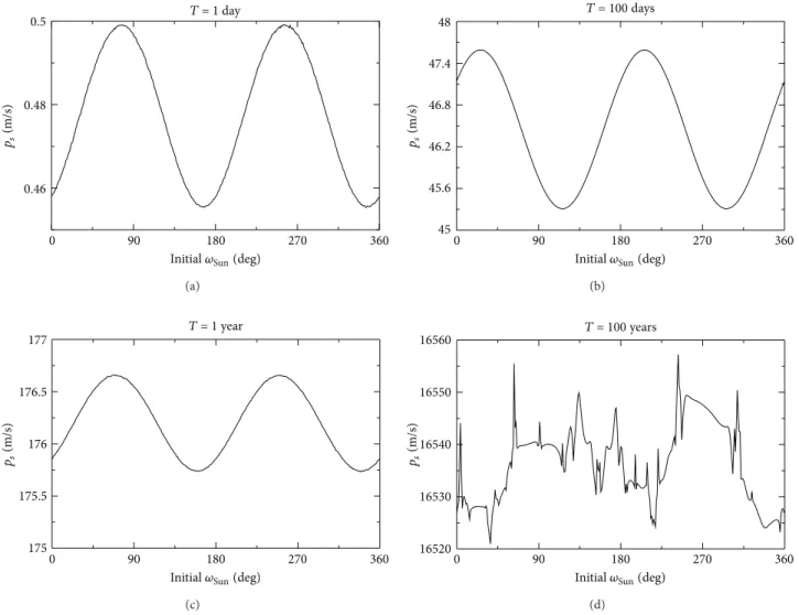
Figure 20shows the total velocity applied to a satellite of

the GNSS constellation due to the perturbation of the sun(�_�)

as a function of the initial perigee of the sun for 1 day (a), 100 days (b), 1 year (c), and 100 years (d). he predictability

of the efects ends in a period of around 70 years.Figure 21

shows the speciic total velocity due to the perturbation of

the moon(�_�)as a function of the initial inclination of the

(11)

0 90 180 270 360 0.46

0.48 0.5

Initial�Sun(deg)

T=1day

ps

(m/s)

(a)

45 45.6 46.2 46.8 47.4 48

0 90 180 270 360

T=100days

Initial�Sun(deg)

ps

(m/s)

(b)

175 175.5 176 176.5 177

0 90 180 270 360

T=1year

Initial�Sun(deg)

ps

(m/s)

(c)

16520 16530 16540 16550 16560

0 90 180 270 360

T=100years

Initial�Sun(deg)

ps

(m/s)

(d)

Figure 20: Variation of the integral of the acceleration due to the sun, with respect to the initial perigee of the sun. Initial condition of the satellite:� = 26, 561.1206km,� = 0.0220,� = 56.2641∘, and the other elements are equal to zero.

he predictability of the efects ends in a period of about 50

years. We can verify, comparing Figures20and21, that the

efect of the Moon is twice the efects of the Sun for the GNSS,

as expected. TroughFigure 21we also verify that the higher is

the inclination of the Moon, the greater is the perturbation on the GNSS satellite, which conirms what we mentioned in the previous sections. Also, the values of the total velocity due to the sun and the moon, can be useful in the creation of laws of control for the GNSS satellites, in order to attenuate the perturbations of the Sun and the Moon.

6. The Effect of the Resonance

2 ̇� + ̇Ω ≈ 0

over Beidou IGSO Satellites

he Beidou satellites are composed, as we mentioned before,

by satellites in MEO, with inclination near 56∘, GEO satellites,

and satellites in inclined geosynchronous orbits (IGSO), with

inclinations near 56∘. As we saw in the previous sections, in

this inclination, the resonance 2 : 1 perigee-ascending node can cause great increase in the eccentricity of the orbits of the satellites, even though these satellites are in near circular orbits. In the IGSO Beidou satellites, this increase in the eccentricity can amplify the risk of collision among

functional satellites. Figures22and23show the maximum

eccentricity achieved in 250 years (by integrating (6) with the

RADAU integrator) for the Beidou satellite 37210 (0.7716∘of

inclination) and 37384 (55.6720∘of inclination), respectively,

both with initial conditions corresponding to the epoch April 18, 2012. We can see that, for the satellite 37210, there is no signiicant increase in the inclination over the 250 years of integration, whereas the eccentricity of the satellite 37384

reached high values. he comparison between Figures22and

23shows us that the initial position of the pair(�, Ω)may be

(12)

18 20 22 24 26 28 30 Inclin. (deg)

0.96 0.961 0.962 0.963

0.964 T=1day

pL

(m/s)

(a)

104 104.5 105 105.5 106 106.5 107

18 20 22 24 26 28 30

Inclin. (deg)

T=100days

pL

(m/s)

(b)

380 384 388 392 396

18 20 22 24 26 28 30

Inclin. (deg)

T=1year

pL

(m/s)

(c)

36200 36250 36300 36350 36400

18 20 22 24 26 28 30

Inclin. (deg)

T=100years

pL

(m/s)

(d)

Figure 21: Variation of the integral of the acceleration due to the moon, as a function of the initial inclination of the moon. Initial condition of the satellite:� = 26, 561.1206km,� = 0.0220,� = 56.2641∘, and the other elements are equal to zero.

7. Conclusions

We found an alternative method to dispose the satellites of the GNSS which are in MEO and have inclinations around

56∘, by using the resonance 2 ̇� + ̇Ω ≈ 0 associated to

an orbital transfer to increase the apoapsis radius of the satellite to be disposable. We found sets of initial conditions such that the eccentricity of the satellite reaches high values, usually in less than 250 years. In comparison with the direct deorbiting, the alternative method has advantage in terms of fuel consumption, which is shown in terms of the increment of velocity that has to be applied to the satellite. he time required for the disposal is clearly shorter when compared to the time required to dispose the upper stages of the rockets used to place the satellites of the GNSS in orbit. Our technique provides the initial disposal conditions which lead to high values of eccentricity much faster than those presented in

previous work. he additional information of Figures8and9

guarantee the reentry in the atmosphere in the shortest possible time.

Although the focus of our work is the MEO satellites of the GNSS, and since the eccentricity grows faster when the satellite is closer to the sun, we wonder on the long term stability of the IGSO members of the Beidou constellation.

heir inclinations are close to 56∘and we show that the efects

of the resonance 2 ̇� + ̇Ω ≈ 0 are more intense for these

satellites. Based on the results, we suggest that the efects of the2 ̇� + ̇Ω ≈ 0resonance may be taken into account when the IGSO satellites are positioned in their nominal orbits in order to avoid the efects of the 2 : 1 perigee-ascending node resonance.

(13)

0 0.0002 0.0004 0.0006 0.0008 0.001 0.0012 0.0014 0.0016 0.0018 0.002 0.0022 0.0024

Eccen

tr

ici

ty

0 90 180 270 360

�0

(

deg

)

Ω0(deg)

Figure 22: he color scale shows the maximum eccentricity reached in 250 years of evolution of the orbit of the Beidou satellite (US catalog 37210). Initial conditions: � = 42, 165.13887km, � =

0.00060, and� = 0.7716∘.�� = 21.78∘,�_Sun = 105.43∘ (Epoch

04/18/2012). he dynamics consider the exact system (6).

0 0.2 0.4 0.6 0.8

Eccen

tr

ici

ty

0 90 180 270 360

�0

(

deg

)

Ω0(deg)

Figure 23: he same asFigure 22, but for the Beidou satellite (US catalog 37384). Initial conditions: � = 42, 165.81255km, � =

0.00212, and� = 55.6720∘.�� = 21.78∘,�Sun = 105.43∘ (Epoch

04/18/2012). he dynamics consider the exact system (6).

the future, for creating laws of control for the MEO satellites, in order to avoid seasonality in the perturbation of the sun and the moon.

Conflict of Interests

he authors declare that there is no conlict of interests regarding to the publication of this paper.

Acknowledgments

he authors wish to express their appreciation for the support provided by Grants nos. 473387/2012-3, 304700/2009-6, and 305834/2013-4, from the National Council for Scientiic and Technological Development (CNPq); Grants nos. 2012/21023-6 and 2014/02012/21023-62012/21023-688-7, from S˜ao Paulo Research Foundation (FAPESP), and the inancial support from the National

Council for the Improvement of Higher Education (CAPES). his research was supported by resources supplied by the Center for Scientiic Computing (NCC/GridUNESP) of the S˜ao Paulo State University (UNESP).

References

[1] E. M. Alessi, A. Rossi, G. B. Valsecchi et al., “Efectiveness of GNSS disposal strategies,”Acta Astronautica, vol. 99, pp. 292– 302, 2014.

[2] G. Beutler, Methods of Celestial Mechanics, Vol. II: Applica-tions to Planetary System, Geodynamics and Satellite Geodesy, Springer, Berlin, Germany, 2005.

[3] R. V. de Moraes, K. T. Fitzgibbon, and M. Konemba, “Inluence of the 2:1 resonance in the orbits of GPS satellites,”Advances in Space Research, vol. 16, no. 12, pp. 37–40, 1995.

[4] L. D. D. Ferreira and R. V. de Moraes, “GPS satellites orbits: resonance,”Mathematical Problems in Engineering, vol. 2009, Article ID 347835, 12 pages, 2009.

[5] R. R. Allan, “Resonance efects due to the longitude dependence of the gravitational ield of a rotating primary,”Planetary and Space Science, vol. 15, no. 1, pp. 53–76, 1967.

[6] A. Rossi, “Resonant dynamics of medium earth orbits: space debris issues,”Celestial Mechanics & Dynamical Astronomy, vol. 100, no. 4, pp. 267–286, 2008.

[7] NASA Safety Standard, “Guidelines and assessment procedures for limiting orbital debris,” Tech. Rep. NSS 1740.14, Oice of Safety and Mission Assurance, Washington, DC, USA, 1995. [8] C. C. Chao, “MEO disposal orbit stability and direct reentry

strategy,”Advances in the Astronautical Sciences, vol. 105, pp. 817–838, 2000.

[9] R. A. Gick and C. C. Chao, “GPS disposal orbit stability and sensitivity study,”Advances in Astronautical Sciences, vol. 108, pp. 2005–2018, 2001.

[10] C. C. Chao and R. A. Gick, “Long-term evolution of navigation satellite orbits: GPS/GLONASS/GALILEO,”Advances in Space Research, vol. 34, no. 5, pp. 1221–1226, 2004.

[11] A. B. Jenkin and R. A. Gick, “Dilution of disposal orbit collision for the medium earth orbit constellation,” in Proceedings of the 4th European Conference on Space Debris (ESA SP-587), D. Danesy, Ed., p. 309, ESA/ESOC, Darmstadt, Germany, April 2005.

[12] A. B. Jenkin and R. A. Gick, “Collision risk posed to the global positioning system by disposed upper stages,”Journal of Spacecrat and Rockets, vol. 43, no. 6, pp. 1412–1418, 2006. [13] D. M. Sanchez, T. Yokoyama, P. I. de Oliveira Brasil, and R.

R. Cordeiro, “Some initial conditions for disposed satellites of the systems GPS and Galileo constellations,”Mathematical Problems in Engineering, vol. 2009, Article ID 510759, 22 pages, 2009.

[14] C. Pardini and L. Anselmo, “Post-disposal orbital evolution of satellites and upper stages used by the GPS and GLONASS navigation constellations: the long-term impact on the Medium Earth Orbit environment,”Acta Astronautica, vol. 77, pp. 109– 117, 2012.

(14)

[16] A. F. B. A. Prado, “Mapping orbits around the asteroid 2001SN₂₆₃,”Advances in Space Research, vol. 53, no. 5, pp. 877– 889, 2014.

[17] T. Yokoyama, “Dynamics of some ictitious satellites of Venus and Mars,”Planetary and Space Science, vol. 47, no. 5, pp. 619– 627, 1999.

[18] C. Lanczos,he Variational Principles of Mechanics, University of Toronto Press, Toronto, Canada, 4th edition, 1970.

[19] E. Everhart, “An eicient integrator that uses Gauss-Radau spacing,” inDynamics of Comets: heir Origin and Evolution, vol. 115, pp. 185–202, Astrophysics and Space Science Library, 1985.

[20] D. M. Sanchez, A. F. B. A. Prado, and T. Yokoyama, “On the efects of each term of the geopotential perturbation along the time I: quasi-circular orbits,”Advances in Space Research, vol. 54, pp. 1008–1018, 2014.

[21] S. A. Holmes and W. E. Featherstone, “A uniied approach to the Clenshaw summation and the recursive computation of very high degree and order normalised associated Legendre functions,”Journal of Geodesy, vol. 76, no. 5, pp. 279–299, 2002. [22] A. Bethencourt, J. Wang, C. Rizos, and A. H. W. Kearsley, “Using personal computers in spherical harmonic synthesis of high degree Earth geopotential models,” inProceedings of the Dynamic Planet Meeting, Cairns, Australia, August 2005. [23] H. Kuga and V. Carrara, “Fortran- and C-codes for higher

degree and order geopotential and derivatives computation,” in16th Simp´osio Brasileiro de Sensoriamento Remoto, pp. 2201– 2210, Anais do SBSR, Foz do Iguac¸u, Brazil, 2013.

[24] N. K. Pavlis, S. A. Holmes, S. C. Kenyon, and J. K. Factor, “he development and evaluation of the Earth Gravitational Model 2008 (EGM2008),”Journal of Geophysical Research B: Solid Earth, vol. 117, no. 4, pp. 1978–2012, 2012.

[25] O. Montenbruck and E. Gill,Satellite Orbits: Models, Methods, and Applications, Springer, Berlin, Germany, 1st edition, 2001. [26] G. Beutler,Methods of Celestial Mechanics II: Application to

Planetary System, Geodynamics and Satellite Geodesy, Springer, Heidelberg, Germany, 1st edition, 2005.

[27] L. Anselmo and C. Pardini, “Long-term evolution of high earth orbits: efects of direct solar radiation pressure and comparison of trajectory propagators,” Tech. Rep. ISTI/CNR, 2007. [28] S. Campbell, C. C. Chao, A. Gick, and M. Sorge, “Orbital

stabil-ity and other considerations for U. S. Government Guidelines on Post-mission disposal of space structures,” inProceedings of the hird European Conference on Space Debris, 19–21 March 2001, Darmstadt, Germany, H. Sawaya-Lacoste, Ed., vol. 2 of

ESA SP-473, pp. 835–839, ESA Publications Division, Noord-wijk, he Netherlands, 2001.

[29] D. A. Vallado,Fundamentals of Astrodynamics and Applications, Space Technology Library, Hawthorn, Newzland, 3rd edition, 2007.

[30] H. D. Curtis,Orbital Mechanics for Engineering Students, Else-vier Butterworth-Heinemann, Boston, Mass, USA, 2005. [31] CELESTRAK,On Line Satellite Catalog (SATCAT), CSSI, 2012,

http://celestrak.com/.

(15)

Submit your manuscripts at

http://www.hindawi.com

Hindawi Publishing Corporation

http://www.hindawi.com Volume 2014

Mathematics

Journal of

Mathematical Problems in Engineering

Hindawi Publishing Corporation http://www.hindawi.com

Differential Equations

International Journal of

Volume 2014

http://www.hindawi.com Volume 2014 Mathematical PhysicsAdvances in

Complex Analysis

Journal of

Optimization

Journal of

Combinatorics

International Journal of

Journal of

Function Spaces

Abstract and Applied Analysis

International Journal of Mathematics and Mathematical Sciences

Hindawi Publishing Corporation http://www.hindawi.com Volume 2014

The Scientiic

World Journal

Discrete Dynamics in Nature and Society Hindawi Publishing Corporation

http://www.hindawi.com Volume 2014 Hindawi Publishing Corporation

Discrete Mathematics

Journal of

http://www.hindawi.com Volume 2014 Hindawi Publishing Corporation

Study of some strategies for disposal of the gnss satellites

Research Article