Theory of optical dispersive shock waves in photorefractive media
G. A. El,1,*A. Gammal,2,†E. G. Khamis,2,‡ R. A. Kraenkel,3,§and A. M. Kamchatnov4,储 1Department of Mathematical Sciences, Loughborough University, Loughborough LE11 3TU, United Kingdom
2
Instituto de Física, Universidade de São Paulo, 05315-970, C.P.66318 São Paulo, Brazil
3
Instituto de Fisica Teórica, Universidade Estadual Paulista, Rua Pamplona 145, 01405-900 São Paulo, Brazil
4
Institute of Spectroscopy, Russian Academy of Sciences, Troitsk, Moscow Region, 142190, Russia
共Received 11 June 2007; published 9 November 2007兲
The theory of optical dispersive shocks generated in the propagation of light beams through photorefractive media is developed. A full one-dimensional analytical theory based on the Whitham modulation approach is given for the simplest case of a sharp steplike initial discontinuity in a beam with one-dimensional striplike geometry. This approach is confirmed by numerical simulations, which are extended also to beams with cylindrical symmetry. The theory explains recent experiments where such dispersive shock waves have been observed.
DOI:10.1103/PhysRevA.76.053813 PACS number共s兲: 42.65.Tg, 42.65.Hw
I. INTRODUCTION
The study of optical solitons is a large area of modern research which is important both scientifically and for poten-tial applications共see, e.g.,关1,2兴兲. Different kinds of solitons have already been observed in various nonlinear optical me-dia, and their behavior has been explained in the frameworks of such mathematical models as the nonlinear Schrödinger
共NLS兲and generalized nonlinear Schrödinger共GNLS兲 equa-tions for different dimensions and geometries, so that one can consider the properties of single solitons as well enough understood.
However, there are situations when many solitons are generated so that they can comprise a dense soliton train. In such situations, it is impossible to neglect interactions be-tween solitons and one has to consider the evolution of the structure as a whole rather than to trace the evolution of each soliton separately. Usually, such soliton structures appear as a result of the wave breaking of a large enough initial pulse or large disturbance about a constant background. Hence, such structures can be considered as dispersive counterparts of shock waves well known in the physics of compressible viscous fluids共see, e.g.,关3兴兲. In a viscous fluid, the shock can be represented as a narrow region within which strong pation processes take place. In optics, on the contrary, dissi-pation effects can be neglected compared with dispersion ones and the shock discontinuity resolves into an expanding region filled with nonlinear oscillations. Such dispersive shock waves are known as tidal bores in rivers关4兴and have been also observed in some other physical systems including collisionless plasma 关5兴 and Bose-Einstein condensates 关6兴. Depending on the dispersive and nonlinear properties of the medium in which the wave propagates the dispersive shocks can be comprised of either bright or dark solitons. For
ex-ample, tidal bores consist of bright solitons governed by the Korteweg–de Vries equation for shallow-water waves whereas dispersive shocks in Bose-Einstein condensates with repulsive interatomic interaction are governed by the “defo-cusing” Gross-Pitaevskii equation and consist of a sequence of dark solitons.
It is important to note that dispersive shocks should not be confused with sequences of solitons generated in modula-tionally unstable media described, for instance, by a focusing nonlinear Schrödinger equation; see, e.g.,关7兴and references therein. Such media cannot exist in a uniform state, and any disturbance decays into bright solitons or even leads to a collapse in three-dimensional case. This situation in the op-tics of photorefractive crystals was discussed theoretically in
关8兴. In the present paper we consider the modulationally stable situation only.
Generation of multisoliton structures was observed in the propagation of light beams in nonlinear optical media关9–11兴. In these experiments, the initial nonuniformity of light beams necessary for formation of solitons was created by a large disturbance of either the intensity distribution or phase dis-tribution. In both cases an initial disturbance evolves into a sequence of solitons; the theory of a similar evolution for the Bose-Einstein condensate case described by a one-dimensional 共1D兲 Gross-Pitaevskii equation was developed in Ref.关12兴. Experiments on dispersive shock-wave produc-tion in optics have been recently reported in关13,14兴. Moti-vated by these experiments, we shall consider here the theory of dispersive shock waves in photorefractive media.
Since the number of interacting solitons in dispersive shocks is usually much greater than unity and these solitons are spatially ranked in amplitude, such a dispersive shock can be represented as a modulated periodic wave with pa-rameters changing a little in one transverse or longitudinal period of the envelope amplitude of the electromagnetic wave. A slow change of the parameters of the envelope am-plitude is governed to leading order by the Whitham modu-lation equations obtained by averaging conservation laws over the family of nonlinear periodic solutions or by the application of the averaged variational principle 共see, e.g.,
关3,15,16兴兲. For the one-dimensional NLS equation, the Whitham equations were derived in关17,18兴 共see also 关16兴兲
and the mathematical theory of dispersive shock waves for the defocusing case was developed in关19–25兴. It was applied to the propagation of signals in optical fibers in关26兴and in Bose-Einstein condensates in关6,27兴. It should be mentioned that for the case of the 1D NLS equation, the presence of an integrable structure has important consequences for the modulation共Whitham兲system; namely, the latter can be rep-resented in a diagonal共Riemann兲 form, which dramatically simplifies further analysis. The method of obtaining the Whitham equations in this form is based on the inverse scat-tering transform共IST兲applied to the NLS equation关17,18兴. However, in the case of the GNLS equation, the IST method cannot be used anymore and the diagonal structure of the Whitham system is not available. Nevertheless, it was shown in关28–30兴 that in this case, the main characteristics of the dispersive shock wave still can be found by using some gen-eral properties of the Whitham equations which remain present even in the nonintegrable case. Here we shall use this latter method for the derivation of parameters of one-dimensional dispersive shock waves generated in photore-fractive crystals and shall confirm our analytical results by numerical simulations, which also provide more detailed in-formation in the cases when the analytical approach is not yet developed共say, in 2D兲.
II. MAIN EQUATIONS
Photorefractive optical solitons were first observed in the experiment of 关31兴, and in the experiments of 关11,13兴 the formation of dispersive shock waves has been observed in the spatial evolution of light beams propagating through self-defocusing photorefractive crystals, so that beam nonunifor-mities give rise to breaking singularities and their resolution through dispersive shocks. As is known, the propagation of such stationary beams is described by the equation
i
z +
1 2k0
⌬⬜+k0
n0
␦n共兩兩2兲
= 0, 共1兲
whereis envelope field strength of electromagnetic waves with wave numberk0= 2n0/,zis the coordinate along the beam, x,y are transverse coordinates,r=共x,y兲, ⌬⬜=2/2x +2/2yis transverse Laplacian,n
0 is a linear refractive in-dex, and in the photorefractive medium we have
␦n= −1 2n0
3
r33Ep
+d
, 共2兲
whereEp is the applied electric field, r33 the electro-optical index,=兩兩2, and
dis a saturation parameter.
For mathematical convenience, we introduce nondimen-sional variables
z ˜=1
2kn0 2r
33Ep
冉
c
d
冊
z, ˜x=kn0
冑
1 2r33Ep冉
c
d
冊
x,
y
˜=kn0
冑
1 2r33Ep冉
c
d
冊
y, ˜=
冑
c, 共3兲wherecis a characteristic value of the optical intensity 共its concrete definition depends on the problem under
consider-ation; for instance, it can be the background intensity兲, so that Eq.共1兲takes the form
i
z +
1 2⌬⬜−
兩兩2
1 +␥兩兩2= 0, 共4兲 where␥=c/dand tildes are omitted. If the saturation effect is negligibly small共␥兩兩2Ⰶ
1兲, then this equation reduces to the usual NLS equation
i
z +
1
2⌬⬜−兩兩 2
= 0. 共5兲
It is convenient to represent these equations in a fluid-dynamics-type form by means of the substitution
共r,z兲=
冑
exp冉
i冕
r
u共r,z兲·dr
冊
, 共6兲so that they are transformed to
z+ⵜ⬜共u兲= 0,
uz+共uⵜ⬜兲u+ⵜ⬜f共兲−ⵜ⬜
冋
⌬⬜4 − 共ⵜ
⬜兲 2
82
册
= 0, 共7兲 wheref共兲=
1 +␥ for GNLS equation共4兲 共8兲
and
f共兲= for NLS equation共5兲. 共9兲
The light intensity in the hydrodynamic interpretation has the meaning of a density of a “fluid,” and Eqs.共8兲and
共9兲 can be viewed as “equations of state” for such a fluid. The functionu共r,z兲is a local value of the wave vector com-ponent transverse to the direction of the light beam; in hy-drodynamic representation, it has the meaning of the “flow velocity.” The variablezplays the role of time, so it is natu-ral to describe the deformations of the light beam in evolu-tionary terms. We note that the substitution共6兲rules out vor-ticity so that system 共7兲 actually represents a restriction of multidimensional NLS equation共5兲to potential “flows.” Ob-viously, if the initial distribution does not depend on one of the transverse coordinates共say,y兲, then transverse differen-tial vector operators reduce to the usual derivatives 共ⵜ
⬜ =/x,⌬
⬜=2/x2兲and Eqs.共7兲become an equivalent fluid dynamic representation of one-dimensional Eq.共5兲.
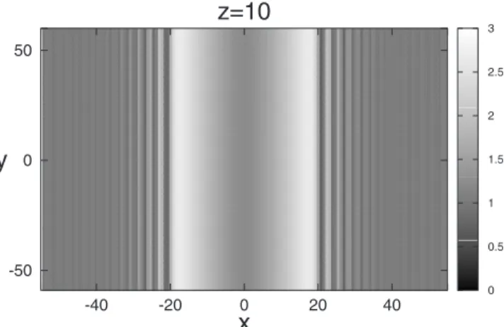
The evolution, according to Eq.共7兲of an initial distribu-tion, specified atz= 0, typically leads to wave breaking and the formation of dispersive shock waves. One can distinguish the following typical cases: 共i兲 generation of dispersive shocks in the evolution of a bright strip hump above a uni-form 共background兲 intensity distribution, 共ii兲 generation of sequences of solitons from a strip “hole” in the light inten-sity, and共iii兲generation of dispersive shocks in the evolution of a bright cylindrically symmetrical hump above a uniform intensity distribution.
are convenient for analytical considerations. As was shown in关6兴for the NLS equation case with␥= 0, this model agrees quite well with numerical simulations of 2D dynamics. Therefore we shall start here with these idealized models.
III. ANALYTICAL THEORY OF ONE-DIMENSIONAL DISPERSIVE SHOCKS GENERATED IN THE DECAY
OF A STEP LIKE INITIAL DISTRIBUTION
We shall start with an analytical treatment of shocks de-scribed by the 1D equation
iz+1
2xx−f共兩兩
2兲= 0 共10兲
or, in a fluid dynamics form, by the system
z+共u兲x= 0,
uz+uux+
df
dx+
冉
共x兲282 −
xx
4
冊
x= 0, 共11兲where the nonlinear refraction functionf共兲is given by Eq.
共8兲 or共9兲. Systems of the type共11兲are often referred to as dispersive hydrodynamics systems.
We consider the initial distributions of the intensity and transverse wave vectors in the form
共x,0兲=
再
0 forx⬍0,1 forx艌0,
冎
u共x,0兲= 0; 共12兲 that is, we assume that the initial velocityu共x, 0兲is equal to zero everywhere which means that the initial beam enters the photorefractive medium at z= 0 without any focusing. For the sake of definiteness we assume also that0⬎1.At the initial stage of evolution, linear waves are gener-ated which propagate according to the dispersion law ob-tained by means of linearization of Eqs.共11兲 about the uni-form state=0,u=u0共we keep here a nonzero value of u0 for future convenience兲; that is,=0+1exp关i共kx−z兲兴and
u=u0+u1exp关i共kx−z兲兴, where 1,u1Ⰶ1. Then a simple calculation yields
=0共0,u0,k兲=ku0±k
冑
0
共1 +␥0兲2 +k
2
4. 共13兲 Note that
⬙
共k兲⬎0, which implies the appearance ofdarksolitons in full nonlinear solutions. But before consideration of such solutions, we shall discuss a nonlinear stage of evo-lution in a dispersionless approximation when one can ne-glect the higher-order terms in the system共11兲. While in the case of general smooth initial data this stage of evolution is responsible for the formation of breaking singularities in the solution, its consideration also provides important insights into the nonlinear dissipationless dispersive dynamics of dis-continuous disturbances of the type 共12兲 even beyond the breaking point.
A. Dispersionless approximation
In dispersionless approximation, the system共11兲reduces to the standard equations of compressible fluid dynamics:
z+共u兲x= 0,
uz+uux+f
⬘
共兲x= 0. 共14兲 Because of the bidirectional nature of this system, generally, an initial step共12兲resolves into a combination of two waves propagating in opposite directions. One of these waves rep-resents a rarefaction wave with clear physical meaning, but the other one leads to a multivalued dependence of the in-tensity共x,z兲and transverse wave number共associated flow velocity兲 u共x,z兲 on the xcoordinate. Nevertheless, this for-mal global solution sheds some light on the structure of the actual physical solution and some its elements will be used later; therefore, we shall consider it here. To this end we cast the system 共14兲 into a diagonal form 共see, for instance,关3,16兴兲by the introduction of new variables, Riemann invari-ants
r±=u± 2
冑␥
arctan冑␥
, 共15兲so that it takes the form
r±
z +V± r±
x = 0, 共16兲
where the characteristic velocitiesV±are expressed in terms of the hydrodynamic variables andu by the relationship
V±=u±
冑
1 +␥. 共17兲
When␥→0 we haver±=u± 2
冑
,V±=u±冑
—i.e., the usual expressions for the dispersionless limit of the defocusing NLS equation共the shallow-water system—see, for instance,关19兴兲.
Since in the case of the steplike initial conditions the vari-ablesr±must depend on a self-similar variable=x/zalone, Eq.共16兲reduces to共V±−兲共dr±/d兲= 0 and we arrive at the so-called simple-wave solutions
u+
冑
1 +␥=x
z, u−
2
冑␥
arctan冑␥
=r− 0= const, 共18兲
or
u−
冑
1 +␥=x
z, u+
2
冑␥
arctan冑␥
=r+ 0= const. 共19兲
The constants here are chosen from the continuity conditions at the points where the simple waves enter the regions of constant intensities. Since the left-propagating rarefaction wave described by 共19兲 matches with the external flow
=0, u= 0 关see Fig. 1共a兲兴 we have r+ 0
=冑2␥arctan
冑
␥0 and, correspondingly,u= 2
冑␥
共arctan冑␥
0− arctan冑␥
兲. 共20兲冑
1 +␥+
2
冑␥
共arctan冑␥
− arctan冑␥
0兲= −x
z, 共21兲
which determines implicitly the intensity as a function of
x/z in the rarefaction wave. For x⬍x1− we have =0 = const, so x=x1− is the point of weak discontinuity which must propagate with sound velocity共see, for instance, 关32兴兲
which in our case is
cs共兲=
冑
1 +␥. 共22兲
Indeed, substituting =0 into Eq. 共21兲 we get x1 −
/z
= −cs共0兲. As a matter of fact, the speeds of the propagation of weak discontinuities in the photorefractive system agree with the group speeds determined by the long-wavelength limitk→0 in the linear dispersion relation共13兲.
Next, forx⬎x2− we have = 1, u= 0 关see Fig. 1共a兲兴 and this does not agree with the relationship 共20兲 in the con-structed left-propagating rarefaction wave solution. Hence, we have to introduce some intermediate distribution
共x/z兲=−
= const, u共x/z兲=u−= const, 共23兲
which matches with the rarefaction wave at some x=x1+. Now, to connect the intermediate distribution 共23兲 with
= 1,u= 0 downstream, we have to use the right-propagating
simple wave solution 共18兲 where the constant r+0
=冑2␥arctan
冑
␥. Hence we getu=
冑␥
2 共arctan冑␥
− arctan冑␥
兲 共24兲and
冑
1 +␥+
2
冑␥
共arctan冑␥
− arctan冑␥
兲=x
z. 共25兲
Equations 共20兲 and 共24兲 at =−
must give u=u−; hence, they yield the equation
arctan
冑␥
−= 12共arctan
冑␥
0+ arctan冑␥
兲, 共26兲 which determines the parameter−:
−=
冋
冑
1 +␥0− 1 +冑
0共冑
1 +␥− 1兲␥冑0−共
冑
1 +␥0− 1兲共冑
1 +␥− 1兲册
2. 共27兲
When−
is known, the parameteru−is found from Eq.共24兲,
u−= 2
冑␥
共arctan冑␥
−− arctan冑␥
兲. 共28兲The “internal” end pointsx1+andx2−are found by substituting the intermediate values−andu−into the similarity solutions
共18兲and共19兲,
x1+
z =u
− −
冑
−
1 +␥−,
x2−
z =u
− +
冑
−
1 +␥−. 共29兲 These points correspond to the weak discontinuities which propagate with sound velocitiescs共−兲in opposite directions in the reference frame associated with the uniform flowu−. The whole structure of intensity distribution is shown in Fig.
1共a兲. It has the regionx2−⬍x⬍x2+with the three-valued inten-sity, corresponding to the formal solution共18兲, which is ob-viously nonphysical and its appearance serves as an indica-tion that an oscillating dispersive shock wave is generated in the region of transition from =−,u=u− to += 1 ,u+= 0. The arising physical structure is shown schematically in Fig.
1共b兲. Importantly, the boundariesx2± of the oscillatory zone by no means coincide with those in the formal three-valued dispersionless solution. It is remarkable, however, that in spite of such a radical qualitative and quantitative change of the flow, the values of− andu−themselves turn out to be still determined by the previous equations共27兲and共28兲. This is a consequence of the dispersive shock jump condition which requires that the values of the Riemann invariantr− =u−共2 /
冑
␥兲arctan冑
␥ at both end points of the dispersive shock wave must be equal to each other:兩r−兩x2−=兩r−兩x2+, 共30兲 which gives at once Eq. 共28兲. Since the rarefaction wave, even in the presence of dispersion, is still described with good accuracy by the dispersionless approximation 共see
关33,34兴for the general linear asymptotic analysis of the dis-persive resolution of the weak discontinuities at the edges of
x x x x x
ρ = ρ
ρ = ρ
ρ = 1 ρ
0
-- + - +
1 1 2 2
(a)
ρ = ρ
0 ρ
ρ = ρ
ρ = 1
x- x x- x
-+ +
1 1 2 2
x
(b)
FIG. 1. Decay of the initial discontinuity of light intensity in a beam propagating through a photorefractive crystal.共a兲 Dispersion-less approximation with the nonphysical region of multivalued in-tensity.共b兲Schematic picture of the formation of dispersive shock due to the interplay of dispersive and nonlinear effects. The values ofx1−andx1+are the same for共a兲and共b兲while the values ofx2−and
the rarefaction wave兲, we deduce that Eq. 共27兲 obtained in the framework of the dispersionless fluid dynamics also re-mains valid. One should emphasize that, although all ob-tained relationships, strictly speaking, hold only asymptoti-cally for sufficiently large “times”z, as we shall see from the direct numerical solution, they hold with good accuracy for rather moderatez. The dispersive jump condition of the type
共30兲 was proposed for the first time in 关34兴 where it was based on intuitive physical reasoning and the results of nu-merical simulations of collisionless plasma flows. A consis-tent mathematical derivation of this condition along with some important restrictions to its applicability was given in the framework of the Whitham theory in关28,30兴.
As was mentioned, the end points of the oscillatory region of the dispersive shock in Fig.1共b兲do not coincide with the end points of the three-valued region in Fig. 1共a兲. Indeed, this oscillatory zone arises due to the interplay of dispersion and nonlinear effects and has a structure similar to that ob-served in the much-studied integrable defocusing NLS equa-tion case共see关19–27兴兲. Namely, near the leading edgex2+the wave transforms into a vanishing amplitude linear wave packet and at the trailing edge x2− it converts into a dark soliton. Hence, the end point of the oscillatory zonex2+must move with the group velocity of linear waves, cg=0/k, calculated for some nonzero value ofk=k+in contrast to the dispersionless approximation corresponding tok→0 共in ad-dition to a vanishing amplitude of oscillations a→0兲. The end pointx2− moves with the corresponding soliton velocity which also has nothing to do with the dispersionless limit
共note that in the soliton limitk→0 but the amplitude a=a−
remains finite兲. Thus, our task is to determine the main quan-titative characteristics of the oscillatory region of the disper-sive shock—the velocities of its end points as well as the amplitude a− of the trailing soliton at x=x
2 −
and the wave numberk+at the leading edge pointx=x
2 + .
One can observe that the oscillatory structure of the dis-persive shock wave is characterized by two different spatial scales: the intensity oscillates very fast inside the shock but the parameters of the fast oscillations change little in one wavelength in the x direction and in one period along the beam z axis. This suggests that the oscillatory dispersive shock can be represented as a slowly modulated nonlinear periodic wave and, hence, we can apply the Whitham modu-lation theory关3兴to its description. In the Whitham approach, the original equation containing higher-orderxderivatives is averaged over the family of nonlinear periodic traveling-wave solutions. As a result, one obtains a system of first-order nonlinear partial differential equations of hydrody-namic type 共i.e., linear with respect to first derivatives兲
governing the slow evolution of modulations. The modula-tion system does not contain any parameters of the length dimension, so it allows one to introduce the edgesx2±共z兲 of the dispersive shock wave in a mathematically consistent way, as characteristics where matching of the “internal”
共modulation兲and “external” 共dispersionless fluid dynamics兲
solutions occurs. Of course, strictly speaking, the averaged description is valid only when the ratio of the typical wave-length to the width of the oscillatory zone is small. For our case of the decay of an initial discontinuity this corresponds to a “long-time” asymptotic behavior,zⰇ1. However, as we
shall see from the comparison with a direct numerical solu-tion, the results of the modulation approach turn out to be valid even for rather moderate values ofz.
The modulation approach to the description of dispersive shock waves was realized for the first time by Gurevich and Pitaevskii 关33兴 in the framework of the Korteweg–de Vries
共KdV兲equation. To put this approach into practice for light beam deformations in a photorefractive medium, we first have to study periodic solutions of Eqs.共11兲.
B. Periodic waves and solitons in photorefractive crystals The traveling-wave solution of the system共11兲is obtained by the substitution =共兲, u=u共兲, where =x−cz is the phase and c= const is the phase velocity. As a result, we obtain by integrating the first equation of Eqs.共11兲,
u=c+A
, 共31兲
whereA is an arbitrary constant. Substituting Eq. 共31兲 into the second equation of Eqs.共11兲and performing one integra-tion with respect to we obtain an ordinary differential equation of second order,
1 8
冉
d
d
冊
2 =1
4
d2
d2− 2f共兲
−B2 −A
2
2 , 共32兲 whereBis another constant of integration. We shall seek its integral in the form
冉
dd
冊
2
=a1
冕
f共兲d+a22+a3+a4, 共33兲wherea1, a2, a3, and a4 are the constant coefficients to be found. Substituting Eq.共33兲 into Eq.共32兲we find, with the account of the specific dependencef共兲, the eventual form of the sought integral,
冉
dd
冊
2 = −8
␥2 ln共1 +␥兲+
冉
a2+ 8␥冊2
+a3+a4⬅Q共兲.
共34兲
Herea2,a3anda4, are arbitrary constants, two of which are connected withAandBby the relations
a2= 8B, a4= − 4A2, 共35兲 anda3is an additional constant so that Eq.共34兲is indeed the first integral of Eq.共32兲. We denote the roots of the equation
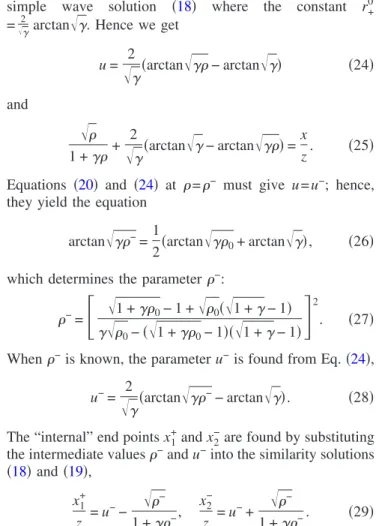
Q共兲= 0 ase1艋e2艋e3. Then the density oscillations in the traveling wave occur between e1 and e2. The amplitude of the wave is then given by a=e2−e1. The small-amplitude linear-wave configuration corresponds to e1→e2 while for solitons we havee2=e3. By imposing the periodicity condi-tion 共兲=共+ 2/k兲 we find the wave number k of the traveling wave in the form of the integral
k=
冉
冕
e1 e2
d
冑
Q共兲冊
−1
. 共36兲
solution in the form of a dark soliton. For this solution we must have the following boundary conditions satisfied at in-finity:
→b, u→ub, d/d→0,
d2/d2
→0 for兩兩→⬁, 共37兲
plus the condition d/d= 0 at=m艋b, where m is the value of the “density” in the minimum of the dark soliton andb is the “background” intensity. Applying these condi-tions to Eqs.共31兲 and共34兲 we obtain, after simple algebra, the expressions for the coefficients in Eq.共34兲for the soliton configuration,
a2= − 8b
1 +␥b− 4共ub−c兲
2,
a3= 8
␥2ln共1 +b兲− 8b
␥共1 +␥b兲
+4共ub−c兲 2共
m 2
+b 2兲
b
,
a4= − 4共ub−c兲2b 2
. 共38兲
The curvesQ共兲in a “soliton configuration” for several val-ues of␥are shown in Fig.2. The condition that in the soliton limit b be a double zero of the function Q共兲—that is,
dQ共兲/d= 0 at =b—yields the relationship between the soliton velocityc and the amplitudea=b−mfor given b andub:
共c−ub兲2= 2m
␥a
冋
1
␥aln
1 +␥b
1 +␥m−
1
1 +␥b
册
. 共39兲The dependence of the soliton velocity on the saturation pa-rameter␥ is shown in Fig.3.
For future analysis it is important to introduce one more parameter—the inverse half-width of the soliton—using the exponential decay of the intensityb− as 兩兩→⬁:
b−⬀exp共−兩兩兲, 兩兩→⬁. 共40兲 To find the relationship between and other parameters we take the series expansion of Q共兲 for small values of
⬘
=b− and find共d
⬘
/d兲2=共1 / 2兲共d2Q/d2兲b共⬘
兲2=2共⬘
兲2;hence,
=
冉
1 2冏
d2Q d2
冏
b冊
1/2
=
冋
8m+ 4␥b共b+m兲␥共b−m兲共1 +␥m兲2
− 8m
␥2共 b−m兲2
ln 1 +␥b 1 +␥m
册
1/2 .
共41兲
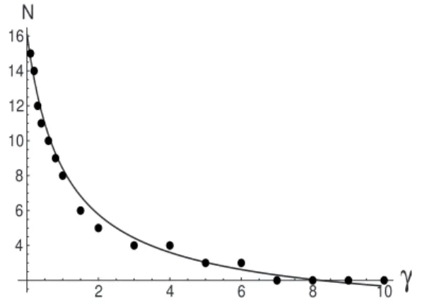
The dependence of on␥is shown in Fig. 4.
The profile of the intensity共兲 is determined by the in-tegral关see Eq.共34兲兴
=
冕
m
d
冑
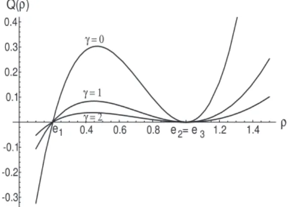
Q共兲, 共42兲where it is assumed that the intensity takes the minimal value =m at = 0 which determines the integration con-stant. The wave form of a dark soliton for different values of the parameter␥is shown in Fig. 5.
For␥Ⰶ1 we have the asymptotic expansions共for simplic-ity we takeub= 0兲
c=
冑
m冉
1 −␥
3共2b+m兲
冊
+O共␥ 2兲. 共43兲
0.4 0.6 0.8 1.2 1.4
-0.3 -0.2 -0.1 0.1 0.2 0.3 0.4
Q( )
ρ ρ
γ = 0
γ = 1
γ = 2
e1 e = e2 3
FIG. 2. Plots of the functionQ共兲 corresponding tob= 1 and
m= 0.2 and different values of ␥ and b= 1 and m= 0.2, so that
e1= 0.2,e2=e3= 1.
2 4 6 8 10
0.1 0.2 0.3 0.4 γ
γ c( )
FIG. 3. The plot of soliton velocity as a function of the satura-tion parameter␥. The other parameters areb= 1 andm= 0.2.
2 4 6 8 10
0.25 0.5 0.75 1 1.25 1.5 1.75
κ(γ)
γ
= 2
冑
b−m冋
1 −␥
3共3b+m兲
册
+O共␥ 2兲, 共44兲
and for␥Ⰷ1 other expansions
c=
冑
2兵m关ln共b/m兲− 1兴+m 2/b其
共b−m兲␥
+O共␥−2兲, 共45兲
=2
冑
b− 2mln共b/m兲−m 2/b
共b−m兲␥
+O共␥−3兲
. 共46兲
One can see that the leading terms in Eqs. 共43兲 and 共44兲
agree with the well-known dependences for dark solitons of the NLS equation关19兴.
The particular case of soliton solutions with m= 0 and
ub= 0共hencec= 0兲in photorefractive media has been found in关35兴.
C. Dispersive shock wave
The general periodic solution of the photorefractive equa-tion depends on the fast phase variableand is characterized by four parameterse1,e2,e3, andc, whereej, j= 1 , 2 , 3, are the zeros of the functionQ共兲, Eq.共34兲, which determine the profile of the intensity, and c is the phase velocity. In a modulated wave, these four parameters become slow vari-ables ofxandz. In the Whitham theory关3兴, it is postulated that this slow evolution 共modulation兲ej共x,z兲, c共x,z兲can be found from the conservation laws of the dispersive equation averaged over fast oscillations with respect to the phase vari-able. An additional modulation equation naturally arises as the wave number conservation lawkz+x= 0 and essentially represents a condition of the existence of a slowly modulated periodic wave共see, for instance,关3兴兲. Several averaging pro-cedures have been proposed, yielding equivalent results for various physical systems共see 关15兴兲, so the Whitham modu-lation theory can be now considered as quite well estab-lished. As a result, using the original procedure of averaging conservation laws, the Whitham system for the GNLS equa-tion can be obtained in the following general form:
关Pi共e1,e2,e3,c兲兴z+关Qi共e1,e2,e3,c兲兴x= 0, i= 1,2,3,
共47兲
关k共e1,e2,e3,c兲兴z+关共e1,e2,e3,c兲兴x= 0, =kc. 共48兲 HereP1=,P2=u, andP3=u are the conserved “densities” of the GNLS equation 共7兲 and Qi, i= 1 , 2 , 3, are the corre-sponding “fluxes.” The averaging is performed over the pe-riodic family共31兲and共34兲according to
f¯共e1,e2,e3,c兲=
k
冕
e1 e2 f共;e1,e2,e3,c兲
冑
Q共兲 d. 共49兲Now the system 共47兲 and 共48兲 is, in principle, completely defined.
The modulation system共47兲and共48兲being the system of hydrodynamic type can be hyperbolic 共real characteristic velocities—modulationally stable case兲 or elliptic共complex characteristic velocities—modulationally unstable case兲. It is known very well共see关16–18兴兲that for the defocusing NLS equation, which is an integrable particular case of the the GNLS equation共4兲, the modulation system is strictly hyper-bolic. Our numerical simulations show that traveling waves in the GNLS equation are modulationally stable and this sug-gests that the corresponding Whitham system is hyperbolic as well. So, in what follows, we shall assume hyperbolicity of the Whitham system, which will allow us to use some arguments of classical characteristics theory关3,32,36兴.
Now, to describe analytically the dispersive shock wave as a whole, we have to solve four modulation equations共47兲
and共48兲for the slowly varying parameterse1,e2,e3, andcof the periodic solution. These equations must be equipped with special matching conditions to guarantee continuity of the mean flow at the free boundariesx±共z兲defining the edges of the dispersive shock wave. In view of the numerically estab-lished qualitative spatial structure of the photorefractive dis-persive shock wave关see Fig.1共b兲兴we require that
atx=x+共z兲: a= 0, ¯=+, ¯u=u+, 共50兲
atx=x−共z兲: k= 0, ¯=−, ¯u=u−, 共51兲 wherex+⬅x
2 +共
from now on we shall omit the subscript 2 in
x2−andx2+兲. The dependences of¯,¯u,k, anda one1,e2,e3, andcare defined by Eq.共49兲and the formulas of Sec. III B, and the pairs 共−,u−兲 and共+,u+兲 represent the solution of the dispersionless approximation 共14兲evaluated at the trail-ing and leadtrail-ing edges of the dispersive shock wave, respec-tively. The edges x±共z兲 of the dispersive shock wave repre-sent free boundaries defined by the kinematic boundary conditions with clear physical meaning explained in Sec. III A:
dx+ dz =cg共
+
,u+,k+兲, dx −
dz =csol共
−
,u−,a−兲, 共52兲
wherecg共+,u+,k兲=
0/kis the group velocity of the lin-ear wave packet with the dominant wave numberk propagat-ing against the hydrodynamic background+
andu+关see Eq.
共13兲 for the linear dispersion relation =0共0,u0,k兲兴 and
csol共−,u−,a兲 is the velocity of the dark soliton with ampli-tudeapropagating against the background−andu−关see Eq.
共39兲for the dependence of the soliton velocity on its ampli-tude兴. Of course, the values of the wave number k+ at the
-10 -5 5 10
0.2 0.4 0.6 0.8
ρ
θ
γ = 0 γ = 1
γ = 2
leading edge and the amplitudea−of the trailing dark soliton are both to be determined, so the determination of the edges
x±共z兲represents a part of this nonlinear boundary value prob-lem.
Following the pioneering work of Gurevich and Pitaevskii
关33兴on the dispersive shock-wave description in the frame-work of the KdV equation, the effective methods for treat-ment of such problems have been developed for the whole class of evolution equations which share with the KdV equa-tion the unique property of complete integrability共see, e.g.,
关16兴兲. On the level of the Whitham equations, one of the manifestations of integrability is the presence of the full sys-tem of Riemann invariants, an event generally highly un-likely for the systems of hydrodynamic type with number of equations exceeding 2. In particular, the NLS equation 共5兲
belongs to this class, and the corresponding theory of disper-sive shock formation was developed in关19–25兴and success-fully applied to the description of shocks in nonlinear optics
关26兴 and Bose-Einstein condensates 关6,27兴. However, the photorefractive equation共4兲is not completely integrable and therefore the methods based on the presence of rich underly-ing algebraic structure of such equations cannot be applied here. Nevertheless, as was shown in关28–30兴, the main quan-titative characteristics of the dispersive shock wave can be derived using the general properties of the Whitham equa-tions共47兲and共48兲reflecting their origin as certain averages, and here we shall apply this method to the description of dispersive shock waves in photorefractive media. To be spe-cific, we shall be interested in the locations of the edges of the dispersive shock wave and in the amplitude of the largest
共deepest兲soliton at the trailing edge, the parameters that are usually observed in experiment.
The method of Refs.关28–30兴, which will be used below, is formulated most conveniently in terms of the physical modulation parameters¯,¯u,k, andaappearing in the match-ing conditions共51兲and共50兲. The key of the method lies in the fact that the modulation system共47兲and 共48兲, dramati-cally simplifies in the cases 共a= 0,k⫽0兲 and 共k= 0, a⫽0兲
corresponding to the limiting wave regimes realized at the boundaries of the dispersive shock wave.
1. Leading edge
At the leading edgex=x+共z兲the amplitude of oscillations vanishes, a= 0. Since the Whitham averaging procedure re-mains valid for the case a= 0 共averaging over the periodic family with vanishing amplitude兲, then we conclude that the Whitham system must admit anexactreduction ata= 0 and, therefore, the system of four Whitham equations must reduce here to only three equations. Now, if the amplitude of lations vanishes, then the average of a function of the oscil-lating variable equals to the same function of the averaged variable: F共,u兲=F共¯,¯u兲. Thus, when a= 0 the Whitham system must agree with the dispersionless approximation
共14兲 describing large-scale nonoscillating flows; i.e., the modulation equations for¯,¯u anda reduce to
a= 0, ¯z+共¯u¯兲x= 0, ¯uz+¯uu¯x+f
⬘
共¯兲¯x= 0. 共53兲 We note that this reduction of the Whitham equations is also consistent with the matching condition 共50兲 at the leadingedge of the dispersive shock wave where a= 0 and which requires that the solution of the Whitham equations must match the solution of the equations of the dispersionless ap-proximation. Of course, Eqs. 共53兲 can be derived directly from the modulation equations共47兲by passing in them to the limit a=e2−e1→0 共see, for instance, 关39兴 for the corre-sponding calculation in the context of fully nonlinear shallow-water waves兲; however, the validity of Eqs.共53兲 ap-pears to be obvious from the presented qualitative reasoning. To complete the zero-amplitude reduction of the modula-tion system we need to pass to the same limit asa→0 in the “number of waves” conservation law共48兲 in which we as-sume the aforementioned change of variables
共e1,e2,e3,c兲哫共¯,¯u,k,a兲,
kz+关共¯,u¯,k,a兲兴x= 0, =kc. 共54兲
As a result, we get
kz+关0共¯,¯u,k兲兴x= 0, 共55兲
where
0共¯,¯u,k兲=k
冉
¯u+冑
¯
共1 +␥¯兲2+
k2
4
冊
共56兲is the dispersion relation 共13兲 of linear waves propagating about a slowly varying background with locally constant val-ues of ¯ and ¯u 共here we restrict ourselves to right-propagating waves兲. Equations 共53兲 and 共55兲 comprise a closed system which represents an exact zero-amplitude re-duction of the full Whitham system 共47兲 and 共48兲 共see
关28,30兴for a detailed justification of this reduction for a class of weakly dispersive nonlinear systems兲and, as we shall see, its analysis with an account of boundary conditions共50兲and
共51兲yields the necessary information about the leading edge
x=x+共z兲of the dispersive shock wave.
Now we observe that the “ideal” hydrodynamic equations
共53兲 are decoupled from Eq.共55兲 and, thus, can be solved independently for¯共x,z兲,¯u共x,z兲. However, since the values of¯ and¯u at a= 0 are subject to boundary conditions共50兲, one should take into account the restriction on the admissible values of¯and¯uat the boundaries of dispersive shock wave imposed by the simple-wave transition condition共30兲. Since this restriction is consistent with Eqs.共53兲, it can be incor-porated directly into the reduced modulation system by put-ting
u
¯=
冑␥
2 共arctan冑
␥¯− arctan冑␥
兲. 共57兲Substitution of Eq.共57兲into the system共53兲and共55兲further reduces it to only two differential equations
¯z+V+共¯兲¯x= 0, kz+关⍀共¯,k兲兴x= 0, 共58兲
where
V+共¯兲= 2
冑␥
共arctan冑
␥¯− arctan冑␥
兲+冑
¯⍀共¯,k兲=0„¯,u¯共¯兲,k…=k
冋
2冑␥
共arctan冑
␥¯− arctan冑␥
兲+
冑
¯共1 +␥¯兲2+
k2
4
册
. 共60兲 The system共58兲has two families of characteristics:dx
dz=V+共¯兲 共61兲
and
dx
dz=
⍀共¯,k兲
k . 共62兲
The family 共61兲 is completely determined by the simple-wave evolution of the function¯共x,z兲 according to the dis-persionless approximation of the GNLS equation. This fam-ily transfers “external” hydrodynamic data into the dispersive shock-wave region and does not depend on the oscillatory structure. Contrastingly, the behavior of the char-acteristics belonging to the family 共62兲 depends on both¯
andk. Comparison of the definition共52兲of the leading edge
x+共z兲 with Eq.共62兲with the account of Eq. 共60兲shows that the leading edge of the dispersive shock wave represents a characteristic belonging to the family共62兲. Now, since the system共58兲consists of two equations, then according to gen-eral properties of characteristics of nonlinear hyperbolic sys-tems of partial differential equations 共see, for instance,
关3,32,36兴兲, one cannot specify two values k and¯ indepen-dently of one characteristic, so the admissible combinations of¯ andkat the leading edge of the dispersive shock wave are determined by a characteristic integral of the reduced modulation system共58兲.
To this end, we substitutek=k共¯兲into Eqs.共58兲to obtain at once
a= 0: dk
d¯ =
⍀/¯
V+−⍀/k on dx dz=
⍀
k. 共63兲
The above ordinary differential equation forkmust be solved with the initial conditionk共−兲
= 0. Indeed, since Eq.共63兲was derived for the casea= 0, it must remain valid in the case of the dispersive shock wave of zero intensity, so the depen-dencek共¯兲should correctly reproduce the zero-wave-number condition at the trailing edge where¯=−关see Eq. 共51兲兴.
By introducing the variable
␣=
冑
1 +k 2共1 +␥¯兲2
4¯ , 共64兲
instead of k, in 共63兲, and using Eq. 共60兲, we arrive at the ordinary differential equation
d␣
d¯ = −
共1 +␣兲关1 + 3␥¯+ 2␣共1 −␥¯兲兴
2¯共1 +␥¯兲共1 + 2␣兲 , 共65兲
with the initial condition
␣共−兲= 1, 共66兲
where− is determined in terms of the initial discontinuity
共12兲by Eq.共27兲. Once the solution␣共¯兲is found, the wave numberk+at the leading edge, where¯=+
= 1, is determined from Eq.共64兲as
k+=k共1兲=2
冑␣
2共1兲− 1
1 +␥ . 共67兲
The velocity of propagation of the leading edge is defined by the kinematic condition共52兲, which, with an account of Eq.
共62兲, assumes the form
s+=dx +
dz =
⍀
k共1,k
+兲
= 1
1 +␥
冉
2␣共1兲−1
␣共1兲
冊
. 共68兲For the NLS equation case—i.e., when␥= 0—the expres-sion fors+in terms of the density jump across the dispersive shock wave can be obtained explicitly: the equation
d␣
d¯ = −
1 +␣
2¯ , ␣共
−兲
= 1, 共69兲
is readily integrated to give
␣共¯兲= 2
冑
−
¯ − 1 共70兲
and thus
s+=8 −
− 8
冑
−+ 12
冑
−− 1 for␥= 0, 共71兲 in agreement with known results关19兴.For small values of the saturation parameter␥Ⰶ1 one can find the correction to this formula with the use of Eqs.共65兲
and 共68兲. Indeed, if we introduce ␣=␣0+␣1, where ␣0 is given by Eq.共70兲 and␣1 has the order of magnitude of ␥, then the series expansion of Eq. 共65兲yields the differential equation for the correction␣1:
d␣1
d¯ = − ␣1
2¯+
8
冑
− /¯− 6 4冑
−/¯− 1
冑
−
¯ ␥, 共72兲
which can be easily solved with account of the initial condi-tion␣1共−兲= 0 to give
␣1共1兲= 2␥冑−
再
1 −−+ 64冋
ln4
冑
−− 1 3冑
− +1 −
冑
− 4冑
−+1 − −
32−
册
冎
. 共73兲Then substitution of this expression into Eq. 共68兲 gives an explicit approximate formula fors+:
s+⬇8
−
− 8
冑
−− 12
冑
−− 1 共1 −␥兲+冋
2 − 1共2
冑
−− 1兲2册
␣1共1兲,共74兲
2. Trailing edge
In the vicinity of the trailing edge x=x−共z兲 the photore-fractive dispersive shock wave represents a sequence of weakly interacting dark solitons propagating on the slowly varying background¯ and¯u. Since one hask→0 asx→x−, we shall be interested in passing to a soliton limit in the modulation system共47兲and共48兲. Instead of performing this limiting passage by a direct calculation共which can be quite involved technically兲, we shall invoke a reasoning similar to that used in the study of the zero-amplitude regime to inves-tigate a reduced modulation system ask→0.
In the limit ask→0, the distance between solitons共i.e., a wavelength 2/k兲 tends to infinity, so the contribution of solitons to the averaged flow¯and¯uvanishes, and similarly to the case of the vanishing amplitude, we have F共,u兲
=F共¯,¯u兲. Hence, we arrive again at the ideal hydrodynamics system共53兲for¯ and¯u. Next, using the arguments identical to those used earlier for the casea= 0, but applied now to the casek= 0, we conclude that, for the matching condition共51兲
at the trailing edge to be consistent with the simple-wave transition condition共30兲 we should incorporate the relation
共57兲into the reduced as k→0 modulation system to obtain the same equation for¯ 关see Eq.共58兲兴, which we reproduce one more time:
¯z+V+共¯兲¯x= 0. 共75兲 Now we need to pass to the limit ask→0 in the wave conservation law. This limiting transition, unlike that as a
→0, is a singular one, so it requires a more careful consid-eration. First we note that the wave conservation law is iden-tically satisfied for k= 0, so we need to take into account higher-order terms in the expansion of Eq.共54兲for smallk. Following关28,30兴we introduce a “conjugate wave number”
k ˜=
冉
冕
e2 e3
d
冑
−Q共兲冊
−1
共76兲
instead of the amplitudeaand the ratio⌳=k/˜kinstead of the original wave number k, so that the parameters 共¯,¯u,⌳,˜k兲
provide a new set of modulation parameters which is conve-nient for consideration of the vicinity of the soliton edge of a dispersive shock. The variable˜kcan be considered as a wave number of oscillations of the variable in the interval e2 艋艋e3 governed by the “conjugate” traveling-wave equa-tion
冉
dd˜
冊
2
= −Q共兲, 共77兲
where Q共兲 is defined in Eq. 共34兲 and ˜ is a new phase variable. In the soliton limite2→e3 we can expandQ共兲in the vicinity of its minimum point¯=e2=e3 so that Eq.共77兲 takes the form of the “energy conservation law” of the har-monic oscillator,
1 2
冉
d
d˜
冊
2 +1
4
冏
d2Q
d2
冏
¯
共−¯兲2
=Q共¯兲= 0.
Then comparison with Eq.共41兲shows that in this limit
k ˜=
冑
12
冏
d2Q
d2
冏
¯=, 共78兲
which explains the physical meaning of the variable˜kin the limit we are interested in. This analogy can be amplified by noticing that Eq.共77兲 can be viewed as the traveling-wave equation corresponding to the “conjugate” GNLS equation obtained from Eq.共4兲by replacing the variablesxandzbyix
andiz, respectively, so that in Eq. 共34兲is replaced by i˜, which leads to the change of sign in Eq.共34兲 transforming this equation into Eq. 共77兲. Now, the same transformation maps a harmonic wave exp关i共kx−z兲兴to the tails of the soli-ton solution exp关±共x−csolz兲兴; that is, in the soliton limit the conjugate frequency˜0 can be obtained from the harmonic dispersion relation by a substitution
i˜0=0共i兲. 共79兲 Actually, this fact is well known and can be used for the calculation of the dependence of the soliton velocity csol
=˜0/ on its inverse half-width from the dispersion rela-tion for linear waves共see, e.g.,关37兴兲. Thus, for photorefrac-tive dark solitons propagating along the slowly varying back-ground¯ andu¯ we have the conjugate dispersion relation
˜0共¯,¯u,兲=
冉
¯u+冑
¯
共1 +␥¯兲2−
2
4
冊
, 共80兲which, after substitution of the simple-wave relation 共57兲, assumes the form关cf. Eq.共60兲兴
⍀˜共¯,兲=˜0„¯,¯u共¯兲,…
=
冋
2冑␥
共arctan冑
␥¯− arctan冑␥
兲+
冑
¯共1 +␥¯兲2−
2
4
册
. 共81兲Now we are ready to study the asymptotic expansion as k
→0 of the wave conservation law 共54兲. First we substitute
k=⌳˜kinto Eq.共54兲to obtain
k ˜⌳
⌳
z +
⍀˜
⌳
x = 0, 共83兲
which is to say
⌳=⌳0 on
dx dz=
⍀˜共¯,兲
, 共84兲
where ⌳0Ⰶ1 is a constant. In particular, when ⌳0= 0 the characteristic共84兲specifies the trailing edge 关see Eq.共52兲兴. Now, considering Eq. 共82兲 along the characteristic family
dx/dz=⍀˜/ and using˜k=,˜=⍀˜ to leading order, we ob-tain
z+⍀˜x= 0 on
dx
dz=
⍀˜共¯,兲
. 共85兲
We note that the equationz+⍀˜x= 0 arises as a “soliton wave number” conservation law in the traditional perturbation theory for a single soliton共see, for instance, 关38兴兲but to be consistent with the full modulation theory it should be con-sidered along the soliton pathdx/dz=csol=⍀˜/.
Since¯ and cannot be specified independently on one characteristic, there should exist a local relationship 共¯兲
consistent with the system 共75兲 and 共85兲. Substituting
=共¯兲 into共85兲and using共75兲we obtain
d
d¯=
⍀˜/¯ V+−⍀˜/
. 共86兲
The initial condition for the ordinary differential equation
共86兲follows from the requirement that the obtained depen-dence 共兲 should be applicable to the case of the zero-intensity dispersive shock wave, which corresponds to initial values−=+= 1. In this case, the width of solitons gets in-finitely large—that is,→0 in the limit→+; this follows also from Eq. 共41兲 in the limit m→b. Hence we require
共1兲= 0.
According to the kinematic condition共52兲the velocity of the soliton edge is equal to the soliton velocity, so we have
s−= dx −
dz =
⍀˜共− ,−兲
− , 共87兲
where−=共−兲.
By introducing a new variable
␣
˜=
冑
1 − 2共1 +␥¯兲2
4¯ 共88兲
instead of , Eq. 共86兲 reduces to the ordinary differential equation
d␣˜
d¯ = −
共1 +␣˜兲关1 + 3␥¯+ 2␣˜共1 −␥¯兲兴
2¯共1 +␥¯兲共1 + 2␣˜兲 , 共89兲
with the initial condition
␣
˜共1兲= 1. 共90兲
When the function␣˜共兲is found, the velocity of the trailing soliton is determined by Eqs.共81兲,共87兲, and 共88兲as
s−=
冑␥
2 共arctan冑␥
−− arctan冑␥
兲+冑
−1 +␥−␣˜共 −兲
. 共91兲
Then the amplitude a=−−
m of the trailing soliton as a function of the intensity jump−across the dispersive shock can be found from Eq.共39兲withc=s−,ub=u−, and b=−:
−␣˜2共−兲
共1 +␥−兲2= 2共−
−a兲
␥a
冋
1
␥aln
1 +␥− 1 +␥共−
−a兲−
1 1 +␥−
册
.共92兲
Again, in the case ␥= 0 corresponding to the NLS equa-tion, all formulas can be written down explicitly: Equation
共89兲reduces to
d␣˜
d¯ = −
1 +␣˜
2¯ , 共93兲
and its solution satisfying the boundary condition共90兲is
␣
˜共¯兲=
冑
2
¯ − 1. 共94兲
Then Eqs.共91兲and共92兲give
s−=
冑
− 共95兲and
a= 4共
冑
−− 1兲, 共96兲
respectively, in agreement with known results关19兴. Again for small␥ we can find the correction to Eq.共95兲in an explicit form. If we denote␣˜=␣˜0+␣˜1, where␣˜0is given by Eq.共94兲, then␣˜1satisfies the equation
d␣˜1
d¯ = − ␣
˜1
2¯+
8/
冑
¯− 6 4/冑
− 1␥
冑
¯, ␣˜1共1兲= 0, 共97兲
which is readily integrated to give
␣
˜1共−兲
=
冑
2␥−再
−− 1 + 64
冋
ln4 −冑
−3 +
冑
− − 1 4+ −
− 1
32
册
冎
, 共98兲and hence
s−⬇
冑
−关1 +␣˜1共−兲兴 −
冋
23共 −
冑
−− 1兲+−共
2 −
冑
−兲册
␥.共99兲
It is worth noticing that this perturbation approach breaks down for−艌
16 because of logarithmic divergence in Eq.
共98兲 as −
con-siderably compared with the NLS case ␥= 0 because the saturation effects diminish the effective nonlinearity which forces the intensive light beam to expand.
3. Characteristic velocity ordering
From general point of view, it is important to note that a simple-wave dispersive shock considered above is subject to the conditions similar to “entropy” conditions in viscous shocks theory 关28,30兴. Basically, these conditions require that the number of independent parameters characterizing the modulation solution for the dispersive shock must be equal to the number of characteristics families transferring initial data from thexaxis into the dispersive shock region in the
共x,t兲plane. For the photorefractive dispersive shock we have four parameters characterizing the initial step 共12兲 and one algebraic restriction due to the simple-wave transition condi-tion共30兲. Thus, the number of independent parameters is 3. Then, analysis of the characteristic directions at the edges of the dispersive shock waves leads to the following inequali-ties establishing the ordering between the velociinequali-ties of the dispersive shock edges and the characteristic velocities共17兲
of the dispersionless system:
V−−⬍s−⬍V+−, V++⬍s+, s+⬎s−, 共100兲
where subscripts correspond to definitions 共17兲 and super-scripts to two edges of the dispersive shock with constant values of±andu±. Inequalities共100兲provide consistency of the above analytical construction for the derivation of the dispersive shock edges, which heavily relies on the proper-ties of characteristics. We have checked that inequaliproper-ties
共100兲 are satisfied for a wide range of parameters. As an illustration, we present in Fig.7the plots of the characteristic speeds in the simple-wave photorefractive dispersive shock for ␥= 0.2 as functions of the intensity jump across the shock. One can see that the ordering共100兲is satisfied.
4. Vacuum point
We now investigate dependence of the main properties of the dispersive shock wave on the value of the intensity jump across the shock, which is equal to the value−
at the trailing edge as the value += 1 at the leading edge is fixed 关of course, we assumeu+= 0 and u−given by Eq.共28兲兴.
It is clear already from the simplest case␥= 0 that there is a possibility for the valuemat the minimum of the trailing
dark soliton to become zero共or, which is the same,a=−兲 for a certain value of the initial jump−. Then it follows from Eq. 共96兲 that this happens at −= 4. This gives rise to a vacuum point with= 0 at the trailing edge of the dispersive shock 关20兴. When the initial step−⬎
4, the vacuum point occurs at somexv inside the dispersive shock zone, x
−⬍x
v
⬍x+, and the typical profile of the shock changes共see关20兴兲. The appearance of the vacuum point in the dispersive shock is manifested by the singularity in the profile ofuatx=xvbut
the “momentum”u remains finite.
For the photorefractive case, when␥⫽0, the critical value
of −= cr −
corresponding to the appearance of the vacuum point at the trailing edge of the dispersive shock can be found by putting−
=ain Eq.共92兲which immediately yields the equation forcr−
,
␣
˜共cr−兲= 0, 共101兲
where␣˜共兲is the solution of the ordinary differential equa-tion 共89兲. The dependencecr−共␥兲 is shown in Fig.8. Com-parison of Eq.共91兲 with Eq.共28兲 shows that at the critical point−
=cr− we haves−=u−; that is, the trailing soliton is at rest in the reference frame of the intermediate constant state in the decay of an initial discontinuity共12兲 共see Sec. III A兲.
The dependence of␣˜ on−
is shown in Fig.9. One should note that the change of sign of␣˜ at−
=crdoes not consti-tute nonphysical behavior even though␣˜ as defined by Eq.
共88兲is a positive value. In fact, for −⬎
cr, the velocityu changes its sign atx=xv so that the trailing edge of such a
2 4 6 8 10 0.5
1.5 2 2.5 3
s
s +
-γ
FIG. 6. Dependence of velocitiess+ and s− on the saturation parameter␥ for fixed values of the intensities at two sides of the dispersive shock:−= 2 and+= 1.
2 3 4 5
1 2 3
s
s V
V
V
ρ
+
-+
++
-FIG. 7. Ordering of the characteristic velocities in the system satisfies inequalities共100兲.
2 4 6 8 10
3.5 3.6 3.7 3.8 3.9 4.1
γ cr
ρ (γ)