Learning Dynamics of Single Excitatory and Inhibitory
Synapses
Yotam Luz1*, Maoz Shamir1,2
1Department of Physiology and Cell Biology, Faculty of Health Sciences Ben-Gurion University of the Negev, Beer-Sheva, Israel,2Department of Physics, Faculty of Natural Sciences Ben-Gurion University of the Negev, Beer-Sheva, Israel
Abstract
Spike-Timing Dependent Plasticity (STDP) is characterized by a wide range of temporal kernels. However, much of the theoretical work has focused on a specific kernel – the ‘‘temporally asymmetric Hebbian’’ learning rules. Previous studies linked excitatory STDP to positive feedback that can account for the emergence of response selectivity. Inhibitory plasticity was associated with negative feedback that can balance the excitatory and inhibitory inputs. Here we study the possible computational role of the temporal structure of the STDP. We represent the STDP as a superposition of two processes: potentiation and depression. This allows us to model a wide range of experimentally observed STDP kernels, from Hebbian to anti-Hebbian, by varying a single parameter. We investigate STDP dynamics of a single excitatory or inhibitory synapse in purely feed-forward architecture. We derive a mean-field-Fokker-Planck dynamics for the synaptic weight and analyze the effect of STDP structure on the fixed points of the mean field dynamics. We find a phase transition along the Hebbian to anti-Hebbian parameter from a phase that is characterized by a unimodal distribution of the synaptic weight, in which the STDP dynamics is governed by negative feedback, to a phase with positive feedback characterized by a bimodal distribution. The critical point of this transition depends on general properties of the STDP dynamics and not on the fine details. Namely, the dynamics is affected by the pre-post correlations only via a single number that quantifies its overlap with the STDP kernel. We find that by manipulating the STDP temporal kernel, negative feedback can be induced in excitatory synapses and positive feedback in inhibitory. Moreover, there is an exact symmetry between inhibitory and excitatory plasticity, i.e., for every STDP rule of inhibitory synapse there exists an STDP rule for excitatory synapse, such that their dynamics is identical.
Citation:Luz Y, Shamir M (2014) The Effect of STDP Temporal Kernel Structure on the Learning Dynamics of Single Excitatory and Inhibitory Synapses. PLoS ONE 9(7): e101109. doi:10.1371/journal.pone.0101109
Editor:Thomas Wennekers, Plymouth University, United Kingdom ReceivedMay 27, 2014;AcceptedJune 2, 2014;PublishedJuly 7, 2014
Copyright:ß2014 Luz, Shamir. This is an open-access article distributed under the terms of the Creative Commons Attribution License, which permits unrestricted use, distribution, and reproduction in any medium, provided the original author and source are credited.
Data Availability:The authors confirm that all data underlying the findings are fully available without restriction. Data are included within the Supporting Information files.
Funding:This work was supported by the Israel Science Foundation ISF grant No 722/10. The funders had no role in study design, data collection and analysis, decision to publish, or preparation of the manuscript.
Competing Interests:The authors have declared that no competing interests exist. * Email: [email protected]
Introduction
Spike timing dependent plasticity (STDP) is a generalization of the celebrated Hebb postulate that ‘‘neurons that fire together wire together’’ to the temporal domain, according to the temporal order of the presynaptic and postsynaptic spike times. A temporally asymmetric Hebbian (TAH) plasticity rule has been reported in experimental STDP studies of excitatory synapses [1– 3], in which an excitatory synapse undergoes long-term potenti-ation when presynaptic firing precedes the postsynaptic firing and long-term depression is induced when the temporal firing order is reversed, e.g., Figure 1A.
Many theoretical studies [4–9] that followed these experiments used an exponentially decaying function to represent the temporal structure of the STDP. Throughout this paper we term this STDP pattern the ‘‘standard exponential TAH’’. Gu¨tig and colleagues [7] also provided a convenient mathematical description for the dependence of STDP on the synaptic weight in the standard exponential TAH STDP rule:
Dw~+lf+ð ÞwKð ÞDt ð1Þ
Kð ÞDt~e{DDtD=t ð2Þ
fzð Þw~ð1{wÞm ð3Þ
f{ð Þw~awm ð4Þ
parameters of the model that characterize the weight dependent component of the STDP rule. This representation introduces a convenient separation of variables, in which the synaptic update is given as a product of two functions. One function is the temporal kernel of the STDP rule, i.e.Kð ÞDt, and the other is the weight dependent STDP component, i.e. f+ð Þw. For convenience, throughout this paper we shall adopt the notation of Gu¨tig and colleagues for the weight dependence of the STDP rule,fz={ð Þw, equations (3) – (4). This function,fz={ð Þw , is characterized by two parameters: the relative strength of depression –a, and the degree of non-linearity in w of the learning rule – m. Note, that other choices forfz={ð Þw have also been used in the past [5],[10],[11].
Properties of the ‘‘standard exponential TAH’’
As previously shown [6,7], the standard exponential TAH model can generate positive feedback that induces bi-stability in the learning dynamics of an excitatory synapse. For a qualitative intuition into this phenomenon, consider the case of a weight-independent STDP rule, also termed the additive model, i.e., m~0. If the synaptic weight is sufficiently strong, there is a relatively high probability that a presynaptic spike will be followed
by a postsynaptic spike. Hence, causal events (i.e., Dtw0 post firing after pre) are more likely to occur than a-causal events (with Dtv0). Because the STDP rule of the standard exponential TAH model implies LTP forDtw0there is a greater likelihood for LTP than for LTD. Thus, a ‘‘strong’’ synapse will tend to become stronger. On the other hand, if the synaptic weight is sufficiently weak, then pre and post firing will be approximately uncorrelated. As a result, the stochastic learning dynamics will randomly sample the area under the STDP temporal kernel. Here we need to consider two types of parameter settings. If the area under the causal branch in equation (1) is larger than the area under the a-causal branch,av1, the net effect is LTP for weak synapses as well. Thus, in this case, all synapses will potentiate until they reach their upper saturation bound at 1. Hence, the regime ofav1, in this case, is not interesting. On the other hand, if the area under the a-causal branch is larger than the area under the causal branch,aw1, random sampling of the STDP temporal kernel by the stochastic learning dynamics (in the limit of weakly correlated pre-post firing, mentioned above) will result in LTD. Thus, in the interesting regime,aw1, a ‘‘weak’’ synapse will tend to become weaker; thus producing the positive feedback mechanism that can generate bi-stability.
It was further shown [7] that this positive feedback can be weakened by introducing the weight dependent STDP component via the non-linearity parametermin equations (3) and (4). Setting mw0 decreases the potentiation close to the upper saturation bound and decreases the depression close to the lower saturation bound; thus, for sufficiently large values ofmthe learning dynamics will lose its bi-stability.
Experimental studies have found that the temporally asymmet-ric Hebbian rule is not limited to excitatory synapses and has been reported in inhibitory synapses as well [12]. Similar reasoning shows that in the case of inhibitory synapses the standard exponential TAH induces negative feedback to the STDP dynamics. It was shown [13] that this negative feedback acts as a homeostatic mechanism that can balance feed-forward inhibi-tory and excitainhibi-tory inputs. Interestingly, Vogels and colleagues [14] studied a temporally symmetric STDP rule for inhibitory synapses, and reported that this type of plasticity rule also results in negative feedback that can balance the feed-forward excitation. This raises the question whether inhibitory plasticity always results in a negative feedback regardless of the temporal structure of the STDP rule? On the other hand, theoretical studies have shown that the inherent positive feedback of excitatory STDP causes the learned excitatory weights to be sensitive to the correlation structure of the pre-synaptic excitatory population – for different choices of STDP rules [5,7,10]. Does STDP dynamics of excitatory synapses always characterized by a positive feedback?
Outline
Although theoretical research has emphasized the standard exponential model, empirical findings report a wide range of temporal kernels for both excitatory and inhibitory STDP; e.g., [1,12,15–19], (see also the comprehensive reviews by Caporale and Dan [20] and Vogels and colleagues [21]). Here we study the effect of the temporal structure of the STDP kernel on the resultant synaptic weight for both excitatory and inhibitory synapses. This is done in the framework of learning of a single synapse in a purely feed-forward architecture, as depicted in Figure 2. First, we suggest a useful STDP model that qualitatively captures these diverse empirical findings. Below we define our STDP model. This model serves to study a large family of STDP learning rules. We derive a mean field Fokker-Planck approxima-tion to the learning dynamics and show that it is governed by two Figure 1. Illustration of different STDP temporal kernels (K+)
as defined by equations (7) and (8) with the ‘‘standard exponential TAH’’ as a reference. Each plot (normalized to a maximal value of 1 in the LTP branch) qualitatively corresponds to some experimental data. In all plots, the blue curve represents the potentiation branch Kz, the red curve represents the depression
branch{K{and the dashed black curve represents the superposition/
sum ofKz{K{. For simplicity, all plots were drawn with the same
t~20ms. (A) The ‘‘standard exponential TAH’’ [1,18]. (B)+K+ðDt;1,tÞ Alternate approximation to the standard exponential TAH [1,18]. (C) +K+ðDt;{1,tÞTemporally asymmetric Anti-Hebbian STDP [15]. (D) +K+ðDt;0:75,tÞTAH variation [12,19]. (E) +K+ðDt;0,tÞTemporally symmetric Hebbian STDP [16,17]. (F)+K+ðDt;{0:75,tÞVariation to a temporally asymmetric Anti-Hebbian STDP [19]
global constants that characterize the STDP temporal kernel. Stability analysis of the mean-field solution reveals that the STDP temporal kernels can be classified into two distinct types: Class-I, which is always mono-stable, and Class-II that can bifurcate to bi-stability. Finally, we discuss the symmetry between inhibitory and excitatory STDP dynamics.
Results
Generalization of the STDP rule
In order to analyze various families of STDP temporal kernels found in experimental studies [1,12,15–19] we represent the STDP as the sum of two independent processes: one for potentiation and the other for depression. The synaptic update rule that we use throughout this paper is given by:
Dw~l½fzð ÞwKzð ÞDt {f{ð ÞwK{ð ÞDt ð5Þ
Note that the main distinction between equation (5) and (1), is that here, equation (5), the z={ signs denote potentiation and depression, respectively; while in equation (1) the z={ signs denote causal/a-causal branch. Thus, in our model for everyDt
the synapse is affected by both potentiation and depression; whereas, according to the model of equation (1) the synapse undergoes either potentiation or depression – depending on the sign ofDt. For example, in the standard exponential TAH model defined above in equation (2), this generalization implies a
K+ð ÞDt ~Hð+DtÞe+Dt=t temporal kernel, where H Dð Þt is the Heaviside step function. For the weight dependent STDP component (f+ð Þw) we adopt the formalism of equations (3) and (4). Below we describe a workable parameterization for the STDP temporal kernel.
Skew-Normal kernel
Here we used the Skew-Normal distribution function to fit the temporal kernels of the STDP rule,K+ð ÞDt. Note that the specific choice of the Skew-Normal distribution is arbitrary and is not
critical for the analysis below. Other types of functions may serve as well. The ‘‘Skew-Normal distribution’’ is defined by:
SNðDt;j,t,QÞ~ 1 t ffiffiffiffiffiffi
2p p e{12Dt
{j t
2
1zerf QðDt{jÞ
t ffiffiffi 2
p
ð6Þ
wherejis the temporal shift,tis the temporal decay constant, and Qis a dimensionless constant that affects the skewness of the curve anderfð Þx is the Gaussian error function. It is also useful to reduce the number of parameters that define the STDP temporal kernel. Thus, we define:
KzðDt;h,tÞ~SN Dt;2th 1{h2
,t,20h3
ð7Þ
K{ðDt;h,tÞ~Kz Dt;{h,t 1z0:5 1{h2
2
ð8Þ
whereh[½{1,1is a single continuous dimensionless parameter of the model that characterizes the STDP temporal kernel andtis the time constant of the exponential decay of the potentiation branch. The mapping ofj!h1{h2
ensures that the temporal shift parameter, j, will be zero for h~{1,0,1. In order to obtain temporally symmetric Mexican hat STDP rule for h~0 one needs to demand tdepwtpot, where tpot~t and tdep~t 1z0:5 1{h2
2
. We also requiredtdep~tpot for h~+1, in order to be compatible with several previous studies. This reduction in parameters was chosen in order to capture the qualitative characteristics of various experimental data; however, other choices are also possible. Figure 1B-F illustrates how one can shift continuously from a temporally asymmetric Hebbian kernel (h~1,Figure 1B) to a temporally asymmetric anti-Hebbian kernel (h~{1,Figure 1F). Figure 1A shows the temporal kernel of the standard exponential TAH model, compare withh~1, Figure 1B.
‘‘Mean field’’ Fokker-Planck approximation
We study the STDP dynamics of a single feed-forward synapse to a postsynaptic cell receiving other feed-forward inputs through synapses that are not plastic. We assume that all inputs to the cell obey Poisson process statistics with constant mean firing rate,rpre; that the presynaptic firing of the studied synapse is uncorrelated with all other inputs to the postsynaptic neuron; and that the synaptic coupling of a single synapse is sufficiently weak. The STDP dynamics is governed by two factors: the STDP rule and the pre-post correlations. To define the dynamics one needs to describe how the pre-post correlations depend on the dynamical variable,w. Under the above conditions one may assume that the contribution of a single pre-synaptic neuron that is uncorrelated with the rest of the feed-forward input to the post-synaptic neuron will be small. Thus, it is reasonable to approximate the pre-post correlation function (see Methods – equation (26)) up to a first order in the synaptic strengthw(e.g., [8,22–24]), yielding:
C Dð Þ~Srpreð ÞtrpostðtzDÞT~ rprerpost 1 zwcð ÞD ð Þ,Dw0
rprerpost, Dƒ0
ð9Þ
whererpre=post is the instantaneous firing of the pre/post synaptic cell represented by a train of delta functions at the neuron’s spike times (see Methods),rpre=rpostis the pre/post synaptic mean firing rate; and the functioncð ÞD describes the change in the conditional Figure 2. Model architecture.The STDP dynamics of a single either
excitatory or inhibitory synapse is studied in purely feed-forward model. In all of the simulations presented here, the activity of the presynaptic inputs is modeled by a homogeneous Poisson process, with mean firing raterpre~10spikes=s. The synaptic weights of all synapses except one is kept fixed at a value of 0.5. The post synaptic neuron is simulated using an integrate and fire model as elaborated. See Methods for further details.
mean firing rate of the postsynaptic neuron at timeDztfollowing a presynaptic spike at timet. Note that we use upper caseCto represent the full pre-post correlations,C~SrprerpostT, whereasc denotes the first order term in the synaptic weight, w, of these correlations.
In the limit of a slow learning rate,l?0, one obtains the mean-field Fokker-Planck approximation to the stochastic STDP dynamic (see Methods – equation (27)), and using the linear approximation of the pre-post correlations, equation (9), yields:
Sww_Tð Þw~lrprerpostfzð Þw
ð?
{?
Kzð ÞDdDzw
ð?
0
cð ÞDKzð ÞDdD
{f{ð Þw
ð?
{?
K{ð ÞDdDzw
ð?
0
cð ÞDK{ð ÞDdD
~lrprerpost fzð Þw KzzwcKz
{f{ð Þw K{zwcK{
ð10Þ
whereFF:Ð?
{?Fð ÞD dDdenotes the mean over time (using equa-tion (9) withcð ÞD ~0forDv0).
In our choice of parameterization, Kz={ are set to have the same integral; i.e., Kz~K{~KK. The difference between the strength of potentiation and depression of the STDP rule is controlled by the parameter a (equation (4)). Substituting expressions (3) & (4) into equation (10) yields:
Sww_Tð Þw~lrprerpostKK½ð1{wÞmð1zwXzÞ{awmð1zwX{Þ ð11Þ
where Xz={:cKz={
Kz={ are constants that govern the mean-field dynamics. A fixed point solution, w, of the mean-field Fokker-Planck dynamics,Sww_Tð Þw~0, satisfies:
a~1zw X
z
1zwX{
1{w w
m
ð12Þ
Numerical simulations – the steady state of STDP learning
We performed a series of numerical simulations to test the approximation of the analytical result of the mean-field approx-imation at the limit of vanishing learning rate, using a conductance based integrate-and-fire postsynaptic neuron with Poisson feed-forward inputs (see Methods for details; a complete software package generating all the numerical results in this manuscript can be downloaded as File S1). We simulate a single postsynaptic neuron receiving feed-forward input from a population of
NE~120 excitatory neurons and NI~40 inhibitory neurons firing independently according to a homogeneous Poisson process with rate rpre~10spikes=s. All synapses except one (either excitatory or inhibitory) were set at a constant strength (of 0.5). The initial conditions for the plastic synapse were as specified bellow.
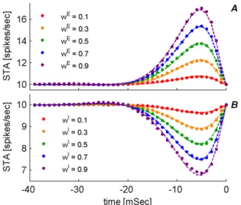
We first estimated the spike triggered average (STA) firing rate of a single presynaptic neuron triggered on postsynaptic firing, in order to approximate the function cð ÞD, equation (9). Figure 3 shows the STAs of excitatory (A) and inhibitory (B) synapses for varying levels of synaptic weights (color coded), as were estimated numerically (dots). The dashed lines show smooth curve fits to the STA. The specifictemporalstructure of these curves depends upon
particular details of the neuronal model. Nevertheless, the linear dependence on the synaptic weight is generic for weak synapses; thus, in line with the assumed linearity of the model, equation (9). The STA shows the conditional mean firing rate of the pre-synaptic neuron, given that the post fired at timet~0. In the limit of weak coupling, w?0, pre and post firing are statistically independent and the conditional mean equals the mean firing rate of the pre, rpre~10spikes=s. For an excitatory synapse, as the synaptic weight is increased the probability of a post spike following pre will also increase. Consequently, so will the likelihood of finding a pre spike during a certain time interval preceding a post spike. Hence, the STA of an excitatory synapse is expected to show higher amplitude for stronger synapse (as shown in A). Correspondingly, the STA of an inhibitory synapse is expected to show a more negative amplitude for stronger synapse (as shown inB).
To fit the STA with an analytic function we used cð ÞD~
acsin vcDyc
e{D=tc, with the fitted parametersac,vc,y c,tcfor
both the inhibitory and excitatory cases. This ad hoc approxima-tion serves to enable the numerical integraapproxima-tion that calculates the constants Xz={ that govern equation (11) for the mean field approximation to the STDP dynamics.
All the richness of physiological details that characterize the response of the post-synaptic neuron affect the STDP dynamics only via the two constants Xz and X{. These two constants
Xz={ denote the overlap between the temporal structure of the pre-post correlations,cð ÞD, and the temporal kernel,Kz={, of the potentiation/depression kernel, respectively, Figure 4. Conse-quently, ascð ÞD, is positive for excitatory synapses and negative for inhibitory synapses – so are the constantsXz={. In addition, as the correlations in our model are causal, cð ÞD~0 fortv0, the constantXz (X{) is expected to decay to zero when the STDP kernelKz(K{) vanishes from the causal branch,h?1(h?{1). For the specific choice of parameters in our simulations, DXzD obtains its maximal value at h~1. However, one may imagine other choice of parameters in whichDXzDwill obtain its maximal value ath[ð0,1Þ. Note, from Figure 4, that the crossing of theXz andX{curves, is coincidentally almost the same for both synapse types, and is obtained at&{0:2. The significance of this point is discussed below.
Fixed point solutions for the STDP dynamics
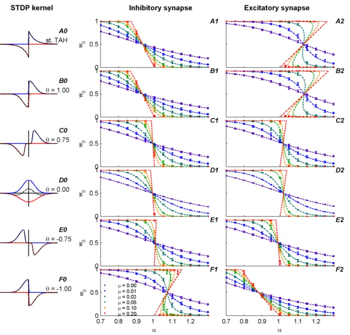
Figure 5 showsw as a function ofafor different values ofm (color coded, note that a and m are the parameters that characterize the synaptic weight dependence of the STDP rule, equations (3) and (4)). The panels depict different STDP setups that differ in terms of the temporal kernels as well as the type of synapse (excitatory/inhibitory). These two factors affect the mean field equations viaXz={. The dashed lines show the solution to the fixed point equation, equation (12), using the numerically calculated Xz={. The fixed points were also estimated numeri-cally by directly simulating the STDP dynamics in a conductance based integrate and fire neuron (circles and error bars).
numerical simulation (regression coefficient of 1+5:10{4 with R2w0:999 when performing a regression test on the entire set {w0,w} presented in each of the panels).
The panels of Figures 5A and 5B compare the standard exponential TAH rule of equation (2), in A, and our current STDP model with h~1 in B, for a representative set of parameters {(ai,mj)} applied to the examined synapse (middle column for inhibitory synapse and right column for excitatory synapse). Note that some lines may overlap each other near the boundaries:w0~0,1. As is evident from the figures, the results of the two models coincide. In particular, the Hebbian STDP dynamics of inhibitory synapses is characterized by a one to one functionw ofaand there is no bi-stability, as previously reported [13,14]. On the other hand, the Hebbian STDP of excitatory synapses is characterized by bi-stable solutions at low levels of m below a certain critical value, see e.g., [6,7]. Thus, the current model with h~1 coincides with previous results.
The panels of Figure 5F show the results of a temporally asymmetricAnti-Hebbian STDP withh~{1. In striking contrast to the Hebbian STDP, in this case, inhibitory plasticity is characterized by bi-stability whereas, the excitatory plasticity is characterized by mono-stability.
The panels of Figures 5C and 5E explore two other types of asymmetric rules (Hebbian andAnti-Hebbian respectively). These results show similar behavior as 5B and 5F in terms of the classification of STDP kernels discussed in the next section.
The panels of Figure 5D show the results of the symmetric STDP withh~0– note, that the dynamics of inhibitory synapse under the symmetric STDP rule, is characterized by a one to one functionwofacorresponding to negative feedback, as previously reported [14].
Stability of the fixed point solution
The stability of the fixed point solutionwto equation (12) is determined by the sign of the partial derivative of the dynamical equation, equation (11), with respect to the synaptic weight:
LSww_T Lw w
ð Þ~lrprerpostKK {mð1{wÞm {1
1zwXz
ð Þ
h
zð1{wÞmXz{amwm{1 1ð zwX{Þ{awmX{
ð13Þ
On the other hand, examination of Figure 5 suggests that the stability of the fixed point is governed by the sign of Lw=La. Taking the logarithm and the derivative with respect toaof both sides of equation (12), one obtains:
Lw
La~
1
a
Xz
1zwXz{
X{
1zwX{{ m
1{w{ m
w
{1
ð14Þ
sign Lw
La
~sign Xz 1zwXz
{ X{
1zwX{
{ m
1{w{ m
w
ð15Þ
where the last equality holds as aw0. At the fixed point, substituting equation (12) into equation (13) one obtains: Figure 3. Spike Triggered Average (STA) of a single
presynap-tic input.The conditional mean firing rate of the presynaptic cell given that the postsynaptic cell has fired at timet~0, is plotted as function of time. (A) Excitatory synapse (B) Inhibitory synapse. Each set of dots (color coded) is the conditional mean firing rate calculated over 1000 hours of simulation time with fixed synaptic weights and presynaptic firing rates on all inputs. The different sets correspond to a different presynaptic weight (wx) on a single synapse on which the STA was measured. The respective dashed lines show the numerical fitting of the formSTA wx,D
ð Þ~rpre 1zwxcD
ð Þ
ð Þwherecð ÞD takes the revised formula:acsin vcD
yce{D=tc. For every type of synapse, i.e.,
excitatory (in A) and inhibitory (in B), the parameters describingcð ÞD, namely ac,vc,yc,tc, were chosen to minimize the least square
difference between the analytic expression and the numerical estimation of the STA. These parameters were then used to calculate Xz={.
doi:10.1371/journal.pone.0101109.g003
Figure 4. Mean field constantsXz={of equation (11) for the
excitatory and inhibitory synapses of the neuronal model used in our numerical simulations, as a function ofh. These values were calculated using numerical integration (see File S1) with Kz={ðDt;h,tÞas defined by equations (7) and (8), witht~20msecas
Figure 5. The fixed point solution (w) of equation (12) (dotted lines), is compared to the asymptotic synaptic weight (w0) (circles),
of a single synapse learning dynamics for various learning rules as defined by equation (5).Each of the panels in the middle column (for inhibitory synapse) and in the right column (for excitatory synapse) explores the weight dependent STDP component,f+ð Þw of equations (3) and (4), for representative set ofm(shown by different colors as depicted in the legend) as a function ofa. The different rows correspond to different STDP kernels,K+ð ÞDt as shown by the panels in the left column. The circles and error bars represent the mean and standard deviation of the synaptic weight (w0), calculated over the trailing 50% of each learning dynamics simulation (see Methods). The mean field constants {Xz,X{} were
numerically calculated using thecð ÞD constants estimated as in Figure 3. The dotted lines were computed by equation (12) that was calculated for 10,000 sequential values ofwin½0,1. To this end, we replacedm~0withm~10{6in order to use equation (12) to plot the dashed red line. Initial
conditions for the simulations: for the majority of the simulations we have simply usedw~0:5as initial condition for the plastic synaptic weight. In order to show the bi-stable solutions in panels (A2, B2, F1), form~0,0:01,0:02anda~1:01,1:03,. . .1:19we ran two simulations one with initial conditionw~0and another with initial conditionw~1. (A0-F0) are the STDP kernels (as in Figure 1) used in the simulations. (A1-F1) results for the inhibitory synapse simulations. (A2-F2) results for the excitatory synapse simulations.
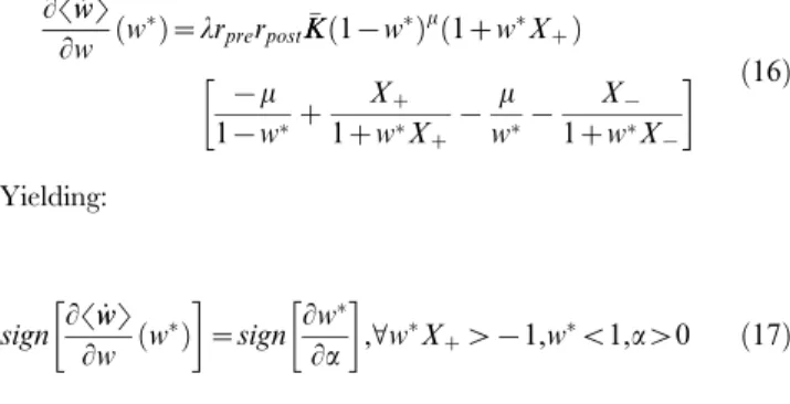
LSww_T Lw w
ð Þ~lrprerpostKKð1{wÞmð1zwXzÞ
{m
1{wz
Xz
1zwXz{ m
w{
X{
1zwX{
ð16Þ
Yielding:
sign LSww_T Lw w
ð Þ
~sign Lw La
,VwXzw{1,wv1,aw0 ð17Þ
Hence, forwXzw{1, the fixed point solution in Figure 5 is stable in segments with negative slope, and unstable in segments with positive slope. Note that in our simulation setupDXzDv1(cf. Figure 4); thus, the conditionwXzw{1holds for all values ofh in our case.
Revisiting the different scenarios depicted in Figure 5, we note the existence of two qualitatively different behaviors; namely, one that can only show mono-stability (A, C, and F) and the other has the potential for bi-stability (in panels B, D, and E). We use this behavior to classify the different STDP temporal kernels that are parameterized by the single variable h. We shall term ‘‘class-I temporal kernels’’ the temporal kernels such that w is mono-stable for all aw0;m[½0,1. We shall term ‘‘class-II temporal kernels’’ the temporal kernels such thatw is bi-stable for some m[½0,mcÞand somea mð Þ. Note that this classification depends on the type of synapse (which via cð ÞD together with h determine
Xz={). In addition, we note the existence of a special solution at
w~1=2that is invariant tom, and enables us to obtain a simple condition for this classification. In class-I kernels the derivative
Lw=Laatw~1=2is always negative, whereas in class-II models there is a critical value ofmbelow which the derivative changes its sign.
The ‘‘m-invariant’’ solution and the criticalm
Asw~1=2?ðw=ð1{wÞÞm~1Vm, the solution of the fixed
point equation, equation (12), atw~ww^:1=2ism-invariant. For a given STDP temporal kernel (h), i.e. a given set of {Xz,X{} (see Figure 4; and note thatXz={are also determined by the pre-post correlation structure viacð ÞD), the solution ofww^~1=2is obtained with:
^
a
a~1zXz=2
1zX{=2
,m[½0,1 ð18Þ
Substituting the m-invariant solution, equation (18), into equation (15), yields
sign LSww_T Lw ð^aa,ww^Þ
~
sign Xz
1zXz=2
{ X{
1zX{=2 {m 1
1=2z 1 1=2
VXzw{2 ð19Þ
Thus, the condition for instability of them-invariant solution is:
mvmc:1
4 Xz
1zXz=2
{ X{
1zX{=2
ð20Þ
Thus, for mcv0 the m-invariant solution, ww^, is stable for all values ofm[½0,1and the STDP rule is class-I for that synapse. On the other hand, if mcw0 the STDP rule is class-II. This classification depends solely on the values of {Xz,X{}. In our simulation setupDXz={Dv1(see Figure 4), thus the classification of the parameter combinations is simply determined by the sign of (Xz{X{); i.e. the manifold that is determined by the condition {Xz~X{} separates the parameter space (that characterizes the STDP rule and the synapse) between class-I and class-II.
Bimodal distribution near^aa
Figure 6 depicts (using numerical simulations with set of class-II parameters) the bifurcation plots for the learning dynamics for inhibitory (A, B) and excitatory (C, D) synapses. For inhibitory synapses the anti-Hebbian (h~{1) plasticity rules were chosen, and for the excitatory synapses, the Hebbian (h~1). The panels show the resultant distribution of the synaptic weight color-coded after 216101 of 5 hours of simulations for 21 values of the bifurcating argument (eithermora) along the abscissa. In order to calculate the synaptic weight distribution for the set of parameters without the bias of initial conditions, 101 simulations were performed with different initial weight values evenly spaced from 0 to 1. The rationale for running the simulations for 5 hours each was to make sure that the learning dynamics had reached a steady state regime and the synaptic weight fluctuated around it for the entire trailing 2.5 simulation hours. During these trailing 2.5 simulation hours, the synaptic weights were recorded at a 1 Hz sample rate. For the estimation of the weight distribution, all the samples from the 101 simulations (differing only by their initial conditions) were used with 40 evenly spread bins between 0 and 1. As expected from the analysis, there was a bifurcation along the mdimension (top panels), in which abovemc the distribution was uni-modal whereas belowmcthe distribution was bi-modal. Along the adimension (bottom panels) the distribution resembled the theoretical (dashed) curves of Figure 5 (without the unstable segment ofLw=Law0).
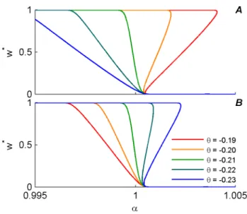
Symmetry and phase transition alongh
The high degree of similarity between the simulation results for inhibitory and excitatory synapses (Figure 5) stems from the fact that they obey the same mean-field equation (11), albeit with a different set of parameters. Thus, an excitatory synapse,wexc, with a specific choice of parameters {a,m,Xz,X{} obeys the exact same mean-field equation as (1{winh), where winh is an inhi-bitory synapse with the transformed set of parameters
1
a
:ð1zXzÞ
1zX{ ð Þ,m,
{X{
1zX{
, {Xz
1zXz
and a somewhat different
learning constant (note that Xz={ are positive for excitatory synapses and negative for inhibitory ones, see Figure 4).
synapses; i.e. for both synapses hcw{0:22 and hcv{0:21(see Figure 4). Under these conditions, for an excitatory synapse, hƒ{0:22defines the class-I kernels, andh§{0:21the class-II, whereas for an inhibitory synapse,hƒ{0:22defines the class-II kernels, andh§{0:21the class-I.
Discussion
The computational role of the temporal kernel of STDP has been studied in the past. Caˆteau and Fukai [8] provided a robust Fokker-Planck derivation and analyzed the effects of the structure of the STDP temporal kernel. However, their analysis focused on excitatory synapses and the additive learning rule (m~0). Previous studies have linked the Hebbian STDP of inhibition with negative feedback which acts as a homeostatic mechanism that balances the excitatory input to the postsynaptic cell [13,14]. Positive feedback and bi-stability of STDP dynamics have been reported only for excitation, and linked to sensitivity to the input correlation structure [6,7]. Here it was shown that the STDP of both excitation and inhibition can produce either positive or negative feedback depending on the parameters of the STDP model. Thus, for example, it was reported that both a temporally asymmetric Hebbian STDP (h~1) and a temporally symmetric learning rule (h~0) for inhibitory synapses generate negative feedback [13,14]. These reports are in-line with our finding that the criticalhfor transition from negative to positive feedback for inhibition is negative (hc&{0:2).
In general, STDP dynamics of single synapses was classified here into two distinct types. With class-I temporal kernels, the
Figure 6. Bifurcation plots along the two parameters (m=a) of the weight dependent STDP component,f+ð Þw (see equations (3) and (4)) near^aaof equation (18).Panels display the synaptic weight distribution (color coded) for the various parameter setups: (A) Inhibitory synapse with anti-Hebbian (h~{1, see also Figureoˆ 1F) rule, with fixeda~1:07and variedm. (B) Inhibitory synapse with anti-Hebbian (h~{1, see also Figureoˆ 1F) rule, with fixedm~0:025and varieda. (C) Excitatory synapse with Hebbian (h~1, see also Figureoˆ 1B) rule, with fixeda~1:13and varied m. (D) Excitatory synapse with Hebbian (h~1, see also Figureoˆ 1B) rule, with fixedm~0:05and varieda. The dashed white line marksmcin A and B, and^aain C and D.
doi:10.1371/journal.pone.0101109.g006
Figure 7. Fixed point solution,w, of the mean field
approx-imation, (plotted using equation (12)), as a function ofa, at m&0is shown for different values ofh(color coded).Usingmw0 yields continuity of the curves at the extreme values (w~1andw~0), which makes the picture clearer. On the other hand as the value ofm increases the unstable regime ofagets smaller and the resolution forh steps plotted should decrease. Thus, to plot these lines, we used m~10{4which is sufficiently close to 0 to illustrate the phase transition
dynamics is characterized by a negative feedback and has a single stable fixed point. In contrast, class-II temporal kernels are characterized by a sub-parameter regime in which the system is bi-stable (has positive feedback), and another sub-parameter regime with negative feedback. However, the mechanism that generates the negative feedback, (i.e., the stabilizing mechanism) in the two classes is different in nature. Whereas in class-I the negative feedback is governed by the convolution of the pre-post correlations with the temporal kernel, (i.e. the mean field constants
Xz={, similar to the homeostatic mechanism in [13]), in class-II, the stabilizing mechanism is the non-linear weight dependent STDP component, f+ð Þw. Hence, there is no reason a-priori to assume that the negative feedback in class-II should act as a homeostatic mechanism.
We found that there is no qualitative difference between the STDP of excitatory and inhibitory synapses and that both can exhibit class-I and class-II dynamics. Moreover, there is an exact symmetry between the excitatory and inhibitory STDP under a specific mapping of the parameters {a,m,Xz,X{}. This symmetry results from the fact that the mean-field dynamics depend solely on the global mean field constantsXz={. It is important to note that although neural dynamics is rich and diverse, due to the separation of time scales in our problem, the STDP dynamics only depends on these fine details via the global mean field constantsXz={.
Certain extensions to our work can be easily implemented into our model without altering the formalism. For example, empirical studies report different time constants for depression and potentiation, e.g. [1]. However, although in our simulations we used identical time constants atDhD~1, forDhDv1the depression time constant is larger than the potentiation time constant in our simulations. Moreover, our analytical theory depends on the time constants only viaXz={. Consequently, changing time constants or any other manipulation to the temporal kernel can be incorporated into our mean-field theory by modifying Xz={. Similarly, assuming separation of time-scales between short term and long term plasticity, the effect of short term plasticity can be incorporated by modifyingXz={accordingly.
STDP has also been reported to vary with the dendritic location, e.g. [18,25]. For a single synapse this effect can also be modeled by a modification of the parametersXz={. However, the importance of the dendritic dependence of STDP may reside in the interaction with other plastic synapses along different locations on the dendrite. Network dynamics of a ’population’ of plastic synapses is beyond the scope of the current paper and will be addressed elsewhere.
In our model we assumed that the contribution of different "STDP events" (i.e., pre-post spike pairs) to the plastic synapse are summed linearly over all pairs of pre and post spikes, see e.g. equation (21). However, empirical findings suggest that this assumption is a mere simplification, and that STDP depends on pairing frequency as well as triplets of spike time and bursts of activity, e.g. [3,26–30]. The computational implications of these and other non-linear interaction of spike pairs in the learning rule, as well as the incorporation of non-trivial temporal structure into the correlations of the pre-synaptic inputs to the cell are beyond scope of the current paper.
Empirical studies have reported a high variability of STDP temporal kernels over different brain regions, locations on the dendrite and experimental conditions, e.g., [1,12,15,17–19]. Here we represented the STDP rule as the sum of two separate processes, one for potentiation and one for depression with an additional parameter,h, that allows us to continuously modify the temporal kernel and qualitatively obtain a wide spectrum of
reported data. Representation of STDP by two processes has been suggested in the past. Graupner and Brunel [31], for example, proposed a model for synaptic plasticity in which the two processes (long term potentiation and depression) are controlled by calcium level. Thus, in their model the control parameter is a dynamical variable that may alter the plasticity rule in response to varying conditions. In our work, however, we did not model the dynamics of h. Moreover, we assumed that h remains constant during timescales that are relevant for synaptic plasticity. It is, neverthe-less, tempting to speculate on a metaplasticity process [32,33] in which the temporal structure of the STDP rule is not hard wired and can be controlled and modified by the central nervous system. Thus, in addition to controlling the learning rate,l, or the relative strength of potentiation-depression, a, a metaplasticity rule may affect the learning process by modifying the degree of ’Hebbia-nitty’,h. Such a hypothesis, if true, may account for the wide range of STDP kernels reported in the experimental literature. How can such a hypothesis be probed? One option for addressing this issue is to try and characterizehduring different time points and study its dynamics. One would expect to find that h (for excitatory synapses) decreases with time in cases where the neural network has been reported to becomes less sensitive to its input statistics, for example during developmental changes.
Methods
‘‘Mean field’’ Fokker–Planck approach for the learning dynamics
From the synaptic update rule, equation (5), changes in the synaptic weight,w, at timet, result from either pre or post synaptic firing at time t, affecting both the depression and potentiation branches (functions) of the adaptation rule. Thus:
w tðzDtÞ{w tð Þ
~lfzð ÞwP post
spike[½t,tzDt
ð
t
{?
dt0rpreð Þt0 Kzðt{t0Þ
zlfzð ÞwP pre
spike[½t,tzDt
ð
t
{?
dt0rpostð Þt0Kzðt0{tÞ
{lf{ð ÞwP post
spike[½t,tzDt
ð
t
{?
dt0rpreð Þt0 K{ðt{t0Þ
{lf{ð ÞwP pre
spike[½t,tzDt
ð
t
{?
dt0rpostð Þt0K{ðt0{tÞ ð21Þ
whererpre=postð Þt~PiD t{tprei =postis the firing of the pre/
post synaptic cell, as represented by a train of delta functions at
the neuron’s spike times, with tx
i
?
i~1 being the spike times,
andP prespike=post[½t,tzDtÞis 1 if there was a pre/post synaptic spike respectively at the specified time interval½t,tzDtÞand 0 otherwise.
Taking the short times limit, Dt?0: lim Dt?0
Pprespike=post[½t,tzDt
Dt ~
_ w
w tð Þ~lfzð ÞLw z
t
ð Þ{lf{ð ÞLw {
t
ð Þ ð22Þ
Lz={
t
ð Þ~
ðt
{?
rpreð Þt0 rpostð Þt Kz={ðt{t0Þdt’
z
ðt
{?
rpreð Þt rpostð Þt0Kz={ðt0{tÞdt’ ð23Þ
Assuming the learning process is performed on a much slower time scale than the neuronal dynamics [34], the STDP dynamics samples the pre-post correlations, rpreð Þt0rpostð Þt, over long periods in which the synaptic weight, w, is relatively constant.
Using this separation of time scales in the limit of l?0, we can approximateLz={
t
ð Þby their time average over periodT%1=l. This is the mean-field Fokker-Planck approach to approximating the stochastic dynamics of w. Integration of equation (22) over time yields: lim T?? ðT {T _ w w tð Þdt
2T ~lfzð ÞwL
z
{lf{ð ÞwL {
ð24Þ
Lz={ ~ lim T?? ð0 {? dD ðT {T dt
2TrpreðDztÞrpostð Þt Kz={ð{DÞ z ð0 {? dD ðT {T dt
2Trpreð ÞtrpostðDztÞKz={ð ÞD
Þ
ð25ÞAssuming we can replace the time averaging of the pre-post correlation with its statistical average for sufficiently largeT,
C Dð Þ:Srpreð Þ0rpostð ÞD T~ lim
T?? ðT
{T
rpreð ÞtrpostðDztÞdt 2T ð26Þ
we can substitute equation (26) into equations (25) and obtain the mean field Fokker-Planck equation for the process:
Sww_Tð Þw ~lfzð Þw
ð0
{?
Cð{DÞKzð{DÞzC Dð ÞKzð ÞD
½ dD
{lf{ð Þw
ð0
{?
Cð{DÞK{ð{DÞzC Dð ÞK{ð ÞD
½ dD
~lfzð Þw
ð?
{?
C Dð ÞKzð ÞD dD{lf{ð Þw
ð?
{?
C Dð ÞK{ð ÞDdD ð27Þ
Details of the numerical simulations
Online supporting information. This manuscript is ac-companied by a complete software package that was used throughout the study. This package is a Matlab set of scripts and utilities that includes all the numerical simulations that were used to produce the figures in this manuscript. It also contains all the scripts that generated the figures.
The leaky integrate-and-fire model. The learning dynam-ics of equation (5) was simulated by a single postsynaptic
integrate-and-fire cell. As in our previous work [13] the dynamics of the membrane potential of the postsynaptic cell,V tð Þ, obeys:
Cm
dV dt~
Vrest{V
ð Þ
Rm
zgEðEE{VÞzgIðEI{VÞ ð28Þ
whereCm~200pFis the membrane capacitance,Rm~100MVis the membrane resistance, the resting potential isVrest~{70mV, and the reversal potentials areEE~0mV andEI~{70mV. An action potential is generated once the membrane potential crosses the firing threshold Vth~{54mV, after which the membrane potential is reset to the resting potential without a refractory period. The synaptic conductances,gEandgI, are a superposition of all the synaptic contributions, i.e., each synaptic input is convolved with an a-shaped kernel (that models the filtering nature of the synaptic response) amplified by its synaptic weight and then summed. The termsgE andgIare thus given by:
gXð Þt~g0X XNX
i~1 wX
i ð Þt X
j
t{ti j
h i
z
e{ t{tij .
tX!
ð29Þ
whereXstands for Excitation or Inhibition,NXis the number of synapses, ½ tz:max t,0ð Þ is the dimensionless time value (in
seconds), and ti j
n o
j are the spike times of synapse i. For the temporal characteristic of thea-shape response we chose to use tE~tI~5ms, and for the conductance coefficient g0X our constant is scaled byNX as elaborated below.
In order to estimate the postsynaptic membrane potential in equation (28), the software performs the integration of the synaptic and leak currents using the Euler method with aDt~1msstep size. The rationale for using such a low resolution step size and its verification are discussed below.
Modeling presynaptic activity. Throughout the simula-tions in this work, presynaptic activities were modeled by an independent homogeneous Poisson processes, with stationary mean firing raterpre~10spikes=s. To this end, each of the inputs was approximated by a Bernoulli process generating binary vectors defined over discrete time bins ofDt~1ms. These vectors were then filtered using a discrete convolutiona-shaped kernel (as defined above) with a limited length of 10tX (after which this kernel function is zero for all practical purposes). In all simulations we used:NE~120,NI~40.
Conductance constants. In order to be compatible with previous studies; e.g., [7,13], and to have simulations that are executed with a robust and generic software package accompa-nying this manuscript as File S1, we scaled the synaptic conductance inversely to the number of synaptic inputs in our simulations. We used the following scaling formulag0
X~gRXSX, with: gR
E~30nS, SE~1000=NE, gRI~50nS and SI~400=NI, where NE,NI are the number of excitatory and inhibitory presynaptic inputs, respectively.
The learning rate. The simulations of the STDP process were carried out to obtain the asymptotic weight distribution of the plastic synapse. Convergence to the asymptotic region was accelerated by manipulating the learning rate constant l of equation (1). The software code was designed to support a given vector of l for each minute of the simulation. Specifically we used the following formula to generate this vector:
10{3h1z9 1ð {tÞ10i
, where t[ð0,1, is the ratio between the
10{2and decays significantly fast, leaving the trailing 70% of the simulation time with more or less the same learning rate of about
10{3.
Postsynaptic spike time accuracy vs. simulation step size resolution. Figure 5 shows the remarkable match between the fixed point solution (w) of equation (12), and the asymptotic synaptic weight (w0) of the simulations; the regression coefficient on the entire set {w0,w} in all the panels is 1+5:10{4 with R2w0:999when using an integration step of size1ms. Tests of this kind were performed on simulations using integration steps ranging from0:1msto1msin two calculation modes (see below), and it was found that higher resolution provides a better match to the analytical solution. However, the key feature that contributes to this high degree of similarity between the analysis and the simulations (more than an order of magnitude for the error term
1{R2) was the definition of the spike times of the postsynaptic cell rather than a 106decrease of the integration step size.
The spike times of an integrate and fire neuron are defined as the times in which its membrane potential crossed the firing threshold, t. However, in the numerical simulations we used discrete times,fnDtbingNn~0. In previous work we define the time of the post-synaptic firing by the last discrete time preced-ing the threshold-crossing time to: tpost~nDt such that
nDtƒtv(nz1)Dt. This choice may change the causal order of pre-post firing (from pre before post to simultaneous firing) at time
intervals of the time-bin. Consequently, it will affect the STDP rule – mainly when kernels that are discontinuous at zero are used. Here we defined the spike time of the post-synaptic neuron to be:
tpost~(nz1=2)Dt such that nDtƒtv(nz1)Dt (i.e., shifted by half a time-bin from previous definition); thus, this manipulation retains the causality of firing.
Supporting Information
File S1 This package (1Syn-STDP4PLOS.zip) is a Matlab set of scripts and utilities that includes all the numerical simulations that were used to produce the figures in this manuscript. It also contains all the scripts that generated the figures. The scripts in the main folder are divided into two categories. The files that begin with ‘‘Bat’’ execute the numerical simulations, and the ones that begin with ‘‘Plot’’ generate the figures. All the supporting numerical utilities are stored in the sub folder ‘‘CommonLib’’. (ZIP)
Author Contributions
Conceived and designed the experiments: YL MS. Performed the experiments: YL. Analyzed the data: YL MS. Contributed reagents/ materials/analysis tools: YL MS. Wrote the paper: YL MS. Designed the software used in analysis: YL.
References
1. Bi GQ, Poo MM (1998) Synaptic modifications in cultured hippocampal neurons: dependence on spike timing, synaptic strength, and postsynaptic cell type. J Neurosci 18: 10464–10472.
2. Feldman DE (2000) Timing-based LTP and LTD at vertical inputs to layer II/ III pyramidal cells in rat barrel cortex. Neuron 27: 45–56.
3. Sjostrom PJ, Turrigiano GG, Nelson SB (2001) Rate, timing, and cooperativity jointly determine cortical synaptic plasticity. Neuron 32: 1149–1164. 4. Song S, Miller KD, Abbott LF (2000) Competitive Hebbian learning through
spike-timing-dependent synaptic plasticity. Nature Neuroscience 3: 919–926. 5. van Rossum MC, Bi GQ, Turrigiano GG (2000) Stable Hebbian learning from
spike timing-dependent plasticity. J Neurosci 20: 8812–8821.
6. Rubin J, Lee DD, Sompolinsky H (2001) Equilibrium properties of temporally asymmetric Hebbian plasticity. Phys Rev Lett 86: 364–367.
7. Gutig R, Aharonov R, Rotter S, Sompolinsky H (2003) Learning input correlations through nonlinear temporally asymmetric hebbian plasticity. Journal of Neuroscience 23: 3697–3714.
8. Cateau H, Fukai T (2003) A stochastic method to predict the consequence of arbitrary forms of spike-timing-dependent plasticity. Neural Comput 15: 597– 620.
9. Gilson M, Burkitt AN, Grayden DB, Thomas DA, van Hemmen JL (2009) Emergence of network structure due to spike-timing-dependent plasticity in recurrent neuronal networks. I. Input selectivity-strengthening correlated input pathways. Biological Cybernetics 101: 81–102.
10. Morrison A, Aertsen A, Diesmann M (2007) Spike-timing-dependent plasticity in balanced random networks. Neural Comput 19: 1437–1467.
11. Standage D, Jalil S, Trappenberg T (2007) Computational consequences of experimentally derived spike-time and weight dependent plasticity rules. Biol Cybern 96: 615–623.
12. Haas JS, Nowotny T, Abarbanel HD (2006) Spike-timing-dependent plasticity of inhibitory synapses in the entorhinal cortex. J Neurophysiol 96: 3305–3313. 13. Luz Y, Shamir M (2012) Balancing feed-forward excitation and inhibition via
Hebbian inhibitory synaptic plasticity. PLoS Comput Biol 8: e1002334. 14. Vogels TP, Sprekeler H, Zenke F, Clopath C, Gerstner W (2011) Inhibitory
plasticity balances excitation and inhibition in sensory pathways and memory networks. Science 334: 1569–1573.
15. Bell CC, Han VZ, Sugawara Y, Grant K (1997) Synaptic plasticity in a cerebellum-like structure depends on temporal order. Nature 387: 278–281. 16. Nishiyama M, Hong K, Mikoshiba K, Poo MM, Kato K (2000) Calcium stores
regulate the polarity and input specificity of synaptic modification. Nature 408: 584–588.
17. Woodin MA, Ganguly K, Poo MM (2003) Coincident pre- and postsynaptic activity modifies GABAergic synapses by postsynaptic changes in Cl- transporter activity. Neuron 39: 807–820.
18. Froemke RC, Poo MM, Dan Y (2005) Spike-timing-dependent synaptic plasticity depends on dendritic location. Nature 434: 221–225.
19. Tzounopoulos T, Rubio ME, Keen JE, Trussell LO (2007) Coactivation of pre-and postsynaptic signaling mechanisms determines cell-specific spike-timing-dependent plasticity. Neuron 54: 291–301.
20. Caporale N, Dan Y (2008) Spike timing-dependent plasticity: a Hebbian learning rule. Annu Rev Neurosci 31: 25–46.
21. Vogels TP, Froemke RC, Doyon N, Gilson M, Haas JS, et al. (2013) Inhibitory synaptic plasticity: spike timing-dependence and putative network function. Front Neural Circuits 7: 119.
22. Gerstner W (2000) Population dynamics of spiking neurons: fast transients, asynchronous states, and locking. Neural Comput 12: 43–89.
23. Plesser HE, Gerstner W (2000) Noise in integrate-and-fire neurons: from stochastic input to escape rates. Neural Comput 12: 367–384.
24. Morrison A, Diesmann M, Gerstner W (2008) Phenomenological models of synaptic plasticity based on spike timing. Biol Cybern 98: 459–478. 25. Sjostrom PJ, Hausser M (2006) A cooperative switch determines the sign of
synaptic plasticity in distal dendrites of neocortical pyramidal neurons. Neuron 51: 227–238.
26. Froemke RC, Dan Y (2002) Spike-timing-dependent synaptic modification induced by natural spike trains. Nature 416: 433–438.
27. Bi GQ, Wang HX (2002) Temporal asymmetry in spike timing-dependent synaptic plasticity. Physiol Behav 77: 551–555.
28. Tzounopoulos T, Kim Y, Oertel D, Trussell LO (2004) Cell-specific, spike timing-dependent plasticities in the dorsal cochlear nucleus. Nat Neurosci 7: 719–725.
29. Wang HX, Gerkin RC, Nauen DW, Bi GQ (2005) Coactivation and timing-dependent integration of synaptic potentiation and depression. Nat Neurosci 8: 187–193.
30. Froemke RC, Tsay IA, Raad M, Long JD, Dan Y (2006) Contribution of individual spikes in burst-induced long-term synaptic modification. J Neurophysiol 95: 1620–1629.
31. Graupner M, Brunel N (2012) Calcium-based plasticity model explains sensitivity of synaptic changes to spike pattern, rate, and dendritic location. Proc Natl Acad Sci U S A 109: 3991–3996.
32. Abraham WC, Bear MF (1996) Metaplasticity: The plasticity of synaptic plasticity. Trends in Neurosciences 19: 126–130.
33. Hulme SR, Jones OD, Raymond CR, Sah P, Abraham WC (2014) Mechanisms of heterosynaptic metaplasticity. Philos Trans R Soc Lond B Biol Sci 369: 20130148.