Model
Michael Stich1*, Gourab Ghoshal1, Juan Pe´rez-Mercader1,2
1Department of Earth and Planetary Sciences, Harvard University, Cambridge, Massachusetts, United States of America,2The Santa Fe Institute, Santa Fe, New Mexico, United States of America
Abstract
We compare spot patterns generated by Turing mechanisms with those generated by replication cascades, in a model one-dimensional reaction-diffusion system. We determine the stability region of spot solutions in parameter space as a function of a natural control parameter (feed-rate) where degenerate patterns with different numbers of spots coexist for a fixed feed-rate. While it is possible to generate identical patterns via both mechanisms, we show that replication cascades lead to a wider choice of pattern profiles that can be selected through a tuning of the feed-rate, exploiting hysteresis and directionality effects of the different pattern pathways.
Citation:Stich M, Ghoshal G, Pe´rez-Mercader J (2013) Parametric Pattern Selection in a Reaction-Diffusion Model. PLoS ONE 8(10): e77337. doi:10.1371/ journal.pone.0077337
Editor:Jordi Garcia-Ojalvo, Universitat Politecnica de Catalunya, Spain
ReceivedJuly 5, 2013;AcceptedAugust 26, 2013;PublishedOctober 29, 2013
Copyright:ß2013 Stich et al. This is an open-access article distributed under the terms of the Creative Commons Attribution License, which permits unrestricted use, distribution, and reproduction in any medium, provided the original author and source are credited.
Funding:This work was carried out with support from Repsol S. A. The funders had no role in study design, data collection and analysis, decision to publish, or preparation of the manuscript.
Competing Interests:The study was supported by Repsol S. A. There are no employment, consultancy, patents, products in development and this does not alter the authors’ adherence to all the PLOS ONE policies on sharing data and materials.
* E-mail: [email protected]
Introduction
Reaction-diffusion systems are well known to self-organize into a variety of spatio-temporal patterns including, spots, stripes, spirals, as well as spatio-temporal chaos and uniform oscillations [1–3]. Their existence in out-of-equilibrium states, connection to idealized chemical systems, and dependence on dimensional parameters, make them a good testbench for the study of general features of pattern generation and evolution. In particular, the dependence of these final states on the rate at which constituents are fed into the system (feed-rate) is of significant interest, since reaction-diffusion systems represent proxies for high-level biolog-ical systems that can exchange matter and energy with the environment [4]. Depending on the value of the feed-rate, the system may asymptote into one of many states and thus the feed-rate can be thought of playing the role of a natural control parameter.
While spatio-temporal patterns in reaction-diffusion systems (like replicating spots [5] and Turing patterns [6,7]) have been found and discussed extensively in the context of chemical systems [3,8], their phenomenology is ubiquitous. A well-studied example from physics is related to electrical current filament patterns in planar gas-discharge systems [9,10]. The system dynamics can be described by activator-inhibitor reaction-diffusion models and different mechanisms of spot array formation have been observed: division and self-completion. The relevant control parameter in this system is the feeding voltage. Another example that have attracted interest recently is found in the realm of fluid dynamics where ‘‘spots’’ of turbulent regions in pipe flow [11] and plane Couette flow [12] have been observed: On a laminar background, patches of localized turbulence, called puffs, emerge via finite-amplitude perturbations and also show splitting behavior. These systems have been recently mapped onto excitable
reaction-diffusion systems [13], and subsequently, the Turing mechanism has been proposed to explain the periodic arrangement of puffs in [14], suggesting again a reaction-diffusion framework for the dynamics. The corresponding control parameter in this case is the Reynolds number of the flow.
While these examples show that similar phenomena appear in different systems, an even more intriguing feature is that patterns that
look qualitatively similar can be generated by very different
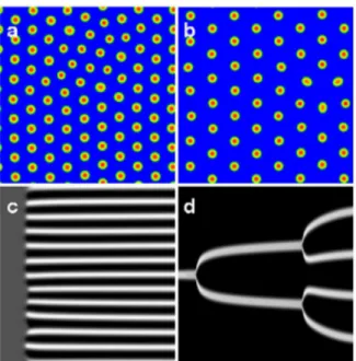
mechanisms in the same system. Consider the patterns shown in Figures 1(a,b), which are the result of numerical simulations of a typical bistable reaction-diffusion system in two spatial dimensions. While both figures represent stationary arrays of spots (increased concentrations of one or more chemical species relative to others), their evolutionary pathways are quite different. Figure 1(a) was generated by the Turing mechanism [15], i.e. from a uniform stationary state unstable under spatial perturbations, giving rise to a stationary, spatially periodic pattern. This is illustrated by a space-time diagram for a simulation in one space dimension in Fig. 1(c), where an initially uniform state almost simultaneously
developsnspots as a result of the small random perturbation.
In contrast to the above, the pattern in Fig. 1(b) was generated
by perturbing adifferentuniform steady state, creating a single spot,
that after a slight increase in the feed-rate, undergoes a replication cascade of spots, eventually filling the space (again illustrated in Fig. 1(d) by a space-time diagram for a simulation in one space dimension). Thus, while the asymptotic state of the system looks similar in both cases, the initial conditions, the parameter regimes in which they occur, and the mechanisms by which they are generated are different.
the other. If there is a coexistence region, we want to investigate whether the asymptotic states of these patterns are identical and only the temporal evolution differ. Finally, since it may be desirable to select particular states of the system we seek to
determine if it is possible to use the different mechanisms to
smoothly engineer transitions between different states.
In this article, we explore these questions in a model
reaction-diffusion system that displays both replication cascadesandTuring
instabilities. In the spirit of simplicity, tractability and clarity, we focus on a medium with only one spatial dimension and investigate
the formation of patterns as a function of the feed-rate F.
Therefore, we do not consider other pathways for the generation of spot solutions, such as transverse instabilities of stripe solutions (requiring at least two spatial dimensions). We find that, while the mechanisms driving the formation of spot arrays are discernibly
separated in different regimes of F, the patterns are essentially
indistinguishable in intermediate regimes. Nevertheless, we find degeneracies, hysteresis and directionality effects that can be exploited for the purposes of pattern selection, via the tuning of the feed-rate.
Results
The model and basic instabilities
Our model reaction-diffusion system (first introduced in [16]) is described by the differential equations
La
Lt~k1a 2b{k
2azDa
L2a
Lx2, ð1aÞ
Lb
Lt~{k1a 2b{k
3bzFzDb
L2b
Lx2, ð1bÞ
whereacan be interpreted as the concentration of an activatorA
and b as the concentration of a substrate B. There is an
autocatalytic step forAat ratek1, and decay reactions forAandB
at ratesk2,k3, whileB is fed in to the system at a rate F. The
model is closely related to a class of well-studied reaction-diffusion systems such as the Sel’kov-Gray-Scott model [17–19] (see also Sec. S1 of file S1), the Gierer-Meinhardt model [20] and the Brusselator [21].
We begin our analysis by first determining the uniform absorbing states of the model and then proceed to determine the specific instability associated with each state. Without loss of
generality, the concentrations can be rescaled to
a? ffiffiffiffiffi k1 p
a and b? ffiffiffiffiffi k1 p
b; then the stationary uniform states are
determined by setting the right-hand side of Eq. (1) to zero. Doing
so, we obtain(a1,b1)~(0,F=k3), which we refer to as state1. At a
critical value of the feed-rateFSN~2k2k31=2, we find that two more
solutions are generated by a saddle-node bifurcation. The first is anunstable intermediate state2and the second is astablestate 3
given by
(a3,b3)~((Fz
ffiffiffiffiffiffiffiffiffiffiffiffiffiffiffiffiffiffiffiffiffiffi F2{4k2
2k3 q
)=2k2,(F{
ffiffiffiffiffiffiffiffiffiffiffiffiffiffiffiffiffiffiffiffiffiffi F2{4k2
2k3 q
)=2k2). In addition to this we find that the system undergoes a Hopf
bifurcation at yet another critical value FH~k22=
ffiffiffiffiffiffiffiffiffiffiffiffiffiffi k2{k3 p
,
whereby in the rangeFSNƒFƒFH, state3is potentially unstable
with respect to temporal oscillations (for details see Sec. S2 of file S1).
Thus, the primary absorbing states of interest are 1 and 3.
These turn out to display distinct forms of instability. At a critical
feed-rate F~FT, state 3 is linearly unstable with respect to
spatially inhomogeneous perturbations, leading to the formation of
Turing patterns in the intervalFSNƒFƒFT (see Sec. S3 of file
S1). The characteristic wavelength of the pattern l can be
determined through a standard linear stability analysis, and this
determines the total number of spots n that are present in the
system through the simple relationL~nl~2pn=k, whereLis the
system size andkthe wavenumber (see Methods).
On the other hand, while state 1 is stable with respect to
infinitesimally small perturbations, it isunstableto localized
large-amplitude perturbations, that can induce the formation of a single spot. Using the technique of scale-separation, one can calculate the profiles of the spot solutions, along with the parameter regimes for
which they exist. In a particular limit, where(k3Da=k2Db)1=2%1,
we can define a critical feed-rate for the formation of single-spot
solutions, such that spots exist for
F§Fsp~2
ffiffiffi
3
p
(k2k3)3=4(Db=Da)1=4 (details are shown in Sec. S4
of file S1). As F is further increased, the single spot becomes
unstable with respect to a replication cascade (at a numerically
determined critical feed-rateFrep) which eventually fills the system
with a spot array, for related work for the Gray-Scott model see [22–30].
It is essential to point out that the fundamental difference between the formation of spot arrays via the Turing mechanism or via replication cascades, is that the former results from an
instability of state3to infinitesimally small perturbations with a
characteristic wavelength, while the latter is the result of a
localized large-amplitude perturbation to state1.
Figure 1. Stable stationary spot arrays in the reaction-diffusion system (1) generated by (a) Turing instability, (b) replication cascade. Two space dimensions are considered, with system size
Lx~Ly~100 and periodic boundary conditions. Typical formation
pathways for the Turing case (c) and the replication scenario (d) are shown in the space-time diagrams for simulations in one-dimensional space withL~150. In (a–d), the variableais displayed in color code: red, respectively white denote large values. Parameters: (a)F~3:00; (b)
F~2:20; (c)F~3:00, displayed time interval200, (d)F~2:49, displayed time interval3000. Other parameters as in Fig. 2. A pattern profile for both variablesaandbwill be shown in Fig. 4(b).
Turing patterns and localized spot patterns
We next investigate the differences between these two pattern formation mechanisms through the aid of numerical simulations, where we initialize the system in a variety of different initial states and examine the corresponding asymptotic states. To compare the generated patterns, we need to choose a suitable metric to distinguish them. In principle, there are many quantities one can measure, however, as Fig. 1 suggests, a particularly simple choice
would be to simply count the number of spotsnthat are generated
in the asymptotic state of the evolution of the system.
Consider the plot in Fig. 2, where we show the number of spots
nas a function of the feed-rateF in the asymptotic state of the
simulation (for the numerical details of the simulations, see Methods). We start with a single spot induced on the background
of state 1 in the region F§Fsp (that supports stable spots) and
gradually increase F in small increments of DF. Doing so, we
eventually reach a criticalFrepwhere the spot splits into two spots
(replicates). The 2-spot solution may again be unstable, and the splitting process is repeated. This is the situation if we start with a singlespot as initial condition. However, in the regionF§Fsp, we
can also directly create a n-spot array with nw1 by inducing
multiple large amplitude perturbations in different spatial locations of the system. The size of each spot of course is finite (being
determined by the diffusion coefficients Da,b) and consequently
there is a maximum number of spotsnmaxthat can be supported in
a finite medium. Thus in the regionFspƒFƒFrepwe can initialize
a wide range of spot arrays within the bounds1ƒnƒnmaxand by
the same procedure of incrementingF, determine the values ofF
at which the spot array replicates. The resulting curve is displayed in Fig. 2 as the lower boundary of the stability area. These values
ofF for eachnrepresent a generalization of the critical feed-rate
Frepfornw1. Clearly, this also implies that the curve corresponds
to theminimumnumber of stable spotsnmin that can be supported
by the system for fixed FwFrep, and we thus label this curve
nmin(F).
We next turn our attention to the Turing regime (FSNƒFƒFT)
and the spot patterns found there. The onset of the Turing instability is of special interest: by inducing a small-amplitude
perturbation around state3atF~FT, we obtain anativeTuring
pattern ofnT~22spots (denoted in Fig. 2 with a black square) in
very good agreement with the theoretical value predicted by linear stability analysis (see Sec. S3 and Eq. (S9) of file S1). Away from
FT, the analysis provides us with a continuousbandof unstable
wavelengths. Extensive simulations show that in the entire Turing
regime (FSNƒFƒFT), small random perturbations of state3lead
on averageto a spot pattern withnTspots (marked by the solid curve
extending fromnT~22atF~FTin Fig. 2), as predicted by linear
stability analysis using the most unstable wavelength. This is in
agreement with similar findings for the Gray-Scott model [31], confirming that patterns in this regime and initialized in this way are indeed bonafide Turing patterns.
Comparing the replication mechanism with the Turing mechanism, we recognize that the former provides an elegant
way to access a number of spots that are differentfrom nT (the
native Turing pattern)within the Turing regime. This is done by
first initializing a n-spot pattern for FspƒFƒFSN (outside the
Turing regime), and then gradually increasing F until we are
within the Turing regime. In this way we can select a wide range
of nwithin the bounds nminƒnƒnmax that differ from nT. We
note that Turing patterns withn=nT can also be generated by
expanding fronts generated by perturbing state1 in the Turing
regime (see Sec. S5 of file S1), however this is not the focus of this article.
Furthermore, starting from any stablen-spot array, we are free
to reverse the procedure anddecreaseF in increments ofDF. We
find that after a particular value ofFis reached,nnowdecreases. By
continuing this process and repeating it for all n, we obtain the
upper curve in Fig. 2 that gives themaximumnumber of stable spots
nmaxthat can be sustained for a givenF. The area enclosed by the
curves nmin and nmax thus marks the stability region of n-spot
arrays as a function of the feed-rateF. We immediately see from
the figure that degeneraten-spot arrays exist for a large range ofF,
where the arrays can in principle be generated by different
mechanisms.
Taken together, these results allow us to interpret nmax as a
disappearanceboundary where anspot solution goes to a new value
n’vn, andnmin as asplittingboundary wheren’wn. In general, in
an infinite system,nspots split into 2nspots, however in a finite
system this is constrained by its size. Therefore even in the region
that supports replication, for large enoughn, some of the spots in
the array splits while other do not. The specific value of n’ is
sensitive to small perturbations, in particular at the moment the splitting or disappearance takes place.
Clearly, as we can create many different initial conditions, many different splitting or disappearance pathways exist. As an illustrative example we show one where a single spot is initialized
on the background of state1. By increasingF, the solution reaches
the boundarynminand splitting ocurrs. The resulting two spots are
also unstable, and finally an 8-spot array is formed. By further
increasing F, the array splits into 16 spots. Then it maintains
stability for a wide range asF is increased further, well into the
Turing regime, until it splits as it encounters nmin again. This
evolution is shown via the red path in Fig. 3(a). If we now decrease
F, the boundarynmaxis encountered twice, and finally the number
of spots decreases to 1 again (shown as a blue path in Fig. 3(a)). This is an example of a hysteresis curve connected to the
degeneracy of then-spot arrays.
Another example is shown by the green path in Fig. 3(a), where we cycle the spot-array solution between 10 and 20 spots. To illustrate how this cycle lookes in a real simulation, in Fig. 3(b) we
show a space-time diagram for the variableaalong the green path.
We start from a 10-spot solution forF~2:60, increaseF in small
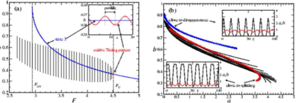
Figure 2. Stability area forn-spot arrays as a function ofFfor a system size L~200 with periodic boundary conditions and k2~1:3,k3~1:5,Da~1,Db~50(details of simulation are covered in Methods).The stability area is enclosed by the curvesnmaxandnmin,
corresponding to the maximum and minimum number of stable spots for a given F. F is changed in steps of DF~+0:05 using the asymptotic state of the previousFas initial condition (ramping). Turing patterns are marked by the curvenT. Vertical lines correspond to the
values for the instabilities:Fsp~1:90,Frep~2:45,FSN~2:94,FT~4:51.
steps until splitting to a 20-spot solution is observed. Then, we
decreaseF while preserving the 20-spot solution (hysteresis) until
finally disappearance of spots takes place and the 10-spot solution is recovered.
The hysteresis effect clearly has the consequence of a preferred directionality in the system for inducing a replication pathway.
Replication cascades proceed only via anincreasein the feed-rate
and for FrepƒFƒFT. Conversely, the formation of a Turing
pattern appears for afixedFSNƒFƒFT and for a particular class
of initial conditions.
Pattern profiles ofn-spot solutions
While measuringnhas been fruitful in determining the stability
region of the solutions, it does not provide any detailed information about the spatial distribution of the pattern. Do the spot arrays created by Turing instability and spot arrays created by
replications show any differences? Clearly, as one changes F
smoothly, the distribution of the concentration will vary, even asn
remains constant. A simple way of determining this is to measure the profile of the spots, which is the spatial range between its maximum and minimum concentrations. A visual illustration of this definition is provided in Fig. 4(a) inset.
To investigate this, we initialize a pattern withnT~22spots at
the Turing boundaryFT and examine the change in profile as we
decreaseF. In Fig. 4(a), we plot the profile ofbin function ofF. In
the same figure we mark the existence region of state 3 by the
dashed vertical boundaryFSN as well as the steady-state valueb3
by a solid blue curve (note that state3exists only forFwFSN). We
find that close toFT the amplitude of the pattern (marked by the
vertical solid lines) is small, and the concentration of boscillates
symmetrically around state3, in line with what is expected atFT
(see inset). However, as we move away from FT, the amplitude
increases and the profile shifts in phase space. At some point the
pattern ceases to oscillate around state3, and eventually decouples
from state3, continuing to persist evenbelowFSN. This decoupling
occurs without any qualitative change as the pattern crosses the
boundary. The implication of this is that forFvFSNthe persistent
spot pattern can be interpreted as a continuation of a Turing
pattern, although it is independent of state 3 (unlike a
near-threshold Turing pattern) and no Turing analysis can be applied.
In fact, spot arrays with samen, but created either through the
Turing mechanism or replication cascades show no quantitative or qualitative difference, implying that arrays created by the two mechanisms are practically indistinguishable in the intermediate regime.
We next examine the change in profile as we varyF between
the stability boundariesnmax andnmin, for an array with n~14
spots (note that for the 22-spot solution we do not reach thenmin
curve). In Fig. 4(b) we represent the resulting patterns in the space
of the concentrations(a,b). Again we see that the patterns change
continuously asFis varied, from the blue curve forF~2:1to the
red curve forF~3:42. For the former, a spatial plot of the pattern
(inset upper right) reveals that it is sharply peaked and that a spot has a small extension. If one perturbs the system by further
decreasingF by a small amount, the number of spots decreases.
Turning our attention to the other boundarynmax, an examination
of the profiles there reveals the existence of degenerate values ofa
for fixedb(marked in red). This implies that within the spot, a
small dip in the center is formed, as visualized in the inset (lower
left). Now, as one increasesFby a small amount, the spot pattern
eventually splits along this dip.
Discussion
In conclusion, using a simple reaction-diffusion model, we have
identified the stability region forn-spot solutions in the parameter
space spanned by a natural control parameter (the feed-rateF). In
general, for a givenF, we find multistability of spot solutions, with
a range of spot numbersn, bounded by numerically determined
curvesnmin andnmax.
Spot arrays in the reaction-diffusion system (1) can be created in very different ways, with two distinct limiting behaviors (single-spot solution and native Turing pattern). These arrays are
indistin-guishable in intermediate regimes (the asymptotic states for fixedF
and nare identical) where both generative mechanisms coexist.
This means that either mechanism can be used to generate the same pattern. Therefore, to discriminate between the pattern formation mechanisms is to some degree artificial, as these can only be distinguished during their transient phases. However, due to the different transients in each case, the initial conditions determine the pattern evolution and the final number of spots in a non-trivial manner: While small random perturbations create
typical Turing patterns with n coinciding on average with nT,
through an appropriate tuning ofF, we gain access to a wider
range ofnvia replication cascades. As we have shown, one can
make use of the hysteresis feature of the system to generate periodic cycles of spot replication and destruction.
Despite the simple and specific chemical nature of our model, we expect the qualitative result to hold for similar non-chemical systems and in general for those complex scenarios whose dynamics (possibly in reduced form) can by described by reaction-diffusion models such as certain fluid systems [11–14]. There, cycles of spot replication and destruction could be used to engineer transitions between out-of-equilibrium states. For exam-Figure 3. Different pattern pathways. (a) The red and blue
pathways represent a hysteresis curve for an example n-spot array induced in state 1. We observe a sequence 1?8?16?20?10?1 spots. The green path represents a cycle between 10 and 20 spots (more see text). (b) Space-time diagram fora along the green path shown in (a).F is changed aboutDF~0:05eachDt~100. Simulation starts with a 10-spot solution att~0withF~2:60, andF increases untilF~2:80, where splitting is observed. ThenF is decreased until
F~2:45, where 10 spots disappear, and after which it is increased again untilF~2:60is reached.
ple, splitting of turbulent stripes is dominant for large Reynolds numbers in plane Couette flow, while for low Reynolds numbers stripe decay is favored [12]. While the specifics in that system are different from our model, analogous to the role played by the feed-rate, we hypothesize that it could be possible to control the number of stripes through switching of the Reynolds number.
As perspectives for future work we mention the possibility to engineer the system by modulating the feed-rate in time, using a
self-generated signal (feedback) that can use the
splitting/disappear-ance pathways [32]. Furthermore, transitions between spot arrays
with different n can be also induced by application of noise.
However, the realization of these ideas goes beyond the scope of this article.
In the spirit of simplicity, tractability and clarity, we have focused on a medium with one spatial dimension. Obviously, the dynamics of localized spots and Turing patterns is much richer in two space dimensions. However, we expect that that the main result of this study holds qualitatively also for two-dimensional spot arrays.
Methods
The numerical simulations of Eq. (1) were conducted in a
one-dimensional space of size L~200 with periodic boundary
conditions which ensures that there no spots attached to the
boundary (varyingLas well as using no-flux boundary conditions
have not shown to produce mayor changes). A spatial grid with
Dx~0:5was used along with a Euler routine for time integration
and a 3-point stencil for the diffusion operator. In order for increased accuracy for patterns close to instabilities and for validation purposes, a 4th-order Runge-Kutta scheme was
employed along with a smaller grid resolutionDx~0:4and a
5-point stencil. The two-dimensional simulations shown in Fig. 1(a,b) are only for the purpose of illustration; they correspond to
simulations with Dx~Dy~0:5 and a 5-point stencil for the
diffusion operator.
We are not interested in oscillatory behavior and therefore
choose k2~1:2 and k3~1:5in order to be far from the Hopf
bifurcation curve (compare Fig. S1 of file S1). In order to observe localized spot and Turing patterns, sufficiently strong substrate
diffusion is necessary, and we setDa~1andDb~50accordingly.
Although for one-dimensional localized patterns, the notationspike
is used in the literature, we apply the more general notationspots.
To obtain the limiting curves in Fig. 2, spot solutions are
initialized for differentnin the regionFvFSN. The asymptotic
state of a simulation is determined at T~2000, although
transients usually have died out afterT&102(ifnchanges within
the simulation) or T&101 (if n does not change within the
simulation). Following this,F is increased in increments of0:05,
and the simulation is allowed to run again until the asymptotic state is reached. This procedure is repeated until splitting is
observed. In the same way,F can be either increased further or
decreased until spots split again or disappear. This iterative process
has been exhaustively performed for all possiblento determine the
stability area.
We note that the numerical results come with inherent
imprecisions, in particular for large F where the amplitude of
the Turing pattern vanishes and for smallFwhere the spot pattern
disappears. Finite simulation time may mistake a transient for an asymptotic state. Also, the finite size of the medium (together with
the periodic boundary conditions) implies that the range of n
(which is a positive integer number) is limited. However, simulations for larger system size and no-flux boundary conditions
have not revealed qualitatively new behavior, though of coursen
increases and the curves in Fig. 2 are extensive in system size.
Supporting Information
File S1. (PDF)
Author Contributions
Conceived and designed the experiments: MS GG JPM. Performed the experiments: MS GG. Analyzed the data: MS GG JPM. Contributed reagents/materials/analysis tools: MS GG. Wrote the paper: MS GG JPM.
References
1. Cross M, Greenside H (2009) Pattern Formation and Dynamics in Nonequi-librium Systems. Cambridge: Cambridge Univ. Press.
2. Mikhailov AS (1994) Foundations of Synergetics I. Berlin: Springer, 2 edition. 3. Walgraef D (1997) Spatio-Temporal Pattern Formation. New York: Springer. 4. Grzybowski BA (2009) Chemistry in Motion: Reaction-Diffusion Systems for
Micro- and Nanotechnology. Chichester: Wiley.
5. Lee KJ, McCormick WD, Pearson JE, Swinney HL (1994) Experimental observation of self- replicating spots in a reaction-diffusion system. Nature 369: 215–218.
6. Castets V, Dulos E, Boissonade J, De Kepper P (1990) Experimental evidence of a sustained standing Turing-type nonequilibrium chemical pattern. Phys Rev Lett 64: 2953–2956.
Figure 4. Pattern profiles.(a) The profile ofbin a Turing pattern as a function ofFfor fixedn~22. The blue curve represents the steady-state valueb3. The vertical dashed linesFSN andFT mark the Turing regime. A Turing pattern appears supercritically atFT(inset) and its amplitude
increases as one moves away from threshold. At a certain point, the profile ceases to oscillate aroundb3, and continues to exist beyond the Turing
regime without qualitative changes. (b) Multiple14-spot profiles in(a,b)space, forFbetweennmaxatF~2:10(blue curve) andnminatF~3:42(red curve). The insets show the corresponding concentration profiles (black isa, red isb).
7. Ouyang Q, Swinney HL (1991) Transition from a uniform state to hexagonal and striped Turing patterns. Nature 352: 610–612.
8. de Wit A (1999) Spatial patterns and spatiotemporal dynamics in chemical systems. Adv Chem Phys 109: 435–513.
9. Astrov YA, Logvin YA (1997) Formation of clusters of localized states in a gas discharge system via a self-completion scenario. Phys Rev Lett 79: 2983–2986. 10. Astrov YA, Purwins HG (2006) Spontaneous division of dissipative solitons in a planar gasdischarge system with high ohmic electrode. Phys Lett A 358: 404– 408.
11. Avila K, Moxey D, de Lozar A, Avila M, Barkley D, et al. (2011) The onset of turbulence in pipe flow. Science 333: 192–196.
12. Shi L, Avila M, Hof B (2013) Scale invariance at the onset of turbulence in Couette flow. Phys Rev Lett 110: 204502.
13. Barkley D (2011) Simplifying the complexity of pipe flow. Phys Rev E 84: 016309.
14. Manneville P (2012) Turbulent patterns in wall-bounded flows: A Turing instability? Europhys Lett 98: 64001.
15. Turing A (1952) The chemical basis of morphogenesis. Phil Trans R Soc Lond B 237: 37–72.
16. Lesmes F, Hochberg D, Mora´n F, Pe´rez-Mercader J (2003) Noise-controlled self-replicating patterns. Phys Rev Lett 91: 238301.
17. Sel’kov EE (1968) Self-oscillations in glycolysis. Europ J Biochem 4: 79–86. 18. Gray P, Scott SK (1983) Autocatalytic reactions in the isothermal, continuous
stirred tank reactor. Chem Eng Sci 38: 29–43.
19. Pearson JE (1993) Complex patterns in a simple system. Science 261: 189–192. 20. Gierer A, Meinhardt H (1972) A theory of biological pattern formation.
Kybernetik 12: 30–39.
21. Prigogine I, Lefever R (1968) Symmetry breaking instabilities in dissipative systems II. J Chem Phys 48: 1695.
22. Reynolds WN, Ponce-Dawson S, Pearson JE (1997) Self-replicating spots in reaction-diffusion systems. Phys Rev E 56: 185–198.
23. Doelman A, Kaper TJ, Zegeling PA (1997) Pattern formation in the one-dimensional Gray-Scott model. Nonlinearity 10: 523–563.
24. Nishiura Y, Ueyama D (1999) A skeleton structure of self-replicating dynamics. Physica D 130: 73–104.
25. Morgan DS, Doelman A, Kaper TJ (2000) Stationary periodic patterns in the 1D Gray-Scott model. Meth Appl Anal 7: 105–150.
26. Muratov CB, Osipov VV (2000) Static spike autosolitons in the Gray-Scott model. J Phys A Math Gen 33: 8893–8916.
27. Ei C, Nishiura Y, Ueda K (2001) 2n
-splitting or edge-splitting? Japan J Indust Appl Math 18: 181–205.
28. Muratov CB, Osipov VV (2002) Stability of the static spike autosolitons in the Gray-Scott model. SIAM J Appl Math 62: 1463–1487.
29. Kolokolnikov T, Ward MJ, Wei J (2005) The existence and stability of spike equilibria in the one-dimensional Gray-Scott model: The pulse-splitting regime. Physica D 202: 258–293.
30. Wei J, Winter M (2008) Stationary multiple spots for reaction-diffusion systems. J Math Biol 57: 53–89.
31. Mazin W, Rasmussen KE, Mosekilde E, Borckmans P, Dewel G (1996) Pattern formation in the bistable Gray-Scott model. Math Comput Simul 40: 371–396. 32. Mikhailov AS, Showalter K (2006) Control of waves, patterns and turbulence in