RESEARCH ARTICLE
lncRScan-SVM: A Tool for Predicting
Long Non-Coding RNAs Using
Support Vector Machine
Lei Sun1,2*, Hui Liu3, Lin Zhang3, Jia Meng4
1School of Information Engineering, Yangzhou University, Yangzhou, Jiangsu Province, China,2Jiangsu Co-innovation Center for Prevention and Control of Important Animal Infectious Diseases and Zoonoses, Yangzhou University, Yangzhou, Jiangsu Province, China,3School of Information and Electrical
Engineering, China University of Mining and Technology, Xuzhou, JiangSu Province, China,4Department of Biological Sciences, Xi’an Jiaotong-Liverpool University, Suzhou, Jiangsu Province, China
Abstract
Functional long non-coding RNAs (lncRNAs) have been bringing novel insight into biologi-cal study, however it is still not trivial to accurately distinguish the lncRNA transcripts (LNCTs) from the protein coding ones (PCTs). As various information and data about lncRNAs are preserved by previous studies, it is appealing to develop novel methods to identify the lncRNAs more accurately. Our method lncRScan-SVM aims at classifying PCTs and LNCTs using support vector machine (SVM). The gold-standard datasets for lncRScan-SVM model training, lncRNA prediction and method comparison were con-structed according to the GENCODE gene annotations of human and mouse respectively. By integrating features derived from gene structure, transcript sequence, potential codon sequence and conservation, lncRScan-SVM outperforms other approaches, which is evalu-ated by several criteria such as sensitivity, specificity, accuracy, Matthews correlation coef-ficient (MCC) and area under curve (AUC). In addition, several known human lncRNA datasets were assessed using lncRScan-SVM. LncRScan-SVM is an efficient tool for pre-dicting the lncRNAs, and it is quite useful for current lncRNA study.
Introduction
Recently tens of thousands of long non-coding RNAs (lncRNAs) have been discovered in the transcriptome using biotechnology such as cDNA cloning [1,2], tiling mircoarray [3–5] and high throughput sequencing [6,7]. Studies also reveal that the lncRNAs are extensively involved numerous cellular processes, such as embryonic stem cell (ESC) pluripotency, eryth-ropoiesis, cell-cycle regulation and diseases [8–11]. However, current lncRNA function studies can be hampered by lack of complete and high-quality lncRNA gene annotations, especially when conducting analysis on the genome scale. Although there appear several lncRNA data
a11111
OPEN ACCESS
Citation:Sun L, Liu H, Zhang L, Meng J (2015) lncRScan-SVM: A Tool for Predicting Long Non-Coding RNAs Using Support Vector Machine. PLoS ONE 10(10): e0139654. doi:10.1371/journal. pone.0139654
Editor:Gajendra P. S. Raghava, CSIR-Institute of Microbial Technology, INDIA
Received:March 27, 2015
Accepted:August 6, 2015
Published:October 5, 2015
Copyright:© 2015 Sun et al. This is an open access article distributed under the terms of theCreative Commons Attribution License, which permits unrestricted use, distribution, and reproduction in any medium, provided the original author and source are credited.
well-matched intersection between each other [15], which implies that the lncRNA catalogue needs to be developed. Meanwhile, with the widespread usage of deep sequencing in life sci-ence, more and more novel lncRNAs can be found due to their tissue-specific expression char-acteristic. The newly-discovered lncRNAs are always compared with previous annotations for guaranteeing the quality of further analysis [8,9].
Either for lncRNA gene annotation or novel lncRNA discovery, it is crucial to evaluate the protein coding potential of a transcript. As similar as protein-coding genes, lncRNAs are RNA polymerase II products, and can be capped and polyadenylated [16], and also present similar histone-modification profiles, splicing signals and exon/intron lengths [15]. Due to the similar-ities between mRNAs and lncRNAs, it is challenging to separate the lncRNA transcripts (LNCTs) from the protein coding ones (PCTs) [17].
Thanks to the advance of bioinformatics, discriminating LNCTs from PCTs can be mod-elled as a binary classification problem, which has been solved by several computational meth-ods, such as CONC [18], CPC [19], CNCI [20], iSeeRNA [21] and RNAcon [22]. CONC integrates various features in its classification model, but it is slow for large datasets and also performs less accurate than other newer methods such as CPC [19]. CPC uses features derived from open reading frame (ORF) and sequence alignment, and the developers also provide users with a web interface. CNCI distinguishes protein-coding and non-coding sequences by profiling adjoining nucleotide triplets, however it cannot work on large datasets. iSeeRNA out-performs previous methods and it also provides users with a program for training a new classi-fication model based on custom dataset. RNAcon applies features of tri-nucleotide
composition to the classification, but it does not show better performance than other methods in our experiment. Compared to these support vector machine (SVM) based methods inspect-ing the entire transcript, a comparative genomics method named PhyloCSF [23] focuses on classifying protein-coding and non-coding regions, and it has been frequently used for lncRNA identification [7,24]. In addition, CPAT [25] is another tool for assessing coding potential of a transcript using an alignment-free logistic regression model. Based on these computational methods, lncRNA function studies usually build a pipeline to obtain a set of confident lncRNAs [16,24,26]. For example, a simple pipeline consisting of length filtering (>200nt), CPC and BLAST [27] can make a stringent lncRNA dataset. However, it is still not convenient to master such non-standard filtering workflow.
As various information and data about lncRNAs are preserved by previous studies, it is appealing to develop new methods to identify the lncRNAs more accurately. By integrating fea-tures derived from gene structure, transcript sequence, potential codon sequence and conserva-tion, a novel computational method is proposed here for solving the problem.
Methods
Gold-standard datasets
Since a reliable dataset is of importance to model training and testing, we adopted the high-quality manually-curated GENCODE gene annotations (version 19/v19 of human and version M2/vM2 of mouse) [14,15] for constructing the gold-standard datasets, which are composed of gene annotations inGeneTransferFormat (GTF) and corresponding genome sequences in FASTA format for human and mouse respectively. Specifically, the human gene annotation (GENCODEv19) includes 81814 PCTs and 23898 LNCTs, while the counts are 47394 and 6053 respectively for mouse (GENCODEvM2). In addition, the genome sequences of human (GRCh37/hg19) and mouse (GRCm38/mm10) were downloaded from University of California Santa Cruz (UCSC) genome browser respectively [28]. For model training and testing, we cre-ated Training-A, Testing-A and Testing-B (S1 Dataset) by splitting the gold-standard datasets repository(http://hgdownload.cse.ucsc.edu/
goldenPath/hg19/chromosomes/,http://hgdownload. cse.ucsc.edu/goldenPath/mm10/chromosomes/).
Funding:This work was supported by National Natural Science Foundation of China (61301220 to LS, 61201408 to HL, 61401370 to JM),http://www. nsfc.gov.cn/; China Fundamental Research Funds for the Central Universities (2014QNA84 to HL, 2014QNB47 to LZ),http://www.moe.edu.cn/; and Jiangsu Natural Science Foundation (BK20140403 to JM),http://www.jstd.gov.cn/. The funders had no role in study design, data collection and analysis, decision to publish, or preparation of the manuscript.
(SeeTable 1). All transcripts in training and testing sets were randomly sampled from the com-plete dataset, and there are no overlapping areas between the training and testing sets. Since our prediction model was trained on Training-A, in which a proportion of transcripts may have similar sequences to that in Testing-A, which could lead to an unfair comparison between our method and the others though our method does not only use sequence features. To make a fairer comparison, Testing-B datasets were created by removing similar transcripts from Test-ing-A using CD-HIT (v4.6.1, cut-off 0.8) [29], compared to Training-A sequences. To alleviate the effect of imbalanced-classes, we constructed the training and testing sets with equal or simi-lar sizes.
Feature selection
Since each feature selected can affect the overall classification performance, we conducted fea-ture selection (FS) (SeeS1 File) based on a set of candidate features, which were derived from our current knowledge about lncRNAs. The candidate features can be classified into three cate-gories. The first category includes features extracted from nucleotide sequences, and they are 14 tri-nucleotides attributes, namely ACG, CCG, CGA, CGC, CGG, CGT, CTA, GCG, GGG, GTA, TAA, TAC, TAG and TCG [22], and standard deviation of stop codons (TAG, TAA and TGA) between three frames, and GC content. The second category was extracted from the out-put of a program calledtxCdsPredictfrom UCSC, which is used to predict a codon sequence with the most likelihood from an input nucleotide sequence, and it includes features like
txCdsPredictscore, CDS length and CDS percentage (CDS_length divided by transcrip-t_length) [21]. The third category of features was extracted from gene structure of the tran-script, and they are transcript length, exon count and average exon length.
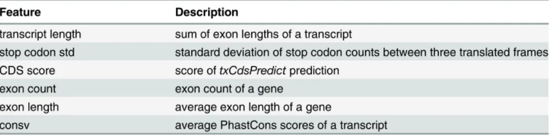
Then six features (SeeTable 2) were selected from the total candidates by FS. First, tran-script length was selected since the length of PCTs and LNCTs can be differentially distributed Table 1. Dataset partition.
Traing-A Testing set Remaining Sum
Testing-A Testing-B
human PCTs(Positive) 5000 10000 8307 66814 81814
human LNCTs(Negative) 5000 10000 8875 8898 23898
mouse PCTs(Positive) 2500 3500 3130 41394 47394
mouse LNCTs(Negative) 2500 3500 2975 53 6053
The gold-standard datasets were divided for model training and testing. Thefirst two rows show counts of divided human dataset while the other two ones show that of mouse. For human, Training-A includes 5000 PCTs randomly sampled from the totalling 81814 ones, and 5000 LNCTs sampled from the totalling 23898 ones. Human Testing-A was created by sampling another 10000 PCTs and LNCTs respectively, and human Testing-B containing 8307 PCTs and 8875 LNCTs was created by removing transcripts that show similar sequences (cutoff 0.8 of CD-HIT) to that in Training-A from Testing-A. Similarly for mouse, the counts of PCTs and LNCTs in Training-A are both 2500, and the count is 3500 in Testing-A. And counts of Testing-B for mouse PCTs and LNCTs are 3130 and 2975 respectively. Besides, the remaining transcripts (Remaining) were not taken into account in the analysis.
doi:10.1371/journal.pone.0139654.t001
three frames translated, we presume that the stop codons in the frame where the ORF emerges are fewer than that randomly appear in the other two frames. Therefore, we selected the stan-dard deviation (SCS) of stop codon counts (SCC) between three frames translated as the second feature since the standard deviation of PCT should be smaller than that of LNCT (See Eqs (1) and (2)).
x¼1 3
X 2
i¼0
SCCi ð1Þ
SCS¼ ffiffiffiffiffiffiffiffiffiffiffiffiffiffiffiffiffiffiffiffiffiffiffiffiffiffiffiffiffiffiffiffiffiffi 1 3 X 2
i¼0
ðSCCi xÞ
2 s
ð2Þ
wherexdenotes the mean of stop codon counts of three frames (SCC0,SCC1andSCC2).
ThenSCScan be calculated usingEq (2). Similarly, since the PCT may have ORF potentially, we usedtxCdsPredictto predict the codon sequence (CDS) of the candidate transcript, and the score output bytxCdsPredictwas selected as the third feature. By analysing the gene structures of transcripts, the exon count and average exon length were selected as features because the lncRNA genes may have fewer exons and be shorter than the protein-coding ones. The last fea-ture we selected is the conservation score calculated by averaging PhastCons scores of the transcript.
lncRScan-SVM
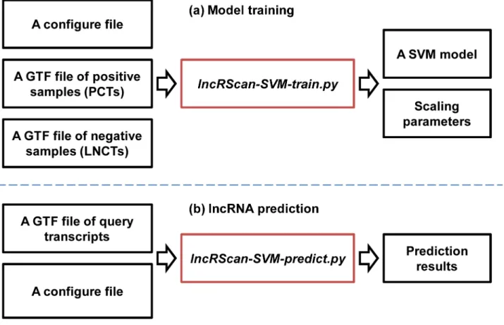
The six features selected above were fed into the SVM framework to build a tool named lncRScan-SVM (v1.0.0), which also depends on several third-part packages/programs such as BioPython [30], LIBSVM [31] andtxCdsPredict. Of the programs packaged by lncRScan-SVM, two scripts can commonly be used. One islncRScan-SVM-train.pyfor training a SVM model and the other one islncRScan-SVM-predict.pyfor predicting PCTs/LNCTs (SeeFig 1). The lncRScan-SVM package is freely available onhttp://sourceforge.net/projects/lncrscansvm/? source = directory.
Model training. A SVM model for prediction can be generated using lncRScan-SVM-train.py(SeeFig 1a). Specifically, thelncRScan-SVM-train.pyprogram first extracts nucleotide sequences according to the gene models of training samples. Then a scriptextract_features.py
is used to extract transcript features. After transferring features to a standard format of Table 2. Selected features.
Feature Description
transcript length sum of exon lengths of a transcript
stop codon std standard deviation of stop codon counts between three translated frames CDS score score oftxCdsPredictprediction
exon count exon count of a gene exon length average exon length of a gene
consv average PhastCons scores of a transcript
This table lists features of lncRScan-SVM.
LIBSVM byfeature2svm.py, a programsvm-scaleis used to scale the features. Finally, a predic-tion model can be generated.
lncRNA prediction. Users can uselncRScan-SVM-predict.pyto predict LNCTs or PCTs (SeeFig 1b). Specifically, the main input oflncRScan-SVM-predict.pyis a GTF file, which lists all transcripts for classification. Then the sequence of the query transcript is extracted using
gffread[6]. After feature extracting, formatting and scaling,svm-predictclassifies PCTs and LNCTs using the prediction model trained previously. And the prediction models for hg19 and mm10 have been packaged in lncRScan-SVM.
Evaluation
The performance of lncRScan-SVM is compared to other methods, such as CPC (v0.9-r2), CPAT (v1.2.2), iSeeRNA (v1.2.1) and RNAcon (v1.0), by several criteria, such as sensitivity (SES) or true positive rate (TPR) or recall, specificity (SPC), accuracy (ACC), Matthews Fig 1. lncRScan-SVM.(a) Model training. A GTF file of positive samples, a GTF file of negative samples and a configure file are input to lncRScan-SVM-train.pyfor training a SVM model and getting scaling parameters. (b) lncRNA prediction. A GTF file of query transcripts and a configure file are input to
lncRScan-SVM-predict.pyfor predicting PCTs or LNCTs.
doi:10.1371/journal.pone.0139654.g001
correlation coefficient (MCC).
SES¼TP
P ¼ TP
TPþFN ð3Þ
SPC¼TN
N ¼ TN
TNþFP ð4Þ
ACC¼TPþTN
PþN ð5Þ
MCC¼ ffiffiffiffiffiffiffiffiffiffiffiffiffiffiffiffiffiffiffiffiffiffiffiffiffiffiffiffiffiffiffiffiffiffiffiffiffiffiffiffiffiffiffiffiffiffiffiffiffiffiffiffiffiffiffiffiffiffiffiffiffiffiffiffiffiffiffiffiffiffiffiffiffiffiffiffiffiffiffiffiffiffiffiffiffiffiffiffiffiffiffiffiffiffiffiffiffiffiffiffiffiffiffiTPTN FPFN
ðTPþFPÞ ðTPþFNÞ ðTNþFPÞ ðTNþFNÞ
p ð6Þ
whereTP,P,TN,N,FP,FNdenote true positive, positive, true negative, negative, false posi-tive and false negaposi-tive respecposi-tively. In this paper,‘positive’and‘negative’correspond to PCT and LNCT respectively. And area under curve (AUC) of receiver operation characteristic (ROC) are also used as another indicator [32]. In addition, PhyloCSF is not took into account as it focuses on distinguishing protein-coding regions from non-coding ones, which is slightly different from the objective of the methods for classifying PCTs and LNCTs.
Ethics Statement
N/A
Results and Discussion
Performance of single feature
Since every candidate feature can contribute to the overall classification performance of a pre-dictor, the performance of each feature was evaluated by AUC scores on the hg19 and mm10 Training-A datasets respectively (SeeFig 2). As seen from the ranking result, the top eight fea-tures are CDS length, consv, CDS score, CDS percentage, exon count, stop codon std, tran-script length and CGA, which show slightly different orders between hg19 and mm10. Particularly, five of the six lncRScan-SVM features, namely transcript length, stop codon std, CDS score, exon count and consv, are included in the top eight ranked features, which indicates that most of the lncRScan-SVM features can contribute positively to the predictor. In addition, the features of hg19 and mm10 represent similar performance as seen from the the Pearson correlation coefficient (0.9484604) of the AUC scores, which shows the robustness of classifica-tion performance of the candidate features between the species.
Comparison of prediction methods
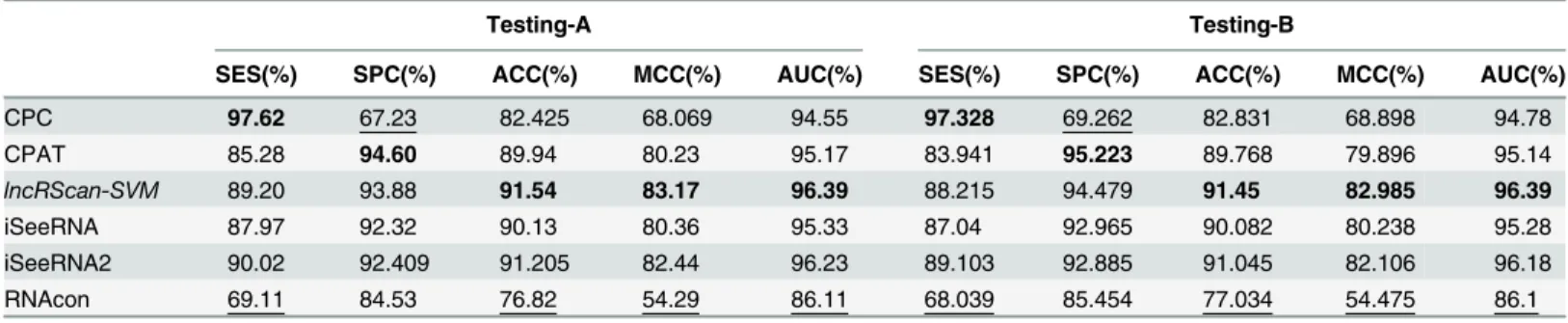
The prediction performance of lncRScan-SVM was evaluated by comparing to several other methods, such as CPC, CPAT, iSeeRNA and RNAcon, on Testing-A and Testing-B. When test-ing iSeeRNA, we used two kinds of models. One is the default iSeeRNA prediction model and the other one (iSeeRNA2) is generated by re-training iSeeRNA on Training-A. As a result, lncRScan-SVM outperforms other methods in most aspects, such as SPC, ACC, MCC and AUC (See Tables3and4).
Fig 2. Feature ranking by AUC scores.(a) The candidate features are ranked by AUC scores calculated on hg19 Training-A; (b) The candidate features are ranked by AUC scores calculated on mm10 Training-A. Each feature ID is labelled in brackets.
doi:10.1371/journal.pone.0139654.g002
Table 3. Method comparison on Testing-A and Testing-B of hg19.
Testing-A Testing-B
SES(%) SPC(%) ACC(%) MCC(%) AUC(%) SES(%) SPC(%) ACC(%) MCC(%) AUC(%)
CPC 97.62 67.23 82.425 68.069 94.55 97.328 69.262 82.831 68.898 94.78
CPAT 85.28 94.60 89.94 80.23 95.17 83.941 95.223 89.768 79.896 95.14
lncRScan-SVM 89.20 93.88 91.54 83.17 96.39 88.215 94.479 91.45 82.985 96.39
iSeeRNA 87.97 92.32 90.13 80.36 95.33 87.04 92.965 90.082 80.238 95.28
iSeeRNA2 90.02 92.409 91.205 82.44 96.23 89.103 92.885 91.045 82.106 96.18
RNAcon 69.11 84.53 76.82 54.29 86.11 68.039 85.454 77.034 54.475 86.1
CPC and CPAT were run by submitting the GTFfiles of Testing-A and Testing-B through their web interfaces. The lncRScan-SVM predictor was run after feature scaling. Besides, we tested the default iSeeRNA predictor and iSeeRNA2, an iSeeRNA model re-trained on Training-A, as well as RNAcon with a parameterTequals 0. The biggest value in each column is in bold font while the smallest one is underlined.
doi:10.1371/journal.pone.0139654.t003
most aspects. CPC obtains the highest SES (97.62% for hg19 and 98.371% for mm10), but it shows poor performance in other aspects, e.g. the lowest SPC score (67.23% for hg19 and 75.457% for mm10), which means CPC may ignore a considerable proportion of true lncRNAs. By training on Training-A, iSeeRNA2 shows better performance than the default one, but it is still less accurate than lncRScan-SVM.
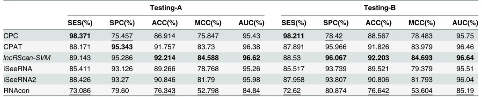
Meanwhile, similar performance of these methods can be observed from the testing result on Testing-B of hg19 and mm10, where our lncRScan-SVM predictor consistently shows better performance than other methods. As seen from the result on mm10 Testing-B (Table 4), lncRScan-SVM is ranked the highest in almost all aspects, including SPC, ACC, MCC and AUC. As indicated by SES, CPC still has a bias towards predicting PCTs, but has poor overall performance. Although the re-trained iSeeRNA2 shows similar overall performance to lncRScan-SVM, its SPC scores are much lower than the latter one, which means iSeeRNA2 would perform less accurate for identifying lncRNAs than lncRScan-SVM. In addition, the AUC scores of these methods are visualized by ROC curves (Figs3,4,5and6).
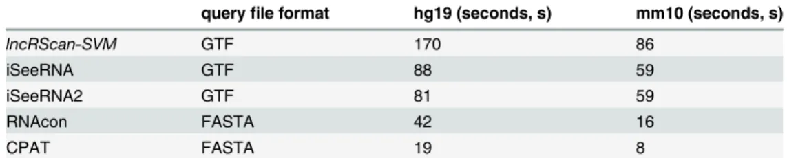
In addition to the accuracy evaluation, the computation time of these methods was also compared on the same platform (Linux, Ubuntu 12.04.4 LTS 64bit, 800 MHz × 4 processors and 4GB RAM). As seen fromTable 5, lncRScan-SVM shows the longest computation time (Nearly twice slower than iSeeRNA, four times slower than RNAcon and ten times slower than CPAT) when conducting lncRNA prediction on Testing-A of hg19 and mm10 respectively. The computation time difference can be caused by several reasons, such as different algorithms and programming languages. As seen from the table, either of the methods with query file in FASTA, namely CPAT and RNAcon, represents shorter running time than the other ones with GTF is mainly because the latter one needs longer time to extract sequence information accord-ing to the gene annotation in GTF. CPAT is faster than RNAcon because the logistic regression model used by the former one could be faster than SVM used by RNAcon. And our lncRScan-SVM is slower than iSeeRNA is mainly because we used Python scripts to implement our method, which can be optimized and accelerated using C programming in the future. Despite of that, the computation time of current lncRScan-SVM could be acceptable since its running time for precessing thousands of transcripts is still limited in several minutes or seconds. It is worth noting that CPC was not taken into account in the comparison because it is quite slow when running on the same platform. For example, it takes about 3 minutes to process only one sequence, which is much slower than the other methods.
Table 4. Method comparison on Testing-A and Testing-B of mm10.
Testing-A Testing-B
SES(%) SPC(%) ACC(%) MCC(%) AUC(%) SES(%) SPC(%) ACC(%) MCC(%) AUC(%)
CPC 98.371 75.457 86.914 75.847 95.43 98.211 78.42 88.567 78.483 95.75
CPAT 88.171 95.343 91.757 83.73 96.38 87.891 95.966 91.826 83.979 96.46
lncRScan-SVM 89.143 95.286 92.214 84.588 96.62 88.53 96.067 92.203 84.693 96.64
iSeeRNA 85.411 93.126 89.266 78.768 95.26 85.517 93.739 89.521 79.379 95.51
iSeeRNA2 88.426 93.27 90.846 81.79 95.98 87.958 93.807 90.806 81.793 96.04
RNAcon 73.086 79.60 76.343 52.798 84.84 72.62 80.874 76.642 53.604 85.19
The description for mm10 is the same asTable 3.
Prediction on known human lncRNA datasets
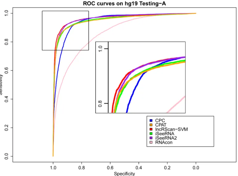
In addition to the high-quality GENCODE lncRNA dataset, previous studies have published several other lncRNA datasets, such as the NONCODEv4 dataset containing 92343 human lncRNAs [13] and the Cabili et al. dataset containing 14353 human long intergenic ncRNAs (lincRNAs) [7], which can be evaluated by lncRScan-SVM. Before conducting lncRNA predic-tion, we checked the overlap between these datasets. As seen fromFig 7plotted by eulerAPE v3 [33], the human lncRNA annotated by NONCODEv4 contains most of the lncRNAs annotated by Cabili et al. (21106,*88.32%) and GENCODEv19 (13546,*94.38%) due to the fact that NONCODEv4 published on 2014 collects a large number of ncRNAs from various literatures and databases [13]. On the other hand, the overlapping area between Cabili et al. and GENCO-DEv19 lncRNAs is small (3874,*16.36% of GENCODEv19 or*27.24% of Cabili et al.). Fig 3. ROC curves of lncRNA prediction on hg19 Testing-A.The prediction performance of CPC, CPAT, lncRScan-SVM, iSeeRNA, iSeeRNA2 and RNAcon on hg19 Testing-A is illustrated by ROC curves with colors of blue, orange, red, green, purple and pink respectively. The definitions of the sensitivity for x axis and specificity for y axis are the same as Formulas 3 and 4. The top-left area is zoomed in on for distinguishable observation.
doi:10.1371/journal.pone.0139654.g003
Then we applied lncRScan-SVM to the Cabili et al. and NONCODEv4 datasets respectively, compared with other methods (SeeTable 6). As a result, lncRScan-SVM successfully identified 14069 (98.52%) of 14281 lincRNAs annotated by Cabili et al., which were generated by a com-plex filtering pipeline mentioned in their paper [7]. On the NONCODEv4 lncRNA dataset, lncRScan-SVM successfully predicted 77435 (85.63%) of the totalling 90429 lncRNAs, which is much lower than that on the Cabili et al. dataset due to the fact that the lncRScan-SVM predic-tion model trained on GENCODEv19 that contains 12152 (50.85%) lincRNAs might have a bias towards predicting lincRNAs rather than non-intergenic lncRNAs. To test this hypothesis, we conducted lncRScan-SVM on the 43730 lincRNAs (the lncRNAs located in the intergenic regions of GENCODEv19 protein coding transcripts) extracted from the NONCODEv4 data-set. As a result, 41984 (96.01%) lincRNA were predicted successfully. Similarly, the prediction ratios of the other methods all decline as test sets change from lncRNA to lincRNA, which means they all have a bias towards predicting lincRNAs. In contrast, most of the other tools Fig 4. ROC curves of lncRNA prediction on mm10 Testing-A.The description of ROC curves for tests on mm10 Testing-A is the same asFig 3.
represent lower prediction ratios than lncRScan-SVM on the three datasets except CPAT, which has the highest prediction ratio (90.29%) on NONCODEv4 lncRNA dataset since CPAT has a bias towards predicting the lncRNAs (See previous section). However, CPAT still resents poorer performance on either Cabili et al. or NONCODEv4 lincRNAs. Overall, the pre-diction of these methods on the general lncRNA datasets is consistent with that on our gold-standard sets.
In addition, the remaining 72 lincRNAs of Cabili et al. dataset and 1964 lncRNAs or 1914 lincRNAs of NONCODEv4 were not took into account analysis because they are not annotated on the main reference chromosomes, such as chr1, chr2 and so on, but are annotated on on the other regions such as patches, scaffolds and haplotypes, and they can not be processed by sev-eral methods.
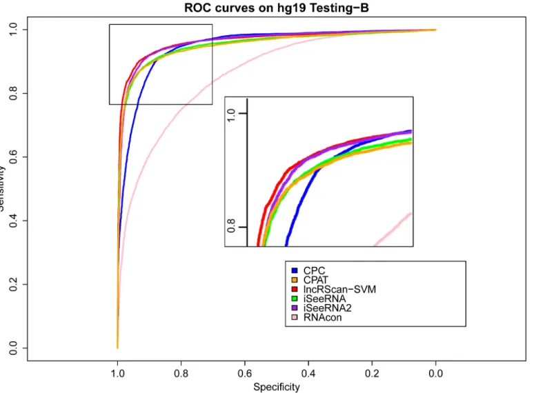
Fig 5. ROC curves of lncRNA prediction on hg19 Testing-B.The description of ROC curves for tests on hg19 Testing-B is the same asFig 3.
doi:10.1371/journal.pone.0139654.g005
Discussion
The lncRNA prediction problem can be solved by several computational methods mentioned above, especially our lncRScan-SVM performs better than the others in several aspects by inte-grating information extracted from gene structure, sequence composition and conservation in the SVM framework. However several problems remain to be specified. First, novel features and models can be developed to improve the prediction performance. For example, features can be extracted from secondary structure of RNA since functional lncRNAs may have special patterns in the secondary structure. Second, current lncRNA prediction methods present a bias towards predicting lincRNAs, so new distinguishable features should be extracted for predict-ing those non-intergenic lncRNAs, thereby helppredict-ing solve the third problem, that is a more detailed catalogue of lncRNAs needs to be created by classifying the lncRNAs into subclasses corresponding to various functions. Last but not least, it is worth noting that classifying PCTs and LNCTs might be meaningless since some lncRNAs can be bifunctional, that is some non-coding RNAs can be translated into peptides in particular circumstances [16,34].
Fig 6. ROC curves of lncRNA prediction on mm10 Testing-B.The description of ROC curves for tests on mm10 Testing-B is the same asFig 3.
Table 5. Computation time comparison on Testing-A of hg19 and mm10.
queryfile format hg19 (seconds, s) mm10 (seconds, s)
lncRScan-SVM GTF 170 86
iSeeRNA GTF 88 59
iSeeRNA2 GTF 81 59
RNAcon FASTA 42 16
CPAT FASTA 19 8
There are 20000 and 7000 samples in the Testing-A of hg19 and mm10 respectively.
doi:10.1371/journal.pone.0139654.t005
Fig 7. Overlap between three human lncRNA datasets.The lncRNA counts of the three human lncRNA datasets are proportional to the area of the ellipses. The largest ellipse denotes NONCODEv4 lncRNAs. The right-down and right-up ones are for GENCODEv19 and Cabili et al. lncRNAs respectively.
doi:10.1371/journal.pone.0139654.g007
Therefore, identifying PCTs or LNCTs is not only a simple classification problem, but also fundamental for further analysis, e.g. lncRNA function study. It is hopeful that various datasets and novel hypothesis can help improve the prediction accuracy and further deepen our under-standing of lncRNA functions.
Conclusions
Current lncRNA studies have been accelerated by various datasets and efficient bioinformatic tools. Here we proposed lncRScan-SVM, which performs better than several popular methods in predicting the lncRNAs. lncRScan-SVM is quite useful for lncRNA gene annotation and can be integrated into pipelines of lncRNA study.
Supporting Information
S1 Dataset. A compressed file containing GTF files of Training-A, A and Testing-B transcripts.
(ZIP)
S1 File. Comparison of three feature selection strategies.To select a set of good features for model training and testing, we compared three feature selection (FS) strategies.
(DOC)
Acknowledgments
The authors would like to acknowledge Dr. Lina Ma from Beijing Institute of Genomics, Chi-nese Academy of Sciences for helpful suggestions.
Author Contributions
Conceived and designed the experiments: LS. Performed the experiments: LS HL LZ JM. Ana-lyzed the data: LS. Contributed reagents/materials/analysis tools: LS. Wrote the paper: LS. Table 6. Prediction on known human lncRNA datasets.
Human lincRNA of Cabili et al. (14281 processed/14353 total)
Human lncRNA of NONCODEv4 (90429 processed/92343 total)
Human lincRNA of NONCODEv4 (43730 processed/45644 total)
lncRScan-SVM
14069 (98.52%) 77435 (85.63%) 41984 (96.01%)
iSeeRNA 13887 (97.24%) 75535 (83.53%) 41143 (94.08%)
iSeeRNA2 13848 (96.97%) 73439 (81.21%) 40821 (93.35%)
RNAcon 12651 (88.59%) 67873 (75.06%) 35431 (81.02%)
CPAT 13973 (97.84%) 81651 (90.29%) 41276 (94.39%)
CPC 10910 (76.40%) Not availablea 26380 (60.32%)
The lncRNA prediction performance of lncRScan-SVM is compared with iSeeRNA, iSeeRNA2, RNAcon, CPAT and CPC on on three human lncRNA datasets. The biggest prediction ratio is highlighted by bold font.
aCPC was not available for predicting NONCODEv4 human lncRNAs and reportedTOO_MANY_ILLEGAL_CHARACTERSafter submitting through its web server.
References
1. Okazaki Y, Furuno M, Kasukawa T, Adachi J, Bono H. Analysis of the mouse transcriptome based on functional annotation of 60,770 full-length cDNAs. Nature. 2002; 420(6915):563–573. doi:10.1038/
nature01266PMID:12466851
2. Carninci P, Kasukawa T, Katayama S, Gough J, Frith MC, Maeda N, et al. The Transcriptional Land-scape of the Mammalian Genome. Science. 2005; 309(5740):1559–1563. (Genome Network Project
Core Group). doi:10.1126/science.1112014PMID:16141072
3. Bertone P, Stolc V, Royce TE, Rozowsky JS, Urban AE, Zhu X, et al. Global Identification of Human Transcribed Sequences with Genome Tiling Arrays. Science. 2004; 306(5705):2242–2246. doi:10.
1126/science.1103388PMID:15539566
4. Guttman M, Amit I, Garber M, French C, Lin MF, Feldser D, et al. Chromatin signature reveals over a thousand highly conserved large non-coding RNAs in mammals. Nature. 2009; 458(7235):223–227.
doi:10.1038/nature07672PMID:19182780
5. Khalil AM, Guttman M, Huarte M, Garber M, Raj A, Morales DR, et al. Many human large intergenic noncoding RNAs associate with chromatin-modifying complexes and affect gene expression. Proceed-ings of the National Academy of Sciences. 2009; 106(28):11667–11672. doi:10.1073/pnas.
0904715106
6. Trapnell C, Williams BA, Pertea G, Mortazavi A, Kwan G, van Baren MJ, et al. Transcript assembly and quantification by RNA-Seq reveals unannotated transcripts and isoform switching during cell differenti-ation. Nat Biotech. 2010; 28(5):511–515. doi:10.1038/nbt.1621
7. Cabili MN, Trapnell C, Goff L, Koziol M, Tazon-Vega B, Regev A, et al. Integrative annotation of human
large intergenic noncoding RNAs reveals global properties and specific subclasses. Genes & Develop-ment. 2011; 25(18):1915–1927. doi:10.1101/gad.17446611
8. Alvarez-Dominguez JR, Hu W, Yuan B, Shi J, Park SS, Gromatzky AA, et al. Global discovery of
ery-throid long noncoding RNAs reveals novel regulators of red cell maturation. Blood. 2013; 123(4):570–
581. doi:10.1182/blood-2013-10-530683PMID:24200680
9. Sánchez Y, Segura V, Marín-Béjar O, Athie A, Marchese FP, González J, et al. Genome-wide analysis
of the human p53 transcriptional network unveils a lncRNA tumour suppressor signature. Nat Commun. 2014; 5.
10. Loewer S, Cabili MN, Guttman M, Loh YH, Thomas K, Park IH, et al. Large intergenic non-coding
RNA-RoR modulates reprogramming of human induced pluripotent stem cells. Nat Genet. 2010; 42 (12):1113–1117. doi:10.1038/ng.710PMID:21057500
11. Hung T, Wang Y, Lin MF, Koegel AK, Kotake Y, Grant GD, et al. Extensive and coordinated
transcrip-tion of noncoding RNAs within cell-cycle promoters. Nat Genet. 2011; 43(7):621–629. doi:10.1038/ng. 848PMID:21642992
12. Amaral PP, Clark MB, Gascoigne DK, Dinger ME, Mattick JS. lncRNAdb: a reference database for long
noncoding RNAs. Nucleic Acids Research. 2011; 39(suppl 1):D146–D151. doi:10.1093/nar/gkq1138 PMID:21112873
13. Xie C, Yuan J, Li H, Li M, Zhao G, Bu D, et al. NONCODEv4: exploring the world of long non-coding
RNA genes. Nucleic Acids Research. 2014; 42(D1):D98–D103. doi:10.1093/nar/gkt1222PMID: 24285305
14. Harrow J, Frankish A, Gonzalez JM, Tapanari E, Diekhans M, Kokocinski F, et al. GENCODE: The
ref-erence human genome annotation for The ENCODE Project. Genome research. 2012; 22(9):1760–
1774. doi:10.1101/gr.135350.111PMID:22955987
15. Derrien T, Johnson R, Bussotti G, Tanzer A, Djebali S, Tilgner H, et al. The GENCODE v7 catalog of human long noncoding RNAs: Analysis of their gene structure, evolution, and expression. Genome research. 2012; 22(9):1775–1789. doi:10.1101/gr.132159.111PMID:22955988
16. Ulitsky I, Bartel DP. lincRNAs: genomics, evolution, and mechanisms. Cell. 2013; 154(1):26–46. doi:
10.1016/j.cell.2013.06.020PMID:23827673
17. Clamp M, Fry B, Kamal M, Xie X, Cuff J, Lin MF, et al. Distinguishing protein-coding and noncoding genes in the human genome. Proceedings of the National Academy of Sciences. 2007; 104 (49):19428–19433. doi:10.1073/pnas.0709013104
18. Liu J, Gough J, Rost B. Distinguishing protein-coding from non-coding RNAs through support vector machines. PLoS genetics. 2006; 2(4):e29. doi:10.1371/journal.pgen.0020029PMID:16683024
19. Kong L, Zhang Y, Ye ZQ, Liu XQ, Zhao SQ, Wei L, et al. CPC: assess the protein-coding potential of transcripts using sequence features and support vector machine. Nucleic Acids Research. 2007; 35 (suppl 2):W345–W349. doi:10.1093/nar/gkm391PMID:17631615
20. Sun L, Luo H, Bu D, Zhao G, Yu K, Zhang C, et al. Utilizing sequence intrinsic composition to classify protein-coding and long non-coding transcripts. Nucleic Acids Research. 2013; 41(17):e166–e166. doi:
10.1093/nar/gkt646PMID:23892401
21. Sun K, Chen X, Jiang P, Song X, Wang H, Sun H. iSeeRNA: identification of long intergenic non-coding RNA transcripts from transcriptome sequencing data. BMC genomics. 2013; 14(Suppl 2):S7. doi:10. 1186/1471-2164-14-S2-S7PMID:23445546
22. Panwar B, Arora A, Raghava GP. Prediction and classification of ncRNAs using structural information. BMC genomics. 2014; 15(1):127. doi:10.1186/1471-2164-15-127PMID:24521294
23. Lin MF, Jungreis I, Kellis M. PhyloCSF: a comparative genomics method to distinguish protein coding and non-coding regions. Bioinformatics. 2011; 27(13):i275–i282. doi:10.1093/bioinformatics/btr209 PMID:21685081
24. Sun L, Zhang Z, Bailey T, Perkins A, Tallack M, Xu Z, et al. Prediction of novel long non-coding RNAs based on RNA-Seq data of mouse Klf1 knockout study. BMC Bioinformatics. 2012; 13(1):331. doi:10. 1186/1471-2105-13-331PMID:23237380
25. Wang L, Park HJ, Dasari S, Wang S, Kocher JP, Li W. CPAT: Coding-Potential Assessment Tool using an alignment-free logistic regression model. Nucleic Acids Research. 2013; 41(6):e74. doi:10.1093/ nar/gkt006PMID:23335781
26. Pauli A, Valen E, Lin MF, Garber M, Vastenhouw NL, Levin JZ, et al. Systematic identification of long noncoding RNAs expressed during zebrafish embryogenesis. Genome Research. 2012; 22(3):577–
591. doi:10.1101/gr.133009.111PMID:22110045
27. Altschul SF, Madden TL, Schäffer AA, Zhang J, Zhang Z, Miller W, et al. Gapped BLAST and PSI-BLAST: a new generation of protein database search programs. Nucleic Acids Research. 1997; 25 (17):3389–3402. doi:10.1093/nar/25.17.3389PMID:9254694
28. UCSC genome browser;. Available from:http://genome.ucsc.edu
29. Li W, Godzik A. Cd-hit: a fast program for clustering and comparing large sets of protein or nucleotide sequences. Bioinformatics. 2006; 22(13):1658–1659. doi:10.1093/bioinformatics/btl158PMID:
16731699
30. Cock PJA, Antao T, Chang JT, Chapman BA, Cox CJ, Dalke A, et al. Biopython: freely available Python tools for computational molecular biology and bioinformatics. Bioinformatics. 2009; 25(11):1422–1423.
doi:10.1093/bioinformatics/btp163PMID:19304878
31. Chang CC, Lin CJ. LIBSVM: A library for support vector machines. ACM Transactions on Intelligent Systems and Technology. 2011; 2:27:1–27:27. Software available athttp://www.csie.ntu.edu.tw/ *cjlin/libsvmdoi:10.1145/1961189.1961199
32. Robin X, Turck N, Hainard A, Tiberti N, Lisacek F, Sanchez JC, et al. pROC: an open-source package for R and S+ to analyze and compare ROC curves. BMC Bioinformatics. 2011; 12(1):77. doi:10.1186/ 1471-2105-12-77PMID:21414208
33. Micallef L, Rodgers P. eulerAPE: Drawing Area-proportional 3-Venn Diagrams Using Ellipses. PLoS ONE. 2014; 9(7):e101717. doi:10.1371/journal.pone.0101717PMID:25032825