Optimum Design Of On Grid Pv System Using Tracking System

50

Optimum Design Of On Grid Pv System Using

Tracking System

Abstract: The fossil fuel is a main issue in the world, due to the increase of fossil fuel cost and the depletion of the fossil fuel with continuous increasing demand on electricity. With continuous decrease of PV panels cost, it is interesting to consider generation of electricity from PV system. To provide electric energy to a load in a remote area where electric grid utility is not available or connection with grid utility is available, there are two approaches of photovoltaic system, PV without tracking system (Fixed System) and PV with tracking systems. The result shows that the energy production by using PV with tracking system generates more energy in comparison with fixed panels system. However the cost per produced KWH is less in case of using fixed panels. This is the backbone in choice between two approaches of photovoltaic system. In this work a system design and cost analysis for two approaches of photovoltaic system are considered.

Index Terms: Photovoltaic (PV) system, Tracking, ON Grid, Economics

————————————————————

1

I

Energy is basis of progress in agriculture and industry, a center of development in all fields, due to the high fuel prices and the difficulty of getting in a time of crisis, which was repeated in recent times, and power outages, due to the force of conventional energy and ending a period of not more than a century ago We went towards an alternative source, we could not find better than solar energy, Where sunlight provides by far the largest of all carbon-neutral energy sources. Sunlight strikes the Earth in one hour (4.3 × 1020 _{J) is more than all the energy consumed on the} planet in a year (4.1 × 1020 _{J), Sunlight is abundant} sources of energy in the future. It is readily available, secure from geopolitical tension, and poses no threat to our environment through pollution or to our climate through greenhouse gases. In 2001the solar electricity provided less than 0.1% of the world's electricity, and the solar fuel from modern (sustainable) biomass provided less than 1.5 % of the world's energy [9].

1.1 Solar Radiation applications

Solar energy has two main applications; thermal applications as well as photovoltaic applications. The main thermal applications are, [4], [7]:-

a) Flat-plate air collector: A device having an insulated blackened flat surface with a transparent glass window above it that works with the micro greenhouse effect. b) Solar dryer: A device that uses solar energy for drying

applications.

c) Greenhouse: A microclimate, which can be created by using the transparent glass/plastic house similar to the global greenhouse concept. It can be Used for optimum growth of living plants (e.g. flowers, vegetables, etc.) for maximum crop production during season as well as off-season (post-harvest and pre-harvest period) and is generally known as greenhouse technology. The greenhouse can also be used for crop drying for storage purposes.

d) Photovoltaic (PV device): A device used to convert short radiation into direct current (dc) electricity etc.

1.2 Sun–Earth Angles

The energy flux of beam radiation on a surface with arbitrary orientation can be obtained by the flux either on a surface perpendicular to the Sun rays or on a horizontal

surface. The various Sun–Earth angles required to understand the solar energy received are as follows [1], [3].

1.2.1 Solar Declination (�)

The angle that the Sun’s rays make with the equatorial plane is known as the declination angle (Figure 1). This angle is the solar declination. On any day, δ is taken as a constant which changes on the next day. Cooper’s empirical relation for calculating the solar declination angle (in degrees) is [1], [5], and [8]

δ= 23.45 sin 284 + n ×360

365 (1)

Where that: n = day of the year (1 ≤n≤ 365).

Fig1. Solar declination angle.

Solar declination can also be defined as the angle between the line joining the centers of the Sun and the Earth and its projection on the equatorial plane. The solar declination changes mainly due to the rotation of Earth about an axis. Its maximum value is 23.45° on 21 December and the minimum is – 23.45° on 21 June.

1.2.2 Latitude (φ) and Longitude (�_�)

51 ranging from 0° at the equator to 90° at the poles (90°N or

90°S) for the north and south poles.

Fig2. Latitude (φ) and Longitude ( ).

On the Earth, a meridian (Lt) is an imaginary north–south line between the North Pole and the South Pole that connects all locations with a given longitude. The position on the meridian is given by the latitude, each being perpendicular to all circles of latitude at the intersection points. The meridian that passes through Greenwich (England) is considered as the prime meridian, all the places on that meridian have the same longitude. The Earth can be divided in two parts with reference to the prime meridian, viz. eastern and western hemispheres. The maximum distant meridian on both sides can be at 0° to 180° from the principal meridian [1], [9], [11].

1.2.3 Hour Angle (ω)

The hour angle is the measure of the angular displacement of the Sun through which the Earth has to rotate to bring the meridian of the place directly under the Sun, At sunrise, the value of ω will be maximum, then it will slowly and steadily reduce and keep reducing with time until solar noon. At this point ω becomes zero. It starts increasing the moment after solar noon and will be maximum at sunset. The values at sunrise and sunset are numerically the same but have opposite signs. Which gives the time elapsed since the celestial body’s last transit at the observer’s meridian for a positive hour angle or the time expected for the next transit for a negative hour angle (1 hour =15°) [1],[6].[9].

Fig3. Hour angle.

1.2.4 Angle of Incidence

The angle of incidence is the angle between a beam incident on a surface and the line perpendicular to the surface. β is the inclination of the plane (a surface on which beam radiation is falling) with the horizontal surface and ƔƔ is the wall azimuth angle (due south) that specifies the orientation of the surface. This angle decides the distance of a tilted plane from the south orientation. If its value is 0° then the surface is facing towards south. If the plane under consideration is horizontal, i.e. β=0 and alsoƔƔ=0, then the angle of incidence θhbecomes equal to the zenith angle [1], [2].

1.3 Measurement of Solar Radiation on Earth’s Surface

The solar radiation reaching the Earth’s surface through the atmosphere can be classified into two components: beam (direct) and diffuse radiation [1]. Beam radiation (HD): The solar radiation propagating along the line joining the receiving surface and the Sun. It is also referred to as direct radiation. Diffuse radiation ( Hd ): The solar radiation scattered by aerosols, dust and molecules. It does not have any unique direction. Total radiation (HB): The sum of the beam and diffuse radiation, sometimes known as global radiation on horizontal surface. Solar radiation is energy received per (m2/day) and it measured always on horizontal surface it donated by HB (KWh/ m2 /day). The extraterrestrial solar irradiance (KW/m2) on surface normal to solar beams is constant and equal to solar constant GSC(=1.35 KWh/m

2

) is given by [10]

Hext = 24

πGSC[cosδcosφsinωs+ωssinδsinφ] (2)

KT= HB

Hext Clearness index (3)

1.3.1 Solar Radiation on a Horizontal Surface

The combination of both forms of solar energy (beam and diffuse) incident on a horizontal plane at the Earth’s surface is referred to as global solar energy and these three quantities (specifically their rate or irradiance) are linked mathematically as [1], [7]

HB= HDcosθZ+ Hd (4)

52 Fig 5. Solar radiation on a horizontal surface.

Direct radiation on horizontal surface HDis given by [10]

HD= 24

πGn cosδcosφsinωs+ωssinφsinδ (5)

1.3.2 Solar Radiation on an Inclined Surface

Direct radiation on tilted surface HD,t is given by [10]

HD,t= 24

πGn[ � � − � �`+�` � − � �]

(6)

Ratio between direct radiations on tilted surface to on horizontal surface Ref. [10], [14]

= ,

= � (�−�) � `+� ` (�−�) �

� � �+� � � (7)

The total radiation for any inclined (inclination = β) with any orientation of solar thermal device (for east, south, west and north)ƔƔ = – 90°, 0°, +90° and ±180° for a given latitude φ can be evaluated using the formula Ref. [10]

= [1.13 + 0.5 1 + � 1−1.13 + 0.5 (1− �)] (8)

When Reflectivity of ground ( = 0.2 for normal ground and = 0.7 for snow)

Fig6. Solar Radiations on an Inclined Surface.

Instantaneous global radiation on tilted surface defined as [10]

= 24

�− �῝

� `−� ` � ῝ (9)

1.4 Parameters of Solar Cells

1.4.1 I V Characteristics

The standard solar cell I-V characteristics is given by Eq.(10), Rs, should be small and the shunt (parallel) resistance, , should be large [1], [12], and [15].

= [ − ° (�+ )� −1 − �

+

] (10)

Fig8. I-V Characteristic for solar cell.

The short circuit current defined as [1], [11], and [12]. The array current I when V = 0

Then = … ( ≡ )

= − °(

�_�

−1) (11)

At I ≡ _�

_� = − °( �m � � −1) (12)

And at °= −� � (13)

The open circuit voltage � when I = 0 and defined as [1], [12], [15].

� = � (

°+ 1) (14)

The power delivered by the solar cell output is defined as [1]

P = − °�( � � −1) (15)

1.4.2 Maximum Power (�_���)

No power is generated under short or open circuit. The power output is defined as [1], [12], and [13].

= � × (16)

53 product IV is maximum. Thus _�is defined as [1], [12],

and [17].

_� = � _� × _� (17)

PV Standard Modules

Our design is based on 200 W, 24 V PV module and its parameters at AM1 and = 25 are � = 33 V, � _� = 25 V and = 8.27 A.

1.5 Simulation Program

MATLAB Simulation software is used to simulate the dynamic behavior of a system that is represented by a mathematical model. While the model is being simulated, the state of each part of the system is calculated at each step of the simulation using either time-based. A detailed simulation program is developed considering climatic conditions of Egypt.

Fig9. Flow chart for simulated program.

2

D

This design has been building the system and the work of the technical and economic analysis on the basis that the photovoltaic Array Production energy (110 KWh/day) in Cairo, Egypt. Total efficiency which includes the (mismatching and the inverter efficiency) = 0.85. Declination angle

δ= 23.45 sin⁡[ 284 + n ×360 365 ]

The instantaneous global radiation on tilted surface [10].

GT =

π

24 HT

cosω−cosωs῝ sinωs`−ωs`cosωs῝

Tracking instantaneous radiation on tilted surface [10].

GTracking one axis=GT × KT ( cosδ

cosθT) + (1- KT

) × GT

Tracking instantaneous radiation on tilted surface [10].

GTracking two axis=GT × KT ( 1 cosθT

) + (1- KT) × GT

Current output from PV array [11].

IA= ISC × GT−( I°× e

V Vt)

2.1 Design without Tracking (fixed panels system)

Obtain the array size for each solution at fixed Tilt angle β=30.Calculate energy production per array size using Matlab simulation program. Compare energy production cost from each solution.

Fig10. Block diagram of fixed panels system at β=30

without storage batteries and on grid.

2.2 Design with Manual Tracking

Obtain the size for each solution at Tilt angle changing every day. Calculate energy production per array size using Matlab simulation program. Compare energy production cost from each solution.

Fig11. Block diagram of Manual Tracking System without

storage batteries and on grid when Tilt angle changing

54

2.3 Design with Automatic Tracking System

2.3.1 Design with Automatic Tracking One Axis System Obtain the array size for each solution at tracking in one axis (when Latitude Angle constant and Zero Azimuth Angle Constantly ( ƔƔ = 0) .Calculate energy production per array size using Matlab simulation program. Compare energy production cost from each solution.

Figure (12) Block diagram of Automatic Tracking System

for One Axis without storage batteries and on grid when

Zero Azimuth Angle and β = φ .

2.3.2 Design with Automatic Tracking Two Axis System Obtain the array size for each solution at tracking in two axis (when subtract between Latitude Angle and declination angle changing every day and Zero Azimuth Angle Constantly (ƔƔ=0).Calculate energy production per array size using Matlab simulation program. Compare energy production cost from each solution.

Fig13. Block diagram of Automatic Tracking System for Two

Axis without storage batteries and on grid when Azimuth Angle=0 and β= (φ -�).

3

R

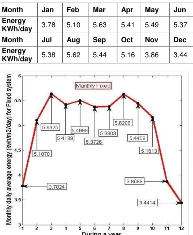
3 .1 Design without Tracking (Fixed panels System) For φ=30° (Cairo, Egypt), Tilt angle β=30°. Monthly daily average energy produced by 1 KWp array installed in Cairo (30°N) in KWh per day is shown below:-

Table 1.1 Monthly daily average energy produced by 1

KWp for fixed system.

Month Jan Feb Mar Apr May Jun

Energy

KWh/day 3.78 5.10 5.63 5.41 5.49 5.37

Month Jul Aug Sep Oct Nov Dec

Energy

KWh/day 5.38 5.62 5.44 5.16 3.86 3.44

Fig14. Monthly daily average produced by 1 KWp in Cairo

(30°N) with fixed system at �=30.

The total energy annually for system (1 KWh/ day) =1816.2 KWh/ year = 1.8162 MWh/year. For the 110 KWp

system is considered since it is standard with conventional two axis tracking. The total energy annually for system (110 KWh/day) = 199.784 MWh/year.

3.2. Design with Manual Tracking System

For φ=30° (Cairo, Egypt), the optimum tilt angle β is (φ – δ).This value makes solar beam perpendicular on PV modules at noon. Monthly daily average energy produced by 1 KWp array installed in Cairo (30°N) in KWh per day is shown below:

Table 1.2 Monthly daily average energy produced by (1

KWp) for manual tracking system.

Month Jan Feb Mar Apr May Jun

Energy

KWh/day 4.22 5.40 5.63 5.41 6.10 6.28

Month Jul Aug Sep Oct Nov Dec

Energy

55

Fig15. Monthly daily average produced by 1 KWp in Cairo

(30°N) with manual tracking at change Tilt angle every month.

The total energy annually for system ( 1 KWh/ day) =1945.5 KWh/ year =1.9455 MWh/year. The total energy annually for system (110 KWh/day) =214M Wh/year.

3 .3 Design with Automatic Tracking System

3.3.1 Design with Automatic Tracking One Axis System For φ=30° (Cairo, Egypt), β=30°. Monthly daily average energy produced by 1 KWp array installed in Cairo (30°N) in KWh per day is shown below:

Table 1.3 Monthly daily average energy produced by (1

KWp) for automatic One axis trackingsystem.

Month Jan Feb Mar Apr May Jun

Energy KWh/day

5.2

4 7.31 8.09 7.77 7.98 7.89

Month Jul Aug Sep Oct Nov Dec

Energy KWh/day

7.9

3 8.27 7.97 7.55 5.44 4.76

Fig16. Monthly daily average produced by 1 KWp in Cairo

(30°N) with One axis trackingat Ɣ =� and � = 30°.

Total energy annually for system (1 KWh/ day) = 2621.8 KWh/ year = 2.6218 MWh/year. Total energy annually for system (110 KWh/day) =288.395 MWh/year.

3.3.2 Design with Automatic Tracking Two Axis System For φ=30° (Cairo, Egypt),β= (φ - δ). Monthly daily average energy produced by 1 KWp array installed in Cairo (30°N) in KWh per day is shown below:-

Table 1.4 Monthly daily average energy produced by 1

KWp for automatic two axis trackingsystem.

Month Jan Feb Mar Apr May Jun

Energy

KWh/day 5.93 7.75 8.15 8.01 8.85 9.20

Month Jul Aug Sep Oct Nov Dec

Energy

KWh/day 9.02 8.73 8.01 7.83 6.05 5.54

Fig17. Monthly daily average produced by 1 KWp in Cairo

(30°N) with One axis trackingsystem atƔ=� and β= (φ

-�).

56

Fig18. Monthly daily average produced by 1 KWp in Cairo

(30°N) with (Fixed System, Manual Tracking System, Automatic One Axis Tracking System and Automatic Two

Axis Tracking System).

4

E

Compare between initial cost, cost (EGP) per KWh and interest rate for all system When it is implemented in Egypt and sold to the Egyptian government [16], [17].

Table1.5 Comparing between initial cost, cost (EGP) per

KWh and interest rate for each solution with all systems.

Compare Fixed System Manual Tracking System Automati c Tracking One Axis System Automatic Tracking Two Axis System Initial Cost

(EGP) 1,272,000

1,453,326

.2 2,017,975 2,255,300

W it hout Loan Cost / KWh (EGP)

0.75 0.81 0.83 0.86

Interes t rate (%)

11.50 10.60 10.10 9.70

Loan 4 % Cost / KWh (EGP)

0.73 0.78 0.80 0.83

Interes t rate (%)

19.80 18.30 17.60 14.20

Loan 1 4 % Cost / KWh (EGP)

0.88 0.94 0.97 1

Interes t rate (%)

9.89 7.56 - 1.79 1

Figure (19) compare between Cost [(EGP) / KWh] when

used payment method [without loan and loan 4% and loan 14%] for all systems.

Is the investment acceptable?

Acceptable when the Interest Rate is greater than the banking investment interest (11%) in Egypt Otherwise it is unacceptable [18], [19].

Table (6) compare between investment (acceptable or

unacceptable) for each solution with all systems.

Compare Fixed System Manual Trackin g System Automat ic Tracking One Axis System Automat ic Tracking Two Axis System W it hout L oan Interest rate (%)

11.50 10.60 10.10 9.70

State investme nt(Accept able or Unaccept able)

A U U U

Loan 4 % Interest rate (%)

19.80 18.30 17.60 14.20

State investme nt (Acceptab le or Unaccept able)

A A A A

Loan 1 4 % Interest rate (%)

9.89 7.56 - 1.79 1

State investme nt(Accept able or Unaccept able)

U U U U

0 0.2 0.4 0.6 0.8 1 1.2 Fixed System Manual Tracking System Automatic Tracking One Axis System Automatic Tracking Two Axis System

Loan 4 %

Without Loan

57

5

C

The research showed that PV system is a promising project since PV panel cost is continuing decrease in cost. This research considered comparison among PV systems (Fixed – Manual – One axis – Two axis) using on grid tracking system for producing 110 KWp. The criterion used in this research to determine the optimum solution is the cost of produced one kilo watt hour. However, it is shown that two axis automatic tracking system produces maximum energy. But PV fixed panels system is Optimum economically among PV systems, where it is less expensive to produce energy and more profitable. If exceeded energy is sold to Egyptian government (according to new laws approved by Egyptian government), according to governmental facilities approved, it is allowed borrow up to 70% of the initial cost of the project. Economic analysis showed that borrowing at 4% interest gives minimum system cost. The profit in this case return on this project is expected to be 19.8 % and also in this system total cost to produce 1 KWh is about 0.73 EGP/ KWh, It is less the cost price of production 1 KWh by conventional methods.

6

R

[1] Tiwari, Gopal Nath, and Swapnil Dubey.‖ Fundamentals of photovoltaic modules and their applications‖. No. 2. Royal Society of Chemistry, 2010.

[2] Tiwari, Gopal Nath. ―Solar energy: fundamentals, design, modelling and applications‖. Alpha Science Int'l Ltd., 2002.

[3] Anis, Wagdy R., Robert P. Mertens, and R. Van Overstraeten. "Analysis of a photovoltaic powered reverse osmosis water desalination system." Solar cells15, no. 1 ,1985

[4] Lewis, Nathan S., and George Crabtree. "Basic research needs for solar energy utilization: report of the basic energy sciences workshop on solar energy utilization, April 18-21, 2005.", 2005..

[5] Fröhlich, C., and R. W. Brusa. "Solar radiation and its variation in time."Physics of Solar Variations. Springer Netherlands, 1981. 209-215.

[6] Pluta, W. ―Solar elctricity. An economic approach to solar energy‖, 1978.

[7] Duffie, J. A., & Beckman, W. A. ―Solar engineering of thermal processes‖, (Vol. 3). New York etc.: Wiley, 1980.

[8] Cooper, P. I..―The absorption of radiation in solar stills. Solar energy‖,12(3), 333-346, 1969.

[9] D.rapp.‖ Solar Energy‖. New Jersey, 1981.

[10]Klein, S. A. ―Calculation of monthly average insolation on tilted surfaces‖. Solar energy, 19(4), 325-329, 1977.

[11]Watmuff, J. H., Charters, W. W. S., & Proctor, D. ―Solar and wind induced external coefficients-solar collectors‖. Cooperation Mediterraneenne pour l'Energie Solaire, 1, 56, (1977).

[12]Green, M. A. ―Solar cells: operating principles, technology, and system applications‖, 1982.

[13]Kumar, A., & Kandpal, T. C.― Solar drying and CO 2 emissions mitigation: potential for selected cash crops in India‖. Solar Energy, 78(2), 321-329, 2005.

[14]Linn, J. K., & Zimmerman, J. C.― Method for calculating shadows cast by two-axis tracking solar collectors ―(No. SAND-79-0190). Sandia Labs., Albuquerque, NM (USA)., 1979.

[15]Zimmerman, J. C.‖ Sun-pointing programs and their accuracy‖. NASA STI/Recon Technical Report N, 81, 30643, 1981.

[16]Sullivan, W. G., Bontadelli, J. A., & Wicks, E. M. Engineering Economy.Printice Hall, 68, 2000.

[17]Blank, L., & Tarquin, A.‖McGraw-Hill series in industrial engineering and management science. Engineering Economy‖, 2005.

[18]Samuelson, P. A., & Nordhaus, W. D. ―Economics. International Edition‖.New York. McGraw-Hill Inc, 1995.