Design Sensitivity Analysis and Optimization of McPherson Suspension Systems

(1)

Design Sensitivity Analysis and Optimization

of McPherson Suspension Systems

Hee G. Lee, Chong J. Won, and Jung W. Kim

Abstract—Design sensitivity analysis and optimization of vehicle suspension systems is presented. The design process of suspension systems consists of pre-processing design stage, analysis stage and post-processing stage. For kinematic modeling of suspension systems, McPherson strut suspension system is adopted, where suspensions are assumed as combinations of rigid bodies and ideal frictionless joints. Constraint equations for displacement, velocity and acceleration using displacement matrix method and instantaneous screw axis theorem, sensitivities of static design factor and optimum design are obtained. The validity and usefulness of the method employed are demonstrated to yield the effective suspension layout at early design stage.

Index Terms— Design sensitivity analysis, McPherson suspension, optimization,static design factor

I. INTRODUCTION

Some important characteristics of suspension systems in vehicle dynamics are mainly kinematic motions and reactions to the forces and moments transmitted from tires through chassis [1]. Design requirements for such suspension systems are to determine the design variables to meet the behavior of wheels defined through dynamic analysis and to meet the requirements for forces and moments transmitted from tires, which is very difficult for designers to determine since the suspension systems consist of different kinds of 3-dimensional mechanical elements kinematically and the behaviors are highly non-linear. In spite of the difficulties, it may be possible to design the vehicle suspension systems effectively to meet the requirements simultaneously mentioned above.

Conventional design studies of suspension systems are mainly focused on displacement and velocity. Suh [2]-[4] carried out the analyses of displacement and velocity of suspension systems using displacement matrix and the analysis of instantaneous screw axis during bump and rebound using velocity matrix. Also, he carried out the force analysis at each joint using displacement matrix and system reduction method by treating the suspension system as single mass dynamic system. Kang et al. [5] carried out the analyses of displacement, velocity and acceleration for McPherson strut suspension system using displacement matrix. Lee [6] carried out the sensitivity analysis of instantaneous screw axis through velocity analysis of multi-link suspension

system. Tak [7] obtained the dynamic optimum design through sensitivity analysis and Min [8] carried out the sensitivity analysis for kinematic static design factor using direct differentiation.

Manuscript received March 3, 2008.

H. G Lee is with Korea Military Academy, Seoul 139-799 Korea.(phone: +82-2-2197-2953; fax: +82-2-2197-0198; e-mail: hklee@ kma.ac.kr).

C. J. Won is with Kook-min University, Seoul 136-702 Korea (e-mail: cjwon@kookmin.ac.kr).

J. W. Kim is with JATCO, Seoul 153-803 Korea (e-mail:

In this paper, sensitivity analysis for kinematic static design factor determining the motion characteristics of suspension systems and sensitivity analysis and optimization for reaction at each joint are carried out with which the designers can consider the riding quality and steering stability in suspension system design and predict the change of suspension factors required depending on the vehicle characteristics. This may help the designers to determine layout of the suspension system and to develop the integrated optimum design system of suspension.

II. DESIGN PROCESS OF SUSPENSION SYSTEMS

The design optimization process of vehicle suspension systems consists of pre-processing, analysis and post-processing stages. In pre-processing stage, the suspension systems are modeled as links of kinematic elements and simple joints and also design equations for analysis are derived. In analysis stage, analyses of displacement, velocity and acceleration based on the design equations derived in pre-processing design stage, analyses of forces and moments, and analysis of static design factor of suspension systems are carried out. Finally, in post-processing design stage, design sensitivity analysis and optimization of the static design factor and reactions with respect to the design variable are carried out. Fig. 1 shows design stages integrating the entire design processes.

Product databas e

Pre-proces s ing Des ign Stage

Pre-proces s ing Des ign S tage

Ana lys is

Pos t-Proces s ing Des ign S ta ge

Pos t-Proces s ing Des ign Sta ge S us pens ion

Type

Des ign equation

Des ign Variable (Ha rd point) Cons tra int

equation

Kinematic

Sus pens ion des ion factor Sus pens ion

Modeling

Analys is

Model Verification

Optimiza tion Analys is

res ult

S ens itivity analys is

(2)

III. PRE-PROCESSING DESIGN STAGE

Pre-processing design stage is focused on modeling of suspension systems and deriving of design equations. The suspension system is modeled to enable the kinematic analysis by considering that it consists of several kinematic elements. For kinematic modeling, it is assumed that components are rigid bodies without elastic deformations for links and are ideal joints without friction or strain for joints. Design equations for displacement, velocity and acceleration constraints are derived between links of suspension systems by displacement matrix method and instantaneous screw axis theorem. McPherson strut suspension (Fig. 2) which is widely used for independent suspension system is taken for illustration.

S

coil spring

strut C

damper

wheel assembly lower arm

tie rod R S

S

Fig. 2 McPherson strut suspension

A. Kinematic modeling of suspension systems

Typical independent-type McPherson strut suspension system of Fig. 2 consists of wheel assembly connected to the tire, lower arm connecting chassis and wheel assembly, tie rod for steering and strut involving spring-damper system absorbing the shock from the road surface. Here, R, S and C represent revolute joint, spherical joint and cylindrical joint, respectively.

Since the suspension system consists of several kinematic members, each member can be modeled as links and simple joints. Fig. 3 shows the idealized model of McPherson strut suspension in which each member is connected as revolute joint at point A0 and spherical joints at points A1, B0, B1, C0, and cylindrical joint at point J1, respectively. Link A0A1 represents the lower arm connected as revolute joint with chassis and as spherical joint with wheel assembly. Link BB0B1B represents the tie rod connected as spherical joint with

chassis and wheel assembly. Also, link C0D1 represents the strut connected with spring-damper and as cylindrical joint with wheel assembly and as spherical joint with chassis. Therefore, this McPherson strut suspension can be kinematically modeled simply as in Fig. 4 and then the governing equations for each link can be derived easily. Here, McPherson strut suspension consists of Revolute-Spherical (R-S) link for lower arm modeling, Spherical-Spherical(S-S) link for tie- rod modeling and Spherical-Cylindrical(S-C) link for strut modeling.

0

A G

0

C

1 D

1 P

1

A

1

B

0

B x

y z

U

1 CD U

1 J

0

Fig. 3 Idealized model of McPherson strut suspension

S-C link

S-S link

R-S link Tie rod

Lower arm strut

0 A

1 A 0

B

1 B

0 C

1 D

1 P

Fig. 4 Kinematic modeling of McPherson strut suspension

B. Design Equations

Design equations are written as constraint equations of displacement, velocity and acceleration using displacement matrix and instantaneous screw axis depending on the joint connections between links of suspension system. Also, by corresponding actively to the change of design points due to loads from road surface, equilibrium equations for load analysis and joint design to increase the steering stability are obtained.

(3)

(a) R-S Link

- Displacement constraint equation for a new position An:

2 0 2 0 2 0 2 0 1 2 0 1 2 0 1 ) ( ) ( ) ( ) ( ) ( ) ( Z nZ Y nY X nX Z Z Y Y X X A A A A A A A A A A A A − + − + − = − + − +

− ₍₁₎

0 ) ( ) ( )

( nX − 0X + Y nY − 0Y + Z nZ − 0Z =

X A A U A A U A A

U (2)

Also, the additional constraint equation for unit vector is as follows: (3) 1 2 2

2 ₊ ₊ ₌

Z Y

X U U

U

- Velocity constraint equation:

0 ) ( ) ( )

( _nX− ₀_X + _nY _nY − ₀_Y + _nZ _nZ− ₀_Z =

nX A A A A A A A A

A (4)

0 =

+

Y nY Z nZ

nX

X

A

U

A

U

A

U

(5)

- Acceleration constraint equation:

(6) 0 ) ( ) ( ) ( 2 0 2 0 2

0 + + − + + − + =

− X nX nY nY Y nY nZ nZ Z nZ nX

nXA A A A A A A A A A A

A

0 =

+

Y nY Z nZ

nX

X

A

U

A

U

A

U

(7)

(b) S-S Link

- Displacement constraint equation for a new position Bn:

2 0 2 0 2 0 2 0 1 2 0 1 2 0 1 ) ( ) ( ) ( ) ( ) ( ) ( Z nZ Y nY X nX Z Z Y Y X X B B B B B B B B B B B B − + − + − = − + − + − (8)

- Velocity constraint equation:

0 ) ( ) ( )

( nX − 0X + nY nY− 0Y + nZ nZ− 0Z =

nX B B B B B B B B

B (9)

- Acceleration constraint equation:

0 ) ( ) ( )

( 0 2

2 0 2

0 + + − + + − + =

− X nX nY nY Y nY nZ nZ Z nZ nX

nXB B B B B B B B B B B

B (10)

Similarly, constraint equations(displacement, velocity and acceleration) for S-C Link can be obtained.

Equilibrium equations at each member can be obtained. The equilibrium equations for member A (lower arm) are written as follows:

0

1

0

+

A

−

A m

=

A

F

m

A

F

(x,y,z components) (11)

0

1

0

+

A

+

A

−

A

=

A

T

M

H

T

(x,z components) (12)

where

H

represents change rate of angular momentum. Similarly, equilibrium equations for members B (tie rod), C(strut) and E(wheel assembly) can be obtained yielding 21 equations together with (11) and (12), with which reaction and moment at each joint are obtained.

IV. ANALYSIS

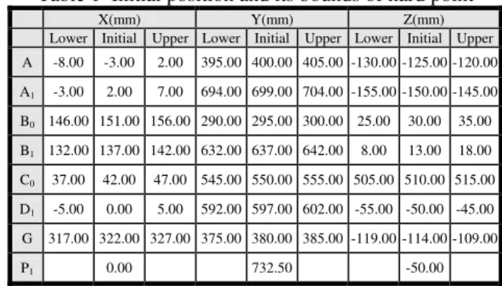
In analysis stage, the analyses for static design factor of suspension system for displacement, velocity and acceleration and for forces and moments are carried out for the McPherson strut suspension model of Fig. 3. The initial position and its bounds(lower and upper) of hard point(design variable) are as in Table 1.

Table 1 Initial position and its bounds of hard point X(mm) Y(mm) Z(mm) Lower Initial Upper Lower Initial Upper Lower Initial Upper A -8.00 -3.00 2.00 395.00 400.00 405.00 -130.00 -125.00 -120.00

A1 -3.00 2.00 7.00 694.00 699.00 704.00 -155.00 -150.00 -145.00

BB0 146.00 151.00 156.00 290.00 295.00 300.00 25.00 30.00 35.00

BB1 132.00 137.00 142.00 632.00 637.00 642.00 8.00 13.00 18.00

C0 37.00 42.00 47.00 545.00 550.00 555.00 505.00 510.00 515.00

D1 -5.00 0.00 5.00 592.00 597.00 602.00 -55.00 -50.00 -45.00

G 317.00 322.00 327.00 375.00 380.00 385.00 -119.00 -114.00 -109.00

P1 0.00 732.50 -50.00

A. Static Design Factor of Suspension System

Vehicle wheels are installed to chassis frame with geometrically appropriate angles and distances considering the drivability, stability and steerability. Those geometrical factors related to the wheel positions are called the static design factors which are important to be determined at the early design stage since those determine the dynamic characteristics of the vehicles. Those are caster angle, camber angle, toe angle, and kingpin inclination angle.

B. Analyses of Displacement, Velocity and Acceleration Analysis of McPherson strut suspension has been carried out based on the constraint equations of Section 3 by changing the center point P1(initial state) of the wheel to the new point P2 from –40mm to 40mm(Z component) with 10mm interval. Tables 2 and 3 show the results of velocities and accelerations of wheel center, respectively during the bump/rebound motion.

Table 2 Velocities of P2 during the bump/rebound motion

X

P₂ P₂_Y P₂_Z

φ

X

u u_Y u_Z

40 -1.698 -5.505 100.00 0.0203 0.3112 0.9472 -0.0774 30 -1.694 -2.687 100.00 0.0211 0.5383 0.8427 0.0113 20 -1.665 0.137 100.00 0.0231 0.6973 0.7131 0.0725 10 -1.609 2.977 100.00 0.0258 0.7981 0.5931 0.1063 0 -1.527 5.839 100.00 0.0322 0.9012 0.4172 0.1175 -10 -1.419 8.735 100.00 0.0355 0.9281 0.3571 0.1052 -20 -1.285 11.671 100.00 0.0355 0.9281 0.3571 0.1052 -30 -1.124 14.658 100.00 0.0389 0.9496 0.3102 0.0849 -40 -0.933 17.706 100.00 0.0422 0.960 0.2733 0.0581

In Table 2, , , represent the unit vector components along the instantaneous screw axis. In Table 3 , , represent the velocity components along the

X

u uY uZ

X

u u_Y u_Z

instantaneous screw axis, and φand represent the angular velocity and angular acceleration for instantaneous screw axis, respectively.

(4)

Table 3 Accelerations of P2 during the bump/rebound motion

X

P₂ P₂_Y P₂_Z

φ

X

u u_Y u_Z

40 -1.698 -5.505 100.00 0.0203 0.3112 0.9472 -0.0774

30 -1.694 -2.687 100.00 0.0211 0.5383 0.8427 0.0113

20 -1.665 0.137 100.00 0.0231 0.6973 0.7131 0.0725

10 -1.609 2.977 100.00 0.0258 0.7981 0.5931 0.1063

0 -1.527 5.839 100.00 0.0322 0.9012 0.4172 0.1175

-10 -1.419 8.735 100.00 0.0355 0.9281 0.3571 0.1052

-20 -1.285 11.671 100.00 0.0355 0.9281 0.3571 0.1052

-30 -1.124 14.658 100.00 0.0389 0.9496 0.3102 0.0849

-40 -0.933 17.706 100.00 0.0422 0.960 0.2733 0.0581

C. Reaction and moment Analysis at Joints

Reaction and moment analyses at joints for each member of the McPherson strut suspension system are obtained through the equilibrium equations in Section 3. The characteristic values for analysis are referred from [4]. Tables 4 - 6 show the reactions and moments at members A, B and C, respectively.

Table 4 Joint forces and moments for the lower arm, body A Time t=0.0 sec t=0.5 sec t=1.0 sec

x y z x y z x y z fa0(N) 712.2 -1016.1 129.5 -2662.4 714.4 -191.7 5743.8 -577.6 239.5 Ma0(N·

m) 0.00 0.00 -311828 0.00 0.00 219250 0.00 0.00 -177279 fa1(N) -712.2 1016.1 142.3 2647.3 -714.4 -212.8 -5744.1 577.6 255.4

Table 5 Joint forces for the tie rod, body B

Time t=0.0 sec t=0.5 sec t=1.0 sec

x y z x y z x y z fb0(N) -585.0 144.52 8.721 711.1 -215.1 -13.77 -1109 262.89 28.62 fb1(N) 585.0 159.8 9.347 -728.0 -237.7 -14.76 1108 290.60 30.67

Table 6 Joint Forces for the strut, body C Time t=0.0 sec t=0.5 sec t=1.0 sec

x y z x y z x y z fc0(N) 2574 552.98 167.91 2588.3 124.26 -208.22 -4994.8 -83.81 336.66 fc1(N·

m) 0.00 658.51 253.47 0.00 -65.31 -314.72 0.00 191.64 510.76 fj1(N) 0.00 -1047.7 -400.85 0.00 44.44 491.23 0.00 -197.06 -797.97

D. Static Design Factor Analysis of Suspension System The static design factors of the suspension system are caster angle, camber angle, toe angle and kingpin inclination angle in which camber angle(-γ) and toe angle(α) are obtained from displacement analysis and caster angle(β) and kingpin inclination angle(-tan-1(uy/uz)) are obtained from the instantaneous screw axis direction vector. Figs. 5 and 6 show the variations of camber angle and toe angle during the bump/rebound motion, respectively. Similarly, the variations of kingpin inclination angle and caster angle can be obtained.

0 -10 -20 -30

-40 10 20 30 40

0

-0.02

-0.06

-0.08 -0.04 0.02 0.04

C

a

m

b

e

r

a

n

g

le

(d

e

g

)

Wheel T ravel [m m ]

Fig. 5 Camber angle variations during bump/rebound motion

T

o

e

a

n

g

le

(d

e

g

)

0 -10 -20 -30

-40 10 20 30 40

0 0.2 0.6 0.8

0.4

-0.2

-0.4

Whe e l T ra vel [m m ]

Fig. 6 Toe angle variations during bump/rebound motion

V. POST-PROCESSING DESIGN STAGE

In the post-processing stage, the sensitivity analysis and optimizationfor the static design factors and reactions are carried out.

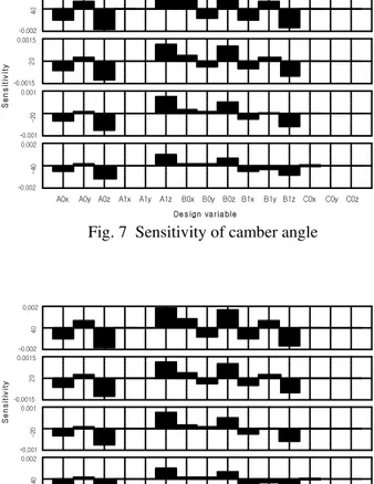
A. Sensitivity Analysis

(5)

A0x A0y A0z A1x A1y A1z B0x B0y B0zB1x B1yB1z C0x C0y C0z

40

-4

0

-2

0

20

0.002

-0.002 0.0015

-0.0015 0.001

-0.001 0.002

-0.002

De s ign va r ia ble

S

e

n

s

it

iv

it

y

Fig. 7 Sensitivity of camber angle

A0x A0y A0z A1x A1y A1z B0x B0y B0zB1x B1yB1z C0x C0y C0z

40

-4

0

-2

0

20

0.002

-0.002 0.0015

-0.0015 0.001

-0.001 0.002

-0.002

S

e

n

s

it

iv

it

y

Fig. 8 Sensitivity of toe angle

1

-1

A0x A0y A0z A1x A1y A1z B0x B0y B0z B1x B1y B1z C0x C0y C0z

40

-4

0

-2

0

20

1

-1

1.5

-1.5 2

-2

S

e

n

s

it

iv

it

y

Fig. 9 Sensitivity of kingpin inclination angle

0.5

-0.5

A0x A0yA0z A1x A1y A1z B0x B0y B0zB1x B1y B1z C0x C0y C0z

40

-4

0

-2

0

20

0.5

-0.5

0.5

-0.5 0.5

-0.5

S

e

n

s

it

iv

it

y

Fig. 10 Sensitivity of caster angle

Also, Table 7 shows the summary of the sensitivity results where the most dominant design variables to wheel alignment and forces/moments most sensitive to the design variables are specified.

Table 7 Summary of sensitivity results

Wheel alignment

The most dominant design variables to wheel alignment

Forces and moments most sensitive to the design

variables

A0z fc0x

A1z fc0x, fj1y, fc0y

B0z fb0x, fa0x

Toe

B1z fb0x, fa0x

C0y fc0x, fa0x, fj1y, fa0y

Camber

C0z fc0x, fa0x, fc1y, fa0y

A1y fb0x, fa0x

C0y fc0x, fa0x, fj1y, fa0y

K.P.I.

C0z fc0x, fa0x, fc1y, fa0y

A1x fb0x, fa0x, fa0y, MA0z

Caster

C0x fa0x, fa0y, fb0x, MA0z

B. Performance Index

For optimal design of suspension systems, the performance index (I) is selected as follows:

I = ∫[f(z)-R(z)]2dz (13)

where f is a static design factor obtained in Section 4 and R is its target value, and z is wheel travel.

The multi-performance index can be written as combination of each performance index with weights as

caster KPI

toe

camber . I . I . I

I .

I=10 +20 +20 +10 (14)

Here, relatively higher weights for toe and kingpin inclination angles are imposed since deviations between f and R are greater than others through wheel travel.

C. Optimization

The optimal design problem is formulated as:

)

x

(

I

min

n

i

x

t

s

.

_i_l

≤

_i

≤

_iu

,

=

1 ,

…

,

(15)

(6)

Table 8 Comparison of hard point between designs

X(mm) Y(mm) Z(mm)

Initial Optimum Initial Optimum Initial Optimum

A -3.00 -4.64 400.00 398.23 -125.00 -126.94

A1 2.00 -1.28 699.00 697.14 -150.00 -152.36

B0 151.00 149.12 295.00 294.01 30.00 _9.052

B1 137.00 134.89 637.00 634.86 13.00 12.01

C0 42.00 40.37 550.00 549.12 510.00 508.11

D1 0.00 -0.79 597.00 595.26 -50.00 -52.13

G 322.00 321.04 380.00 378.92 -114.00 -116.85

P1 0.00 732.50 -50.00

Fig. 11 Optimum design result of camber angle

Fig. 12 Optimum design result of toe angle

Fig. 12. Optimum design result of toe angle

Fig. 13 Optimum design result of kingpin angle

Fig. 14 Optimum design result of caster angle

VI. CONCLUSION

Optimal design of McPherson strut suspension system has been studied. Also, sensitivity analyses for the kinematic static design factor and for reaction forces at joints are carried out, from which the effects of each hard point(design variable) on suspension factors can be found. These studies may be applicable effectively to determine suspension system layout by predicting the variations of suspension factors required for vehicle characteristics at early design stages. The method employed can be extended to develop the integrated suspension design system.

.

REFERENCES

[1] Gillespie, T.D., “Fundamentals of Vehicle Dynamics, SAE, U.S.A., 1992, pp.237-274.

[2] Suh, C. H., “Synthesis and Analysis of Suspension Mechanisms with Use of Displacement Matrices”, SAE paper 890098, 1989.

[3] Suh, C. H., “Suspension Analysis with Instant Screw Axis Theory”, SAE paper 910017, 1991.

[4] Suh, C. H. and Smith, C. G., “Dynamic Simulation of Suspension Mechanisms Using the Displacement Matrix Method”, SAE paper 962222, 1996.

[5] Kang, H. Y. and Suh, C. H., “Synthesis and Analysis of Spherical- Cylindrical (SC) Link in the McPherson Strut Suspension Mechanism”, ASME J. of Mechanical Design, Vol. 116, 1994, pp.599-606. [6] Lee, J. M. , “Implementation of Analyses of Instantaneous Screw Axis

and Sensitivity of Multi-link Suspension System”, M.S. Thesis, Korea University, 1996.

[7] Tak, T. O., “Dynamic Optimum Design of Suspension System Using Sensitivity Analysis, KSAE paper, Vol.2, No.3, 1994, pp.50-60. [8] Min, H. K. and Tak T. O. and Lee, J. M., “Kinematic Design Sensitivity

Analysis of Suspension Systems Using Direct Differentiation”, KSAE paper Vol. 5, No. 1, 1997, pp.38-48.

[9] Suh, C. H., “Computer-Aided Design of Mechanisms”, Banghan Publishing Co., Seoul, 1984.