Abstract—This paper presents the importance of formulating general discrete-time model representations for current pathway deterministic modeling study. Discrete-time models can be considered as a link between continuous-time kinetic reactions and discrete-time experimentation as well as computer based simulation and analysis. In the paper, different discretization techniques are investigated according to different sorts of ODE model structures. Two discretization strategies are mainly focused, that are one-step Taylor/Lie series based method and multi-step Runge-Kutta method. A new discretization approach based on Taylor expansion and Carleman linearization is proposed for bilinear in states pathway models. Finally, the superiority of using Runge-Kutta based approach as general discrete-time model representations are concluded.
Index Terms—Biochemical pathway modeling, discretization, sensitivity analysis, systems biology.
I. INTRODUCTION
Based on large amounts of experiments, traditional biochemists and molecular biologists have developed many qualitative models and hypothesis for biochemical pathway study [1]-[3]. However, in order to evaluate the completeness and usefulness of a hypothesis, produce predictions for further testing, and better understand the interaction and dynamic of pathway components, qualitative models are no longer adequate. There has recently been a focus on more quantitative approach in systems biology study. In the past decade, numerous approaches for quantitative modeling of biochemical dynamics are proposed, such as Robert [4], Anand and Douglas [5], Jeff et al. [6], Robert and Tom [7], Tyson et al. [8], Wolkenhauer [9] [10], etc. Among these approaches, the most prominent method is to use ordinary differential equations (ODEs) to model biochemical reactions according to mass action laws. It should be noted that using ODEs to model biochemical reactions assumes that the system is well-stirred in
Manuscript received May 21, 2007. This work is supported by Hong Kong Research Grant Council, Grant No. 9041041 and partially supported by City University of Hong Kong, CityU Grant No. 7001821, and No. 122305.
F. He is with The University of Manchester, UK, and City University of Hong Kong, Hong Kong (phone: +852-2784-4154; fax: +852-2788-7791; e-mail: [email protected]).
L. F. Yeung is with Electronic Engineering Department, City University of Hong Kong, Hong Kong (e-mail: [email protected]).
M. Brown is with the School of Electronic and Electrical Engineering, The University of Manchester, Manchester M60 1QD, United Kingdom. (e-mail: [email protected]).
a homogeneous medium and that spatial effects, such as diffusion, are irrelevant, otherwise partial differential equations (PDEs) should be used [11]. In the literature, almost all publications related to pathway modeling are based on continuous-time ODE model representations. Using continuous-time ODEs facilitate researchers on analytical study and understanding, whereas it also brings difficulties for numerical computation and computer based simulation. Therefore, constructing the corresponding discrete-time model representations is particular important in systems biology study.
There are many reasons to formulate discrete-time model representations in pathway modeling research. Firstly the real biochemical kinetic reactions take place in continuous time, whereas experimental data are measured by sampling the continuous biochemical reaction outputs, and computer based analysis and simulation all depend on discrete-time datasets. Therefore, a discrete-time model could be an interface between real kinetic reaction, experimentation and computer based simulation. A delicate discrete-time model can not only assist people to better understand pathway reaction dynamics and reproduce the experimental data, but also generate predictions for computer based analysis which leaves out the expensive and time consuming experiment process. Moreover, it can be a crucial tool for further experimental design study, such as state measurement selection and sampling time design. Secondly, as we know parameter estimation is an active and important research topic in systems biology study. Estimating parameters of continuous ODEs is usually a computational costly procedure, as even for linear ODEs it is a non-quadratic optimization problem. Whereas when considering discrete-time based models, although we can not change the fundamental nature of the optimization process, however, an iterative polynomial discrete-time model could possibly simplify the structure of continuous ODEs, especially for some nonlinear cases. This can help researchers to develop new parameter estimation approaches based on the discrete-time models. Furthermore, dynamic sensitivity analysis plays an important role in parameter selection and uncertainty analysis for system identification procedure [12], in practice, local sensitivity coefficients are obtained by solving the continuous sensitivity functions and model ODEs simultaneously. As sensitivity functions are also a set of ODEs with respect to sensitivity coefficients, it would be worthwhile to calculate sensitivity coefficients in a similar discrete-time iterative way.
In practice, there are several methods can be considered for discretization of ODEs. One sort of methods is based on Taylor
Discrete-Time Model Representation for
Biochemical Pathway Systems
Fei He, Member IAENG, Lam Fat Yeung and Martin Brown
or Lie series expansion which is one-step-ahead discretization stratagem. For models represented by linear ODEs which means linear in states, the discrete-time model representation is given in discrete-time control system textbooks [13] as linear ODEs can be expressed as state-space equations. Unfortunately, for nonlinear ODEs there is no such general direct discretization mapping. In mathematical and control theory, some discretization techniques related to nonlinear ODEs are comparatively reviewed and discussed in section 3. Considering real biological signaling cases, we investigate a time varying linear approach for bilinear in states ODEs situation based on Taylor expansion and Carleman linearization. However, even for this method the mathematical model expression would be complex when considering higher order approximation. Another important discretization strategy discussed in this paper is multi-step discretization approach based on Runge-Kutta method. One advantage of this approach is it improves the discretization accuracy by utilizing multi-step information for approximation of one-step-ahead model prediction. Moreover, it gives a general exact discrete-time representation for both linear and nonlinear biochemical ODE models.
II. CONTINUOUS-TIME PATHWAY MODELING A. Continuous-Time Model Representation
In the literature [14] [15], signal pathway dynamics can usually be modeled by the following ODE representation:
( ) ( ( ), ( ), ), ( )0 0 ( ) ( ( ))
t t t t x
t t
= =
=
x f x u θ x
y g x (1)
where x∈ m
, u∈ p
, and θ∈ n
are the state, input and parameter column vectors. x0 is the initial states vector at t0. From biochemical modeling viewpoint, x represents molecular concentrations; u generally represents external cellular signals; θ stands for reaction rates. f( )⋅ is a set of linear or nonlinear functions which correspond to a series of biochemical reactions describing pathway dynamics. g( )⋅ here is the measurement function which determines which states can be measured. For the simplest case, if all the states can be measured, the measurement function g in (1) is an identity matrix. Otherwise,
g is a rectangular zero-one matrix with corresponding rows with respect to unmeasurable states deleted from the full rank identity matrix Im.
When model ODEs are linear and time invariant in states, which is also known as linear ODEs, (1) can be simplified as:
( ) ( ) ( )
( ) ( ( ))
t t t
t t
= +
=
x Ax Bu
y g x (2)
Here Am m× is the parameter matrix, Bm p× is the known input matrix. For most systems biology pathway models A is typical a sparse matrix, only the corresponding reaction state terms appear in the forcing function. However, this kind of linear ODEs is not prevalent for representation of most biochemical reactions, only if it is an irreversible chain reaction. An illustrative example is the first-order isothermal liquid-phase chain reaction [16] [17]:
1 2
A→ →θ B θ C
It states from liquid reaction component A to liquid product B and then to liquid product C. This reaction process can be model by following ODEs:
1 1 1 2 1 1 2 2
x x
x x x
θ
θ θ
= −
= − (3)
where x x1, 2 denote concentrations of components A and B, which were the only two concentrations measured. Therefore, component C does appear in the model. This ODE model (3) can be readily represented as linear state space form (2). More generally, and more applicably, we can consider ODEs that are linear in their unknown parameters, but not necessarily states. For instance, the Michaelis-Menten enzyme kinetics [20] [21], JAK-STAT [18], ERK [19], TNFα−NF−κB [20] and
I Bκ −NF−κB [15] pathway models are all bilinear in the states but linear in parameters. The state function of this kind of ODEs can be represented as:
x( )t =F x( ( ))t θ (4) where F( )⋅ represents a set of nonlinear functions which is also commonly presence as a sparse matrix. For example, considering a bilinear in states model, when a reaction only takes place in the presence of two molecules, most elements of the corresponding row in F would be zeros except for those related to this two states. Here we do not take account of model inputs u(t) as most of these published pathways are not considered subject to external cellular signals.
B. Parameter Estimation
Given the model structure and experiment data of measured state variables, the aim of parameter estimation is to calculate the parameter values that minimize some loss function between the model’s prediction and measurement data. Considering the set of { ( )}y ki i k, as the measurement data and the corresponding model’s predictions { ( , )}y ki θ i k, , which is simply discrete-time sampling of continuous-time ODE model’s output y(t), then a standard least squares loss function along the trajectory gives:
2
1
ˆ arg min ( ( ) ( , ))
2 i kωi y ki y ki
=
∑ ∑
−θ θ (5)
where the double sum can be taken simply as taking the expected value over all states (i) and over the complete trajectory (k), ωi are the weights to normalize the contributions of different state signals and can be taken as
(
)
21 max( ( ))
i i k y k
ω = (6) We assume that the model hypothesis space includes the optimal model, so that when θ θˆ= *, the model’s parameter are correct and y ki( , )θˆ =y k*i( ). Typically, we assume that the states are not directly measurable, but are subject to additive measurement noise:
y ki( )=y k*i( )+ℵ(0,σi2) (7) Here, the noise is zero mean Gaussian, where the variances depend on the state.
of states to time (left-hand-side of ODEs), so even for linear ODE models, the optimization problem is not quadratic. In the literature, parameter estimation of pathway ODEs is usually reduced into solving nonlinear boundary value problem using multiple shooting method [22]-[24].
C. Sensitivity Analysis
Dynamic sensitivity analysis plays an important role in parameter selection and uncertainty analysis for system identification procedure. The first-order local sensitivity coefficient
s
i j, is defined as the partial derivative of ith state to jth parameter,
( , ) ( , )
( )
( ) i i j j i j
i j
j j
x t x t
x t
s t θ θ θ
θ θ
+ ∆ −
∂
= =
∂ ∆ (8)
In (8), sensitivity coefficient is calculated using finite difference method (FDM), however, the numerical values obtained may vary with ∆θj, and repeated measurement of
state is required at least once for each parameter. In practice [15], direct differential method (DDM) is employed as an alternative by taking partial derivative of (1) with respect to parameter θj, and the absolute parameter sensitivity equations can be written as:
0 0
, ( )
j j j j j j j
d
S J S P S t S
dt θ x θ θ
∂ ∂ ∂ ∂
= + ⇔ = ⋅ + =
∂ ∂ ∂ ∂
x f x f
(9) where J and Pj are the Jacobian matrix and parameter
Jacobian matrix. By solving the m equations in (1) and n m× equations in (9) together as a set of differentical equations, both
( )t
x and ( )S t m n× can be determined simultaneously.
For ODEs are linear in both parameters and states, a special case described in (2), and when assuming biochemical reactions are autonomous which means do not affected by external inputs u, the corresponding linearized sensitivity equations can be expressed as:
S( )t =AS( )t +P( )t (10) where P is the m n× parameter Jacobian matrix.
For linear in the parameters ODEs (4), the corresponding sensitivity equations can be simplified as:
( ( ( ) )
( )t =∂ t ( )t + ( ( ))t
∂
F x θ
S S F x
x (11)
Parameter sensitivity coefficients provide crucial information for parameter importance measurement and further parameter selection. A measure of the estimated parameters’ quality is given by the Fisher information matrix (FIM):
2 2
T
T
d d
d d
σ σ
= =
x x
F S S
θ θ (12)
which is a lower bound on the parameter variance/covariance matrix. This is a key measure of identifiability which determines how easily the parameter values can be reliably estimated from the data, or alternatively, how many experiments would need to be performed in order to estimate the parameters to a pre-defined level of confidence.
In the literature, several algorithms for parameter selection are proposed based on parameter sensitivity analysis [26] [27]. Besides, many optimal experimental design methods [27]-[29]
are developed based on maximize the information of FIM according to commonly used optimal design criteria [30].
III. DISCRETE-TIME MODEL REPRESENTATION Equation (1)describes pathway dynamics in continues time. However, in real experiment the measurement results are obtained by sampling continues time series, and later on system analysis, parameter estimation and experimental design are all based on these discrete data sets. Therefore, it’s important to formulate a discrete time model representation.
A. One-Step System Discretization
For linear in the states ODEs, the exact discrete-time representation of system ODEs (2) will take the form:
(k+ = ⋅1) ( )k + ⋅ ( )k
x G x H u (13) If we denote t=kTand λ = −T t, where,
(
0)
, T
T
e e dλ λ
= A =
∫
AG H B (14) If matrix A is nonsingular, then H given in (14) can be simplified to
(
)
1 10 ( ) ( )
T
T T
e dλ λ − e e −
=
∫
A = A − = A −H B A I B I A B (15)
Similarly, if the biochemical reactions are autonomous, the discrete-time sensitivity equations can be written as:
(k+ = ⋅1) ( )k + d ( )k
S G S B P (16) where,
0
T d e d
λ λ
=
∫
AB (17) The discrete-time representation discussed above had been mentioned in some pathway modeling literature [31] [32].
Unfortunately, there is no general exact mapping between continuous and discrete time systems when ODEs are nonlinear. In numerical analysis and control theory, there are several methods had been discussed for one-step discretization of nonlinear ODEs. Such as finite differences method [33], which comprises Euler’s method and finite order Taylor series approximation, Carleman linearization [34], Jacobian linearization [35], feedback linearization [35], Monaco and Normand-Cyrot’s method [36] [37], etc. However, as mentioned previously not all biochemical pathway systems are subject to external cellar signals, therefore Jacobian and feedback linearization approaches which aim at design a complex input signal would not be discussed in this paper. In this section, we propose a time-varying linear approach based on Taylor expansion and Carleman linearization method for discretization of bilinear in the states pathway ODEs, and also briefly investigate Monaco and Normand-Cyrot’s scheme.
1) Taylor-Carleman Method
We initially consider a generally nonlinear model of the form:
( )t = ( ( ),t )
x f x θ (18) Then using Taylor expansion around the current time instant t=tk, the state value at the next sample point t=tk+T is given by:
1
( )
( ) ( )
!
k
l l
k k l
l t t
T t
t T t
l t
∞
= =
∂
+ = +
∂
∑
xx x (19)
which can be further simplified as: [ ] 1
( 1) ( ) ( )
!
l l l
T
k k k
l
∞
=
+ = +
∑
x x x (20) As discussed in Section 2, for some bioinformatics systems, the nonlinear ODEs are simply bilinear in the states:
x=Ax+Dx⊗x (21) where ⊗ denotes the Kronecker product and 2
m m× matrix D
is assumed to be symmetric in the sense that the coefficients corresponding to x1x2 and x2x1 are the same in value. For many biochemical pathway models, D is generally very sparse. So lets evaluate the first few derivative terms of (20) to deduce the overall structure of the exact discrete time model of (21):
2
2
( 2 ( ))( ) 2 ( )( )
= + ⊗
= + ⊗
= + + ⊗ ⊗ + ⊗ ⊗ ⊗
x Ax Dx x
x Ax Dx x
A x AD D A I x x D D I x x x
2
3 2 2
2( 2 ( ))( ) 6 ( )( )
( 2 ( ) 4 ( ) )( )
(2 ( ) 4 ( )( )
= + + ⊗ ⊗ + ⊗ ⊗ ⊗
= + + ⊗ + ⊗ ⊗ +
⊗ + ⊗ ⊗ +
x A x AD D A I x x D D I x x x
A x A D AD A I D A I x x
AD D I D A I D I
6 ( )( ))( )
6 ( )( )( )
⊗ ⊗ ⊗ ⊗ ⊗ +
⊗ ⊗ ⊗ ⊗ ⊗ ⊗
D D I A I I x x x
D D I D I I x x x x (22)
It can be seen that it is a polynomial in x of degree m+1. Hence the infinite sum in (19) is an infinite polynomial. We can notice that the coefficient of x in nth order derivative expansion is An, and the coefficient of the second order terms x⊗x can be expressed recursively:
1
1 2 1( )
n n n
q
q − q −
=
= + ⊗
D
A D A I
(23) The exact representation of (21) in discrete time should have the form:
(k+ =1) ( ( ))k
x p x (24) where requires p to be a vector valued. Here, instead of treating the system as a global non-linear discrete time representation, it would be possible to treat it as a time-varying linear system, where the time varying components depend on x. It’s obviously an infinite degree polynomial and some finite length approximation must be used instead. For instance, if we only consider the second order approximation of derivative terms in (22) and using jth order Taylor expansion, the discrete-time representation of (21) can be expressed as:
[ ] 1
1
( 1) ( ) ( )
!
( ) ( ( ) ( ) ( ))
!
l j
l l
l j
l l l
T
k k k
l T
k k q k k
l =
=
+ = +
= + + ⊗
∑
∑
x x x
x A x x x
(25)
The advantage of this approach is it gives a finite polynomial discrete time representation for bilinear in states models. However, as shown in (22) the model expression would be complex when considering exact higher order derivative expansion, otherwise, the lower order approximation of derivatives have to be employed as in (25), and corresponding discretization accuracy would decrease accordingly.
2) Monaco and Normand-Cyrot’s Method
In stead of approximating derivatives, a recent algebraic discretization method proposed by Monaco and Normand -Cyrot is based on Lie expansion of continuous ODEs. When considering nonlinear ODEs with the form (18), the corresponding discretization scheme can be expressed as:
1
( 1) ( ) ( ( ))
!
l j
l l
T
k k k
l =
+ = +
∑
fx x L x (26)
where the Lie derivative is given by
1
( ( ))
m i i i
k f
x =
∂ =
∂
∑
fx x
L (27)
and the higher order derivatives can be calculated recursively 1
( ( )) ( ( ( )))
l l
k = − k
f x f f x
L L L (28) Thus, (26) can be rewritten as:
2 3
1 1
( 1) ( ) ( ) ( ( ) )
2 6
k+ = k +T + T J ∗ + T J J ∗ ∗ +
x x f f f f f f …
(29) where J( )⋅ is the Jacobian matrix of the argument. This truncated Taylor-Lie expansion approach has been shown with accurate discrete-time approximation and superior robust performance especially when considering large sampling time step in discretization [37] [38]. However, this approach could also be computational expansive as a series of composite Jacobian matrices need to be calculated.
B. Multi-Step System Discretization
Runge-Kutta methods [25] which are widely used for solving ODEs’ initial value problems can be a nature choice for discrete time system representation. Runge-Kutta methods propagate a solution over an interval by combining the information from several Euler-style steps (e.g. (30)), and then using the information obtained to match a Taylor series expansion to some higher order.
(k+ =1) ( )k +h ( ( ))k
x x f x (30)
Here, h is the sampling interval, tk+1= +tk h.
The discrete time representation of continues-time pathway model (1) can be written as follows using Runge-Kutta method:
( 1) ( ) ( ( )) ( 1) ( ( 1))
k k k
k k
+ = +
+ = +
x x R x
y g x (31)
Here, R x( ( ))k represents the Runge-Kutta formula. According to desired modeling accuracy, different order Runge-Kutta formula can be employed, and corresponding
( ( ))k
R x would be different. For instance, the second-order Runge-Kutta formula with the expression:
1
2 1
2 ( ( ))
( ( ) 2) ( ( ))
d h k
d h k d
k d
=
= +
=
f x
f x
R x
(32)
where ( )f ⋅ is the right-hand side of model’s ODEs in (1). The most often used classical fourth-order Runge-Kutta formula is:
1
2 1
3 2
4 3
1 2 3 4
( ( ))
( ( ) 2)
( ( ) 2)
( ( ) )
( ( )) 6 3 3 6
d h k
d h k d
d h k d
d h k d
k d d d d
= = + = + = + = + + + f x f x f x f x R x (33)
In practice, fourth-order Runge-Kutta is generally superior to second -order due to four evaluations of the right-hand side per step h.
Compared with one-step discretization approaches discussed in previous subsection, the main advantage of using Runge-Kutta method for discretization is it utilizes multi-step information for approximation of one-step-ahead predictions. This strategy enhances the discretization accuracy and reduces the complexity of the mathematical expressions compared with using higher order derivative approximation in one-step discretization. Moreover, Runge-Kutta method could provide a general discrete-time ODE representation for either linear or nonlinear ODEs, whereas for one-step strategy using Taylor expansion it’s difficult to formulate a close representation for nonlinear ODEs, instead some finite order approximation has to be used.
Similarly, now the parameter sensitivity equations (9) can also be discretized using Runge-Kutta method:
(k+ =1) ( )k + S( ( ))k
S S R S (34) Here within the Runge-Kutta formula R SS( ( ))k , fS( )⋅
represents the right-hand side of sensitivity equations (9), e.g.
( ( )) ( ( ))
S k =J t k +P
f S S (35) Thus, parameter sensitivity coefficients (8) and Fisher information matrix (12) can now be represented and calculated iteratively using discrete-time formula (34).
In this section, two sorts with three kinds of discrete-time model representation methods are investigated for pathway ODEs in depth. The Runge-Kutta based method shows superiority in mathematical model expression especially for discretization of nonlinear ODEs. In next section, the simulation results of five discrete-time models based on these three approaches are discussed and compared numerically and graphically using Michaelis-Menten kinetic model.
IV. SIMULATION RESULTS
In this section, a simple pathway example is employed for illustration of different discussed discretization approaches. The accuracy and computational cost of different methods are compared as well. The example discussed here is the well known Michaelis-Menten enzyme kinetics. The kinetic reaction of this signal transduction pathway can be represented as:
3 1
2
S E ES E P
θ θ
θ
+ → + (36) Here, E is the concentration of an enzyme that combines with a substrate S to form an enzyme substrate complex ES. The complex ES holds two possible outcomes in the next step. It can be dissociated into E and S, or it can further proceed to form a product P. Here, θ1, θ2 and θ2 are the corresponding reaction
rate. The pathway kinetics described in (36) can usually be represented by the following set of ODEs:
1 1 1 2 2 3 2 1 1 2 2 3 3 3 1 1 2 2 3 3 4 3 3
( )
( )
x x x x
x x x x
x x x x
x x
θ θ
θ θ θ
θ θ θ
θ = − + = − + + = − + = (37)
Here four states x1, x2, x3 and x4 refer to S, E, ES and P in (36) respectively. As it is a set of linear in the parameter and bilinear in state ODEs, (37) can be written into matrix form:
= + ⊗
x Ax Dx x (38) Firstly, we consider one-step-ahead discretization methods discussed in Section 3. For the Taylor series and Carleman linearization based method, according to (20), the first and second order local Taylor series approximation can be expressed as:
(k+ =1) ( )k +T k( )
x x x (39) 2
(k+ =1) ( )k +T k( )+T 2 ( )k
x x x x (40)
As shown in (22), here
( ) ( ) ( ) ( )
( ) ( ) 2 ( ) ( )
k k k k
k k k k
= + ⊗
= + ⊗
x Ax Dx x
x Ax Dx x (41)
In this example,
2 1 2 3 2 2 3 3 3 4
0 0 0
0 0 0
,
0 0 ( ) 0
0 0 0
x x x x θ θ θ θ θ θ + = = − + x A 1 1 1
0 0 0 0 0 0 0 0 0 0 0 0 0 0 0
0 0 0 0 0 0 0 0 0 0 0 0 0 0 0
0 0 0 0 0 0 0 0 0 0 0 0 0 0 0
0 0 0 0 0 0 0 0 0 0 0 0 0 0 0 0
θ θ θ − − = D (42) We can notice that, for this simple kinetic example with only four state variables, matrix D ( 2
m m× ) is already in large scale. For Monaco and Normand-Cyrot’s method, here we employ a truncated third order Lie expansion for simulation. As shown in (29), we only need to notice f represnets the right hand side expression of model ODE
1 1 2 2 3 1 1 2 2 3 3 1 1 2 2 3 3 3 3
( )
( )
( )
x x x
x x x
x x x
x
θ θ
θ θ θ
θ θ θ
θ − + − + + = − +
f x (43)
The general Lie series expansion (29) seems concise in expression, however, the composite Jacobian expression would be large in scale and computational costly.
Now we consider the multi-step discretization approach based on Runge-Kutta method. It is straightforward to formulate the second and fourth order Runge-Kutta discrete-time expression using (31)-(33). For this example, we just need to replace f( )⋅ with (43), and as all the states can be measured for this example, the measurement function g is an identity matrix I4, therefore:
(k+ =1) (k+1)
Comparing the discrete-time model expression using local Taylor-Carleman expansion, Monaco and Mormand-Cyrot’s method, and Runge-Kutta method, the expression using Runge-Kutta method is more straightforward and compact, we only need to replace f x( ) with the right-hand side expression of the specific biochemical reaction ODEs. On the contrary, the discrete representation using second-order Taylor expansion is already a bit complicated as the scale of D matrix would become very large as the parameter dimension increases. As discussed in Section Ⅲ. A, it would be even more difficult to formulate a model expression using third or higher order Taylor expansion.
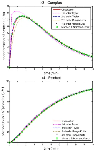
The time series simulation using different discrete-time model expressions are displayed and compared in Fig. 1. Here, five discrete-time models, which are based on first and second order Taylor expansion, second and fourth order Runge-Kutta, and Monaco and Mormand-Cyrot’s respectively, are employed for comparison. The initial values of states are: x1(0)=12,
2(0) 12
x = , x3(0)=0, x4(0)=0. Parameter values are set to be: θ1=0.18, θ2 =0.02, θ1 =0.23. Simulation time period is from 0 to 10 with sampling interval 0.3. We solve the model’s ODEs (37) using ode45 function in Matlab with sampling interval 0.1, and suppose the result as an approximation of real system observation and to be a judgment of different discretization methods. The residual mean squared errors (RMSE) between different models’ outputs and the observation are listed and compared in Table I.
0 1 2 3 4 5 6 7 8 9 10 0
2 4 6 8 10 12
time(min)
c
oncent
rat
ion of
pr
ot
ei
ns
(
µ
M)
x1 - Substrate
Observation 1st order Taylor 2nd order Taylor 2nd order Runge-Kutta 4th order Runge-Kutta Monaco & Normand-Cyrot
0 1 2 3 4 5 6 7 8 9 10 3
4 5 6 7 8 9 10 11 12
time(min)
c
oncent
rat
ion of
pr
ot
ei
ns
(
µ
M)
x2 - Enzyme
Observation 1st order Taylor 2nd order Taylor 2nd order Runge-Kutta 4th order Runge-Kutta Monaco & Normand-Cyrot
0 1 2 3 4 5 6 7 8 9 10 0
1 2 3 4 5 6 7 8 9
time(min)
c
oncent
rat
ion of
pr
ot
ei
ns
(µ
M)
x3 - Complex
Observation 1st order Taylor 2nd order Taylor 2nd order Runge-Kutta 4th order Runge-Kutta Monaco & Normand-Cyrot
0 1 2 3 4 5 6 7 8 9 10 0
2 4 6 8 10 12
time(min)
c
oncent
rat
ion of
pr
ot
ei
ns
(µ
M)
x4 - Product
Observation 1st order Taylor 2nd order Taylor 2nd order Runge-Kutta 4th order Runge-Kutta Monaco & Normand-Cyrot
Fig. 1 Time series simulation results of using five different discrete-time models
TABLE I
Time Series Simulation Residual MSE of Different Models RMSE
1st order Taylor
2ndorder Taylor
2nd order Runge-Kutta
4th order Runge-Kutta
Monaco & Normand-Cyrot x1 0.4771 0.0205 0.0942 0.0306e-4 0.0020 x2 0.5054 0.0144 0.1019 0.0774e-4 0.0030 x3 0.5054 0.0144 0.1019 0.0774e-4 0.0030 x4 0.0503 0.0105 0.0020 0.1770e-4 0.0002 Total 1.5381 0.0598 0.3000 3.6249e-5 0.0083
Fig. 1 and Table I provide states’ trajectory simulation results based on five different discrete-time models. It is clearly to see that the discrete-time model based on first-order Taylor series gives the worst approximation results with the largest RMSE, and the one based on fourth-order Runge-Kutta gives the closest simulation result to the real observation with the smallest RMSE. Besides, the discrete-time model using Monaco and Normand-Cyrot’s method and second order Taylor series also give an acceptable approximation results with relatively small RMSEs to the real observation.
V. CONCLUSION
kinetic reactions and discrete-time experimentation. It will receive more and more attentions as computer based simulation and analyses are widely used in current biochemical pathway modeling study. Two important sorts of discretization methods are mainly investigated in this paper. One strategy is based on one-step-ahead Taylor or Lie series expansion. This kind of method could give an exact discrete-time representation for linear ODEs, however, for more typical bilinear or nonlinear ODEs pathway models, truncated finite order Taylor/Lie series approximation have to be used. The mathematical discrete-time expression using higher order Taylor/Lie expansion can be very complex and it would be computational costly as well. The alternative is the Runge-Kutta based approaches, which are multi-step discretization strategy. The mathematical model representation using this method is straightforward and compact, and the simulation approximation result using fourth-order Runge-Kutta is superior to others as well. Synthetically speaking, Runge-Kutta based discretization method can be a better choice for discrete-time model representation in pathway modeling study, and the corresponding discrete-time model structure will be a useful and promising tool in the future systems biology research. Further work can focus on dynamic analysis of discrete-time models and comparison with corresponding continuous model, here dynamic analysis should include model zero dynamics, equilibrium property, chaotic behavior when varying sampling step, etc. Additionally, discrete-time local and global parametric sensitivity analysis methods would also be a significant further focus for pathway modeling study.
REFERENCES
[1] M. Peleg, I. Yeh, R. B. Altman, “Modeling biological processes using workflow and Petri net models,” Bioinformatics, 18(6), pp. 825–837, 2002.
[2] A. Regev, W. Silverman, E. Shapiro, “Representation and simulation of biochemical processes using π -calculus process algebra,” Pacific Symposium on Biocomputing 2001, pp. 459–470.
[3] S. Eker, M. Knapp, K. Laderoute, P. Lincoln, J. Meseguer, K. Sonmez, “Pathway logic: symbolic analysis of biological signaling,” Pacific Symposium on Biocomputing 2002, pp. 400–412.
[4] D. P. Robert, “Development of kinetic models in the nonlinear world of molecular cell biology,” Metabolism, vol. 46, pp. 1489-1495, 1997. [5] R. A. Anand, A.L. Douglas, “Bioengineering models of cell signaling,”
Annu. Rev. Biomed. Eng. 2000, vol.2, pp. 31-53.
[6] H. Jeff, M. David, I. Farren, J.C. James, “Computational studies of gene regulatory networks: In numero molecular biology,” Nat. Rev. Genet, vol. 2, pp. 268-279, 2001.
[7] D. P. Robert, M. Tom, “Kinetic modeling approaches to in vivo imaging,” Nat. Rev. Mol. Cell Biol, vol. 2, pp. 898-907, 2001.
[8] J. J. Tyson, C. Kathy, N. Bela, “Network dynamics and cell physiology,” Nat. Rev. Mol. Cell Biol, vol. 2, pp. 908-916, 2001.
[9] O. Wolkenhauer, “Systems Biology: The reincarnation of systems theory applied in biology?” Henri Stewart Publications, vol. 2, No. 3, pp. 258-270, 2001.
[10] K.-H. Cho, O. Wolkenhauer. “Analysis and modeling of signal transduction pathways in systems biology,” Biochemical Society Transactions, vol. 31, Part 6, pp. 1503-1509, 2003.
[11] D. B. Kell, J. D. Knowles, “The role of modeling in systems biology,” in Systems modelling in cellular biology: from concept to nuts and bolts, eds. Z. Szallasi, J. Stelling and V. Periwal, MIT Press, Cambridge, 2006. [12] M. S. Eldred, A. A Giunta, B. G. Van Bloemen Waanders, S. F.
Wojtkiewicz JR, W. E. William, M. Alleva, “DAKOTA, A Multilevel Parallel Object-Oriented Framework for Design Optimization, Parameter
Estimation, Uncertainty Quantification, and Sensitivity Analysis Version 3.0,” Technical Report, Sandia National Labs., US, 2002.
[13] O. Katsuhiko, Discrete-time Control System, U.S.A, Prentice-Hall, 2nd ed, 1995, pp. 312–515
[14] E. D. Sontag, “Molecular systems biology and control,” European J. of Control, vol. 11, pp. 1-40, 2005.
[15] H. Yue, M. Brown, D. Kell, J. Knowles, H. Wang and D. Broomhead, “Insights into the behaviour of systems biology models from dynamic sensitivity and identifiability analysis: a case study of an NF-kB signalling pathway,” Mol. BioSyst., vol. 2(12), pp. 640-649, 2006. [16] I. B. Tjoa, L. T. Biegler, “Simultaneous solution and optimization
strategies for parameter estimation of differential-algebraic equation systems,” Industrial and Engineering Chemistry Research, vol. 30, pp. 376-385, 1991.
[17] W. R. Esposito, C. A. Floudas, “Deterministic global optimization in isothermal reactor network synthesis,” Journal of Global Optimization, vol. 22, pp. 59-95, 2002.
[18] J. Timmer, T. G. Muller, I. Swameye, O. Sandra, U. Klingmuller, “Modeling the nonlinear dynamics of cellular signal transduction”, International Journal of Bifurcation and Chaos, vol. 14, No. 6, pp. 2069-2079, 2004.
[19] K-H. Cho, S-Y. Shin, H-W. Kim, O. Wolkenhauer, B. McFerran, W. Kolch. “Mathematical Modeling of the Influence of RKIP on the ERK Signaling Pathway,” Computational Methods in Systems Biology (CMSB’03). vol. 2602 of Lecture Notes in Computer Science, Springer-Verlag, 2003.
[20] K-H. Cho, S-Y. Shin, H-W. Lee, and O.Wolkenhauer, “Investigations in the Analysis and Modelling of the TNFalpha Mediated NF-kappaB Signaling Pathway,” Genome Research, vol. 13, pp. 2413-2422, 2003. [21] A.E.C. Ihekwaba, D. S. Broomhead, R. L. Grimley, N. Benson and D. B.
Kell. “Sensitivity analysis of parameters controlling oscillatory signalling in the NF-kB pathway: the roles of IKK and IkBa,” IET Systems Biology, vol 1, No.1, pp.93-103, 2004.
[22] B. van Domselaar and P. W. Hemker, “Nonlinear parameter estimation in initial value problems,” Technical Report NW 18/75, Mathematical Centre, Amsterdam, 1975.
[23] T. G. Mueller, N. Noykova, M. Gyllenberg, J. Timmer, “Parameter identification in dynamical models of anaerobic wastewater treatment,” Mathematical Biosciences, vol. 177-178, pp. 147-160, 2002.
[24] M. Peifer, and J. Timmer, “Parameter estimation in ordinary differential equations for biochemical processes using the method of multiple shooting”, IET Systems Biology, vol 1, Issue 2, pp. 78-88, 2007. [25] W. H. Press, S. A. Teukolsky, W. T. Vetterling, B. P. Flannery, Numerical
Recipes in C: the art of scientific computing, Cambridge: University Press, 1992, 2nd ed, ch. 16.
[26] R. Li, M. A. Henson and M. J. Kurtz, “Selection of model parameters for off-line parameter estimation,” IEEE Trans. on Control systems technology, vol. 12, No. 3, pp. 402-412, 2004.
[27] K. Z. Yao, B. M. Shaw, B. Kou, K. B. McAuley, and D. W. Bacon, “Modeling ethylene/butene copolymerization with multi-site catalysts: parameter estimability and experimental design,” Polym. React. Eng., vol. 11, pp. 563–588, 2003.
[28] D. Faller, U. Klingmuller, J. Timmer, “Simulation methods for optimal experimental design in systems biology,” Simulation, vol. 79, Issue 12, pp. 717-725, 2003.
[29] Z. Kutalik, K-H. Cho, and O. Wolkenhauer, “Optimal sampling time selection for parameter estimation in dynamic pathway modeling,” Biosystems, vol. 75(1-3), pp. 43-55, July 2004.
[30] A. C. Atkinson, Optimum Experimental Designs, New York: Oxford University Press, 1992.
[31] K. G. Gadkar, R. Gunawan, F. J. Doyle, “Iterative approach to model identification of biological networks,” BMC Bioinformatics, vol. 6, pp. 155, 2005.
[32] K. G. Gadkar, J. Varner, F. J. Doyle, “Model identification of signal transduction networks from data using a state regulator problem,” IEE Systems Biology, vol. 2, Issue 17, 2005
[33] C. R. Wylie, L. C. Barrett, Advanced Engineering Mathematics, 6th ed, New York: McGraw-Hill, 1995.
[34] K. Kowalski, W-H. Steeb, Nonlinear Dynamical Systems and Carleman Linearization, Singapore: World Scientif, 1991.
[35] A. Isidori, Nonlinear Control Systems, 3rd ed, London: Springer, 1995. [36] S. Monaco, D. Normand-Cyrot, “On the sampling of a linear control
system,” Proc. IEEE 24th Conf. Dec. and Control, pp. 1457-1482, 1985.
[37] S. Monaco, D. Normand-Cyrot, “A combinatorial approach to the nonlinear sampling problem”, Lecture Notes in Control and Information Sciences, vol. 114, eds. M. Thomas and A. Wymer (Berlin: Springer) pp. 788-797, 1990.
[38] E. Mendes, C. Letellier, “Displacement in the parameter space versus spurious solution of discretization with large time step”, Journal of Physics A: Mathematical and General, vol. 37, pp. 1203-1218, 2004.