On the Internal Multi-Model Control of Uncertain
Discrete-Time Systems
Chakra Othman
Laboratory L.A.R.A, NationalEngineering School of Tunis Tunis Elmanar University
Tunis, Tunisia
Ikbel Ben Cheikh
Laboratory L.A.R.A, NationalEngineering School of Tunis Tunis Elmanar University
Tunis, Tunisia
Dhaou Soudani
Laboratory, L.A.R.A, NationalEngineering School of Tunis Tunis Elmanar University
Tunis, Tunisia
Abstract—In this paper, new approaches of internal
multi-model control are proposed to be applied for the case of the discrete-time systems with parametric uncertainty. In this sense, two implantation structures of the internal multi-model control are adopted; the first is based on the principle of switching and the second on the residues techniques. The stability’s study of these control structures is based on the Kharitonov theorem, thus two extensions of this theorem have been applied to define the internal models. To illustrate these approaches, simulation results are presented at the end of this article.
Keywords—Internal model control IMC; Internal multi-model control IMMC; Kharitonov theorem; Switching method; Residues techniques; discrete-time systems; uncertain systems
I. INTRODUCTION
The robustness problem in the case of parametric uncertainties aroused great interest among researchers. Robustness means the preservation of system characteristics such as stability or performance in the presence of unknown disturbances and noise.
Different control methods to solve this problem have been proposed. The internal model control has always been considered as an efficient approach in control systems, due to its high accuracy and robustness against internal and external disturbances. This method is generally used because of its robustness; it includes an inspired internal model of the process and a controller. It’s preferable that this controller is the inverse of the internal model to ensure a perfect tracking of the reference. In this article, the internal multi-model control approach for the case of discrete-time uncertain systems is proposed to be applied.
Our contribution consists in implanting a control structure based on a multi-model controller in the discrete area by adopting two synthesis techniques namely switching technology and residues technique in order to minimize errors due to the modeling imperfections. These two techniques will be developed in this paper.
This structure contains instead of one internal model a set of models representing the process in different operating points by using multi-model approach and by consequent, a set of controllers that based on two specific inversion methods.
The system under consideration in this paper is a class of complex systems which is the discrete-time uncertain system with parametric uncertainty.
The multi-model approach is used to obtain the internal models inspired from the process of this control structure. It’s a mathematical approach designed to represent the best possible the dynamic operation of a complex process, using linear time-invariant models. The multi-model approach allows representing complex systems in the form of interpolation between linear models. Each local model is a dynamic linear time invariant system valid around an operating point. [1]
Kharitonov method is used with these two theorems [15] for the discrete-time uncertain systems to determine the internal models of the multi-model control structure.
In these control structures, synthesis of the controller is reduced to a problem of internal models inverse construction. In addition, the direct inversion of the models is often impossible. Thus, the proposed controller synthesis approach is based on a specific inversion method. This approach has been modified to improve the accuracy of the controlled system. [3,4]
II. DISCRETE-TIME UNCERTAIN SYSTEMS
In practice there are many uncertainties that affect the physical system and therefore its model. In general, two uncertainty classes are distinguished, the structured uncertainties that affect the physical parameters value of the process model and the unstructured uncertainties defined by an upper bound of the model difference in the frequency domain. [2,13]
This article focuses on a class of uncertain systems where uncertainty is parametric.
III. STABILITY STUDY OF THE DISCRETE-TIME UNCERTAIN
SYSTEMS USING KHARITONOV METHOD
The Kharitonov theorem is an important combination, generalizing the Routh-Hurwitz criterion. [10] The application of the Kharitonov theorem in the continuous case leads to false results for the uncertain discrete-time systems. This has required the development of this theorem in the discrete-time case. [14, 15, 16]
A. First extension of the Kharitonov method
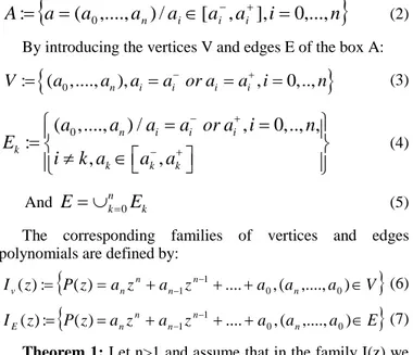
Let I(z) be the polynomials family of the following form:
0 1
1
...
)
(
z
a
z
a
z
a
P
n nn
n
+
+
+
=
−− (1)
{
a
a
a
a
a
a
i
n
}
A
:
=
=
(
0,....,
n)
/
i∈
[
i−,
i+],
=
0
,...,
(2) By introducing the vertices V and edges E of the box A:{
0}
:
(
,....,
n),
i i i i,
0,..,
V
=
a
a
a
=
a or a
−=
a i
+=
n
(3)0
( ,....,
) /
,
0,.., ,
:
,
,
n i i i
k
k k k
a
a
a
a or a i
n
E
i
k a
a a
− +
− +
=
=
=
≠
∈
(4)
And
E
= ∪
nk=0E
k (5) The corresponding families of vertices and edges polynomials are defined by:{
P z a z a z a a a V}
z
I n n
n n n
v = = + + + ∈
−
− .... ,( ,...., )
) ( : )
( 1 0 0
1 (6)
{
P z a z a z a a a E}
z
I n
n n n n
E = = + + + ∈
−
− .... ,( ,...., )
) ( : )
( 0 0
1
1 (7)
Theorem 1: Let n>1 and assume that in the family I(z) we
have fixed upper order coefficients such that ai-=ai+ for i=n/2+1, ...., n if n is even and i=(n+1)/2,....,n if n is odd. Then the entire family I(z) is stable if and only if the family of vertex polynomials Iv(z) is stable.
B. Second extension of the Kharitonov theorem
In the above theorem, the upper order coefficients are fixed, now let us consider that all the coefficients are allowed to vary, so let ‘nu’ be defined as follow:
1,
2,....,
2
2
n
n
nu
=
+
+
n
if n is even (8)(
1)
(
1)
1,
2,....,
2
2
n
n
nu
=
+
+
+
+
n
if n is odd (9)Let consider the upper edges E* which can be defined by:
0
* : ( ,...., n) / i i i, 0,.., , , k k, k , k
a a a a ou a i n i k a a a E
k nu
− + − +
= = ≠ ∈
=
∈
(10)
The upper edge polynomials are obtained by varying a single higher order parameter and fixing others at their minimum or maximum values.
The family of higher edge polynomials can be defined by:
{
}
* 1 *
1 0 0
( ) : ( ) n n .... ), ( ,..., )
E n n n
I z = P z =a z +a−z− +a a a ∈E (11) A typical upper edge in IE*(z) is defined by:
0
... (
(1
)
) ....
n k
n k k
a z
+ +
λ
a
−+ −
λ
a z
++
a
k
∈
nu
,a
i=
a
i−ora
i=
a
i+, i=0,…,n,i
≠
k
There are:
2
2
n
n
upper edges if n is even1
2
2
n
n
+
upper edges if n is oddTheorem 2: The family of polynomials I(z) is stable if and
only if the family of edge polynomials IE*(z) is stable.
IV. INTERNAL MODEL CONTROL STRUCTURE
This internal model control strategy acquired interest due to its robustness. The main advantage of this structure is the simplicity of its construction, and the easy interpretation of the roles of its blocks.[3,8]
The internal model control structure includes an internal model ‘M’ which is an explicit model of the process to be controlled and a regulator ‘C’ which can be chosen the inverse of the model and if necessary a robustness filter ‘F’ as indicated in figure (1). ‘R’, ‘d’, ‘Y’, are respectively the reference to reach, the modeling error and the system output. ‘P’ is a disturbance added at the output of the process
The internal model control structure used as a control signal the difference between the output of the process and its internal model.
In the basic structure of the IMC, the command signal “U” outcome from the corrector ‘C’ is applied simultaneously to the process ‘G’ and its model ‘M’. The IMC exploits the behavior gap to correct the error on the reference. The error signal includes the influence of external disturbances and modeling errors.
Generally the internal model control structure includes a robustness filter usually introduced in the feedback loop. Its role is to introduce certain robustness against the modeling errors.
Fig. 1. Basic structure of the internal model control structure
In this article, the presence of the filter is not taken into account.
In this control structure, the controller is chosen equal to the model inverse to ensure the equality between the process output and the reference despite the added disturbance at the output. [3]
In addition, the direct inversion of the model is often impossible, especially when the model is with no-minimum phase or presents a delay, thus, inversion methods are used. The implementation method of the approximated inverse is used for systems with a transfer function whose order of the numerator is less than the order of the denominator, non-minimum phase systems and delay systems.
Fig. 2. Basic idea to obtain the approximated inverse
The global transfer function of the scheme (2) is:
1
1
( )
1
( )
A
C z
A M z
=
+
(12)For sufficiently high values of the gain A1, the controller C(z) approaches the inverse of internal model M(z):
1
( )
( )
C z
M z
≈
(13)Thus, the global transfer function C(z) is the approximated inverse of the model transfer function M(z).
For some classes of systems, the gain A1 that ensures stability of the loop that realize the controller C(z), may not be very high, which does not allow us to obtain the approximated inverse, therefore, a gain A2 is added to ensure a null static error. Thus, a second structure of the corrector is proposed: [5, 6, 8]
Fig. 3. Structure of the second corrector used
The gain A2 is used to ensure the desired accuracy, it is described by the following expression:
1 2
1
1
(1)
(1)
A M
A
A M
+
=
(14)V. INTERNAL MULTI-MODEL CONTROL APPROACH OF
UNCERTAIN DISCRETE-TIME SYSTEMS
In order to reduce the complexity of dynamic process, the tendency has been to use linear time invariants models (LTI).
The multi-model represents complex system as an interpolation between in general linear or affine local models. Each local model is a dynamic system LTI (Linear Time Invariant) valid around an operating point.[1]
Uncertain systems can be represented by a library of linear models. These linear models are at the origin of the elaboration of a new control structure called internal multi-model control structure denoted IMMC. By combining the internal model control structure and the multi-model approach, the internal multi-model control approach is obtained.
The internal multi-model control structure for uncertain discrete-time systems was developed from the structure
described in the latest paragraph. It uses instead of a single internal model a library of models after the application of the Kharitonov’s theorem for this class of discrete-time uncertain systems.[12]
This IMMC structure exploits the difference between the output of the process and the library of models outputs.
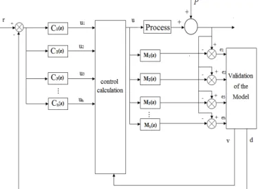
Let’s consider the following diagram of the internal multi-model control structure: [6, 8, 10, 11]
Fig. 4. Internal multi-model control structure of uncertain discrete-time systems
In this structure, the process is the uncertain discrete-time system to be controlled, M1(z), M2(z), M3(z), … , Mh(z) for i=1,..,h, represent the transfer functions of the internal models and C1(z), C2(z), C3(z), … , Ch(z) for i=1,..,h, are the transfer functions of the controllers.
In this control structure Mi(z) for i = 1, ... , h, are the linear models library inspired from the uncertain process, ‘d’ is the modeling error and ‘v’ is the validation index of the nearest model.
The proposed regulators for this control structure are the Mi-1 inverse models library that represents the inverse of the internal models Mi for i=1,..,h.
Several fusion methods were employed in the literature.
The choice of the control signal to be applied in this article is based firstly, on the switching method and secondly on the fusion method known as the residues techniques.
A. First IMMC structure based on the switching principle This first method consists of determining the closest model to the process that allows to have the least modeling error. The control signal to be applied is therefore the signal that corresponds to the model that leads to the slightest error.
Fig. 5. Diagram of the first internal multi-model control structure of uncertain discrete-time systems based on switching method
In the basic diagram of this structure A1, A2, A3, … , Ah are the gains used for the inverse models.
Among the different Kharitonov models, the model that has the slightest error is chosen. The selected controller is then obtained from the model, whose output is nearest to the process, the validation block ensures the choice of this model.
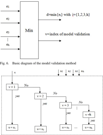
The figures (6) and (7) represent the block diagram of the model validation method and the diagram describing the principle of control calculation.
Fig. 6. Basic diagram of the model validation method
Fig. 7. Basic diagram for computing the control signal
For some classes of systems, the gain Ai with i∈[1, .. ,h] that ensures stability of the loop that realize the controllers
Ci(z) for i=1,..,h, may not be very high, which does not allow us to obtain the approximated inverses, therefore, a gain A2i for i=1,..,h is added to ensure a null static error. Thus, using the second structure of the proposed corrector described in figure (3), a second internal multi-model control structure which is based on the switching principle is obtained:
Fig. 8. Diagram of the second internal multi-model control structure of uncertain discrete-time systems based on switching method
B. Second IMMC structure based on the residues techniques of the uncertain discrete-time systems
The second internal multi-model control structure assumes the same internal models but the choice of the control signal to be applied is based on the principle of fusion known as residues techniques.
Using the inversion methods described previously for the realization of the inverse models, the first diagram of the internal multi-model control structure based on the residues techniques is obtained:
Fig. 9. First diagram of the internal multi-model control structure for discrete-time uncertain systems based on residues techniques
The calculation of the global command to apply to the system depends on partial control signals related to the models Mi and on the validities of these models.
Validity indexes are inversely proportional to the difference between the system output and the outputs of the internal models that can be defined by:
( )
( )
( )
i i
The validity can be expressed by the expression (16):
1
1
1
i ih
j j
d
v
d
=
=
∑
(16)
Thus, the global control signal can be defined by the expression (17):
1
( )
( ) ( )
h
i i
i
u t
v t u t
=
=
∑
(17) Using the second structure of the proposed corrector, a second internal multi-model control structure which is based on the residues technique is obtained:Fig. 10. Second diagram of the internal multi-model control structure for discrete-time uncertain systems based on residues techniques
VI. APPLICATION
In this paragraph, there are two parts. In the first part, the first extension of the Kharitonov theorem is used and in the second part, the second Kharitonov theorem extension is applied. In each part, there are two sections. In the first section the internal multi-model control structure based on the switching method is applied, however, in the second section, the second internal multi-model control structure based on residues techniques is considered.
A. Example 1: Using the first Khartonov theorem
1) Application of the multi-model control structure based on the swiching method:
Let’s consider the following transfer function:
0 1 2
5
.
0
)
(
a
z
a
z
z
z
G
+
+
−
=
(18)where:
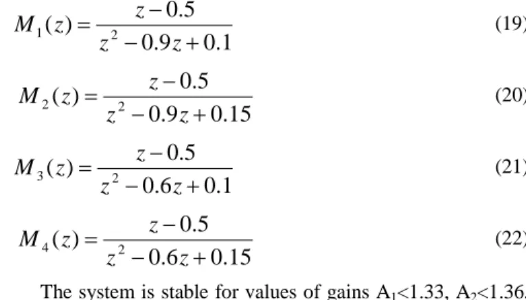
Applying the first Kharitonov theorem previously defined, the following four Kharitonov models are obtained:
1
.
0
9
.
0
5
.
0
)
(
21
−
+
−
=
z
z
z
z
M
(19)15
.
0
9
.
0
5
.
0
)
(
22
−
+
−
=
z
z
z
z
M
(20)1
.
0
6
.
0
5
.
0
)
(
23
−
+
−
=
z
z
z
z
M
(21)15
.
0
6
.
0
5
.
0
)
(
24
−
+
−
=
z
z
z
z
M
(22)The system is stable for values of gains A1<1.33, A2<1.36, A3<1.13 and A4<1.16.
During the whole application:
The sampling period is considered equal to T=0.1s
The input signal takes the form of a unit step reference
The disturbance takes the form of step with amplitude equal to 0.5 applied at k=20
The output signal by applying the first internal multi-model control structure based on the switching method for Ai=1 for i=1,…,4 is presented in the figure 11. The output signal oscillate at startup, this is due to the switching of the control signal. Also, the system presents a non-null error on the steady-state, this is because the gains Ai for i=1,..,4 that ensure stability of the loop that realize the controller C(z) are not very high, which does not allow us to obtain the approximated inverses, thus, a gains A2i for i=1,..,4 are added to ensure a null static error. It is therefore preferable to apply the second internal multi-model control structure based on the switching technique.
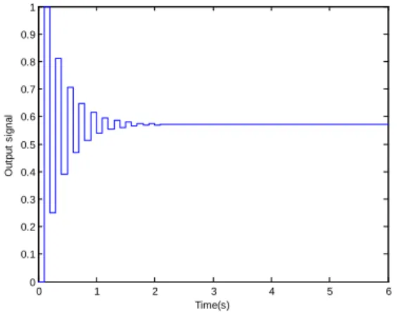
The output signal for Ai=1 for i=1,…,4 and A21=1.4, A22=1.5, A23=2, A24=2.11 is displayed in the figure 12. The output of this uncertain process presents oscillation in transient regime and quickly reaches the reference in steady state.
By adding a disturbance at the output, the output signal for the same gains values Ai and A2i for i=1,..,4 is displayed in the figure 13. This control structure has rejected the external disturbance.
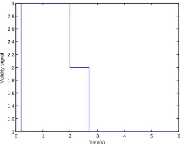
The figure 14 displays the validity signal, this signal lets us show the chosen model and therefore the selected controller applied.
For a sampling period T=1s and for the same gains values Ai and A2i, the figure 15 shows the output signal. The system takes longer time to stabilize that with a period ten times smaller.
[
]
0
0.1, 0.15
a
∈
[
]
1
0.9, 0.6
Fig. 11. Output signal for Ai=1 for i = 1,..,4 and for a sampling period T=0.1s
Fig. 12. Output signal for Ai=1 for i=1,..,4 and A21=1.4, A22=1.5, A23=2, A24=2.11 and for a sampling period T=0.1s
Fig. 13. Output signal by adding a disturbance for Ai=1 for i=1,..,4 and A21=1.4, A22=1.5, A23=2, A24=2.11 and for a sampling period T=0.1s
Fig. 14. Validity signal for Ai=1 for i=1,..,4 and A21=1.4, A22=1.5, A23=2, A24=2.11 and for a sampling period T=0.1s
Fig. 15. Output signal for a sampling period T=1s, for Ai=1 for i=1,..,4 and for A21=1.4, A22=1.5, A23=2, A24=2.11
2) Application of the multi-model control structure based on the residues techniques:
The same example previously studied in the last paragraph and defined by the transfer function (18) and the four internal models (19, 20, 21, 22) is considered in this paragraph.
The output signal by applying the first internal multi-model control structure based on residues techniques for Ai=1 for i=1,…,4 is presented in the figure 16. As previously, this first control structure with internal multi-model based on residues techniques does not allow us to obtain perfect results, the system output presents static errors. It is preferable to apply the second internal multi-model control structure based on residues techniques.
By applying the second internal multi-model control structure based on residues techniques, the output signal for Ai=1 for i=1,…,4 and A21=1.4, A22=1.5, A23=2, A24=2.11 is displayed in the figure 17. It’s noted that the transient state presents oscillation then the process output converges well to the reference.
0 1 2 3 4 5 6
0 0.1 0.2 0.3 0.4 0.5 0.6 0.7 0.8 0.9 1
Time (s)
O
ut
put
S
ignal
0 1 2 3 4 5 6
0 0.5 1 1.5
Time (s)
O
ut
put
S
ignal
0 1 2 3 4 5 6
0 0.5 1 1.5
Time(s)
O
ut
put
s
ignal
0 1 2 3 4 5 6 1
1.2 1.4 1.6 1.8 2 2.2 2.4 2.6 2.8 3
Time(s)
V
al
idi
ty
s
ignal
0 5 10 15
0 0.5 1 1.5
Time(s)
O
ut
put
s
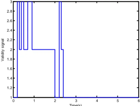
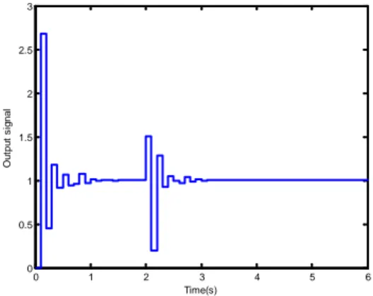
By adding a disturbance at the output, the output signal for the same gains values is presented in the figure 18. This second internal multi-model control structure allows to reject the external disturbance. The figure 19 displayed the validity signals of the different models. These signals are used for the computing of the control signal.
For a period T=1s, the output signal for the same gains values is displayed in the figure 20. By increasing the value of the sampling period T, the system takes more time to stabilise.
Fig. 16. Output signal for Ai=1 for i=1,...,4
Fig. 17. Output signal for Ai=1 for i=1,..,4 and A21=1.4, A22=1.5, A23=2, A24=2.11 and for a sampling period T=0.1s
Fig. 18. Output signal by adding a disturbance for Ai=1 for i=1,..,4 and A21=1.4, A22=1.5, A23=2, A24=2.11 and for a sampling period T=0.1s
Fig. 19. Validities signals for Ai=1 for i=1,..,4 and A21=1.4, A22=1.5, A23=2, A24=2.11 and for a sampling period T=0.1s
Fig. 20. Output signal for a sampling period T=1s, Ai=1 for i=1,..,4 and for A21=1.4, A22=1.5, A23=2, A24=2.11
Satisfactory results have been obtained with this two internal multi-model control structure. The amplitude of the oscillations in the transient state for the case of the second structure based on the fusion method is somewhat higher compared to the first structure based on the switching method. However, by using this second structure, the system has reached the reference and has rejected the disturbance more rapidly.
B. Example 2: Using the second Kharitonov theorem
1) Application of the multi-model control structure based on the switching method:
Let’s consider the transfer function of the uncertain system defined by the expression (23):
2
2 1 0
(
0.5)
( )
z
G z
a z
a z
a
−
=
+
+
(23)where:
0 1 2 3 4 5 6 0
0.1 0.2 0.3 0.4 0.5 0.6 0.7 0.8 0.9 1
Time(s)
O
ut
put
s
ignal
0 1 2 3 4 5 6 0
0.2 0.4 0.6 0.8 1 1.2 1.4 1.6 1.8
Time(s)
O
ut
put
s
ignal
0 1 2 3 4 5 6 0
0.2 0.4 0.6 0.8 1 1.2 1.4 1.6 1.8
Time(s)
O
ut
put
s
ignal
0 1 2 3 4 5 6 0
0.1 0.2 0.3 0.4 0.5 0.6 0.7 0.8 0.9 1
Time(s)
V
al
idi
ty
s
ignal
s
v1 v2 v3 v4
0 2 4 6 8 10 12 0
0.2 0.4 0.6 0.8 1 1.2 1.4 1.6 1.8
Time(s)
O
ut
put
s
ignal
[
]
0
0.2, 0.8
a
∈
[
]
1
0.1, 0.25
a
∈ −
[
]
2
2.5, 4
It is clear that the system can be written in the poly-topical form, therefore by applying the second theorem, the following twelve edges polynomials can be determined by varying one parameter and setting the others.
)
6
.
0
8
.
0
(
1
.
0
5
.
2
)
,
(
21
λ
z
=
z
−
z
+
−
λ
E
(24))
6
.
0
8
.
0
(
25
.
0
5
.
2
)
,
(
22
λ
z
=
z
+
z
+
−
λ
E
(25))
6
.
0
8
.
0
(
1
.
0
4
)
,
(
23
λ
z
=
z
−
z
+
−
λ
E
(26))
6
.
0
8
.
0
(
25
.
0
4
)
,
(
24
λ
z
=
z
+
z
+
−
λ
E
(27)2
.
0
)
35
.
0
25
.
0
(
5
.
2
)
,
(
25
z
=
z
+
−
z
+
E
λ
λ
(28)8
.
0
)
35
.
0
25
.
0
(
5
.
2
)
,
(
26
z
=
z
+
−
z
+
E
λ
λ
(29)2
.
0
)
35
.
0
25
.
0
(
4
)
,
(
27
z
=
z
+
−
z
+
E
λ
λ
(30)8
.
0
)
035
25
.
0
(
4
)
,
(
28
z
=
z
+
−
z
+
E
λ
λ
(31)2
.
0
1
.
0
)
5
.
1
4
(
)
,
(
29
z
=
−
z
−
z
+
E
λ
λ
(32)8
.
0
1
.
0
)
5
.
1
4
(
)
,
(
210
z
=
−
z
−
z
+
E
λ
λ
(33)2
.
0
25
.
0
)
5
.
1
4
(
)
,
(
211
z
=
−
z
+
z
+
E
λ
λ
(34)8
.
0
25
.
0
)
5
.
1
4
(
)
,
(
212
z
=
−
z
+
z
+
E
λ
λ
(35) According to the second theorem defined above, the stability of the uncertain system can be checked by studying the four higher models. This system is stable if and only if these four higher polynomials are stable.By studying these four models, we find that the uncertain system is stable thereafter, the four higher Kharitonov models for λ=0.5 are proposed to be considered as the four internal models of the multi-model control structure.
2
.
0
1
.
0
25
.
3
5
.
0
)
(
21
−
+
−
=
z
z
z
z
M
(36)8
.
0
1
.
0
25
.
3
5
.
0
)
(
22
−
+
−
=
z
z
z
z
M
(37)2
.
0
25
.
0
25
.
3
5
.
0
)
(
23
+
+
−
=
z
z
z
z
M
(38)8
.
0
25
.
0
25
.
3
5
.
0
)
(
24
+
+
−
=
z
z
z
z
M
(39)The process is stable for gains A1<2.36, A2<2.76, A3<2.13, A4<2.86.
The output signal by applying the first internal multi-model control structure based on the switching method for Ai=1, for i=1,…,4 is displayed in the figure 21. The static error is different to zero in the steady state that’s because the gains Ai for i=1,…,4 that ensure stability of the loop that realize the controller C(z) are not very high. Thus the second internal multi-model control structure based on the switching method is proposed to be applied.
By applying the second internal multi-model control structure based on the switching method, the output signal for Ai=1 for i=1,…,4 and A21=7.9, A22=8.9, A23=8.4, A24=9.6 is shown in the figure 22.
The figure 23 represents the validity signal for the same gains values Ai and A2i for i=1,..,4. This figure shows the switching between the models and consequently between the control signals in the transient state. After, one second the validity signal has stabilized and the second controller has commanded the system.
By adding a disturbance at the output, the output signal is shown in the figure 24. The use of this control structure allowed us to reject the external disturbance.
The addition of external disturbance leads to more switching between models. This is shown in the figure 25 that displayed the validity signal for this case.
For a sampling period T=1s, the output signal for the same gains values Ai and A2i for i=1,..,4 is displayed in the figure 26. From this figure, it’s clear that for the same value of the gains Ai and A2i for i=1,..,4, the system takes more times to stabilize.
Fig. 21. Output signal for Ai=1, for i=1,…,4 and T=0.1s
0 1 2 3 4 5 6
(b) : Output signal
Fig. 22. Output signal for Ai=1, for i=1,…,4 and A21=7.9, A22=8.9, A23=8.4, A24=9.6 and for a sampling period T=0.1s
Fig. 23. Validity signal for Ai=1, for i=1,…,4 and A21=7.9, A22=8.9, A23=8.4, A24=9.6 and for a sampling period T=0.1s
Fig. 24. Output signal by adding external disturbance for Ai=1, for i=1,…,4 and A21=7.9, A22=8.9, A23=8.4, A24=9.6 and for T=0.1s
Fig. 25. Validity signal for the case of the disturbance presence and for Ai=1, for i=1,…,4 and A21=7.9, A22=8.9, A23=8.4, A24=9.6 and for T=0.1s
Fig. 26. Output signal for a sampling period T=1s and for Ai=1, for i=1,…,4 and A21=7.9, A22=8.9, A23=8.4, A24=9.6
2) Application of the multi-model control structure based on the residues techniques:
Let’s consider the same example previously studied in the preceding paragraph where the transfer function of the system is defined by (23) and the four internal models are given by (36, 37, 38 and 39).
The output signal by applying the first internal multi-model control structure based on fusion method for Ai=1 for i=1,..,4 is presented in the figure 27. The system output does not follow properly the reference and it present low oscillations in transient state. Thus, it’s better to apply the second internal multi-model control structure based on the residues techniques.
By applying the second internal multi-model control structure based on the residues techniques, the output signal for Ai=1, A21=7.9, A22=8.9, A23=8.4 and A24=9.6 for i=1,...,4 is shown in the figure 28. Satisfactory results have been obtained by the application of this second internal multi-model control structure based on residues techniques, it has enabled us to have null static errors.
By adding disturbance at the output, the figure 29 displays the output signal. This second internal multi-model control
0 1 2 3 4 5 6
0 0.5 1 1.5 2 2.5
Time(s)
O
ut
put
s
ignal
0 1 2 3 4 5 6
1 1.2 1.4 1.6 1.8 2 2.2 2.4 2.6 2.8 3
Time(s)
V
al
idi
ty
s
ignal
0 1 2 3 4 5 6
0 0.5 1 1.5 2 2.5
Time(s)
O
ut
put
s
ignal
0 1 2 3 4 5 6 1
1.2 1.4 1.6 1.8 2 2.2 2.4 2.6 2.8 3
Time(s)
V
al
idi
ty
s
ignal
0 2 4 6 8 10 12 0
0.5 1 1.5 2 2.5
Time(s)
O
ut
put
s
structure based on residues techniques leads to reject the added disturbance.
The figure 30 displays the validity signals of the different models. This figure shows the validity of the different internal models used for the calculation of the control signal.
For a sampling period T=1s, the output signal for the same gains values Ai and A2i for i=1,..,4 are presented in figures 31. From this figure, it’s clear that the system takes longer time to reach the reference.
Fig. 27. Output signal for Ai=1, for i=1,…,4 and for a sampling period T=0.1s
Fig. 28. Output signal for Ai=1, for i=1,…,4 and A21=7.9, A22=8.9, A23=8.4, A24=9.6 and for a sampling period T=0.1s
Fig. 29. Output signal by adding external disturbance for Ai=1, for i=1,…,4 and A21=7.9, A22=8.9, A23=8.4, A24=9.6 and for T=0.1s
Fig. 30. Validity signals for Ai=1, for i=1,…,4 and A21=7.9, A22=8.9, A23=8.4, A24=9.6 and for T=0.1s
Fig. 31. Output signal for Ai=1, for i=1,…,4 and A21=7.9, A22=8.9, A23=8.4, A24=9.6 and for T=1s
Satisfactory results have been obtained with this two internal multi-model control structure.
The second Kharitonov method leads to best results compared to the first method. The oscillations in the transient state decreased and the output signals have reached the reference more rapidly relatively.
VII. CONCLUSION
In this article, the internal multi-model control structures IMMC have been applied for the case of the discrete-time uncertain systems. The first internal multi-model control structure is based on the approach of switching between the different models. On the other hand, the second internal multi-model control structure is based on the residues techniques.
The Kharitonov method has been used for the study of the uncertain discrete-time systems. Linear models were obtained by applying this method with their two extensions for the case of the discrete-time uncertain systems.
These two control approaches have been applied for this class of systems, the discrete-time uncertain systems which can be represented by a linear model library. These linear models
0 1 2 3 4 5 6 0
0.05 0.1 0.15 0.2 0.25 0.3 0.35
Time(s)
O
ut
put
s
ignal
0 1 2 3 4 5 6 0
0.5 1 1.5 2 2.5 3
O
ut
put
s
ignal
Time(s)
0 1 2 3 4 5 6 0
0.5 1 1.5 2 2.5 3
Time(s)
O
ut
put
s
ignal
0 1 2 3 4 5 6 0
0.1 0.2 0.3 0.4 0.5 0.6 0.7 0.8 0.9
Time(s)
V
al
idi
ty
s
ignal
s
v1 v2 v3 v4
0 2 4 6 8 10 12 0
0.5 1 1.5 2 2.5 3
Time(s)
O
ut
put
s
obtained by using the Kharitonov method are considered as internal models of these control structures.
The controller synthesis approach proposed is based on a specific inversion method. This approach has been modified to improve the accuracy of the controlled system.
These different control structures have been successfully applied for the case of uncertain discrete-time systems.
By applying the first extension of the Kharitonov method, the second internal multi-model control structure based on residues techniques led to good results in terms of speed compared to the internal multi-model control structure based on the switching method.
The second extension of the Kharitonov method leads to better results compared to the first method. The oscillations in the transient state have decreased clearly.
In this article, the robustness of the proposed internal multi-model control approaches overlooked the multi-modeling errors and the external disturbances has been shown.
The choice of the sampling frequency strongly influences on the response of the system, a high value of the sampling frequency leads to more time taken to stabilize.
However, these satisfactory results invite us to improve the structure of our control approach whatsoever at the level of our controller or at the control loop level to improve the system performance in particular rejecting the effect of uncertainty whatever the synthesis approach.
REFERENCES
[1] M. Chadli, “Stabilité et commande de systèmes décrits par des structures multimodèles,” Thèse de doctorat, Institut National Polytechnique de Lorraine, december 2002.
[2] M. Morari and E. Zafiriou, “Robust process control”, Prentice Hall, Englewood Cliffs, 1989.
[3] C.E. Garcia and M. Morari, “Internal Model Control 1- A unifying review and some results”, Ind. Eng. Chem. Process Des. Dev., vol. 21, pp. 403-411, 1982.
[4] L. Saidi, “Commande a modèle interne: Inversion et équivalence structurelle ”, Thèse de doctorat, INSA de Lyon, France,1990.
[5] M. Benrejeb, M. Naceur and D. Soudani., “On an internal model controller based on the use of a specific inverse model”, International Conference on Machine Intelligence, ACIDCA’2005, Tozeur, pp. 623-626, 2005.
[6] M. Naceur, “ Sur la commande par modèle interne des systèmes dynamiques continus et échantillonnés”, Thèse de doctorat, Ecole Nationale d’Ingénieurs de Tunis, february 2008.
[7] M. Naceur, D. Soudani, M. Benrejeb. “Sur la commande par modèle interne des systèmes échantillonnés basée sur une inversion spécifique, ”, JTEA’ 2006, Hammamet 2006.
[8] C.Othman, I. Ben Cheikh, D. Soudani, “Application of the internal model control method for the stability study of uncertain sampled systems”, CISTEM 2014 IEEE Tunis.
[9] M. Naceur, I. Ben Cheikh, D. Soudani, M. Benrejeb, “On the Internal Model Control of Uncertain Systems”, 978-1-4244-7534-6/10/$26.00 ©IEEE, Juin 2010.
[10] D. Soudani, M. Naceur, K. Ben Saad. and M. Benrejeb, “On an internal multimodel control for nonlinear systems – A comparative study”, Int. J. Modelling, Identification and Control, Vol. 5, No. 4, pp. 320-326, 2008. [11] M. Naceur, D. Soudani, M. Benrejeb, P. Borne “On internal multimodel
control for nonlinear system,” IMACS, CESA 2006, Beijing, pp 306-310,2006.
[12] Z. Sun, J. Chen, X. Zhu, “Multi-model internal model control applied in temperature reduction system”, Proceeding of the 11th World Congress on Intelligent Control and Automation Shenyang, China, June 29 - July 4, 2014.
[13] N.K.Sinha and Whou Qi-Jie, “ Discrete_time approximation of multivariable continuous_time systems”, IEE PROC., Vol 130, Pt. D, No. 3. May 1983.
[14] K. Yeung, S. Nang, “A simple proof of Kharitonov’s Theorem”, IEEE Trans. On Automatic Control, Vol. AC-32, No. 9, Sept 1987.
[15] P. P. Vaidyanathan, “A New Breakthrough In Linear-System Theory: Kharitonov’s Result”, California Institute of Technology, Pasadenia, CA 91125, 1988.