Nonlinear Pricing beyond the Demand Profile
Approach
A. Araujo
a,b, H. Moreira
band S. Vieira
aaInstituto Nacional de Matem´atica Pura e Aplicada, Estrada Dona Castorina 110,
Rio de Janeiro, Brasil
bGraduate School of Economics, Getulio Vargas Foundation, Praia de Botafogo,
190, Rio de Janeiro, Brasil
Abstract
Wilson [16] introduced a general methodology to deal with monopolistic pricing in situations where customers have private information on their tastes (‘types’). It is based on the demand profile of customers: For each nonlinear tariff by the monopolist the demand at a given level of product (or quality) is the measure of customers’ types whose marginal utility is at least the marginal tariff (‘price’). When the customers’ marginal utility has a natural ordering (i.e., the Spence and Mirrlees Condition), such demand profile is very easy to perform. In this paper we will present a particular model with one-dimensional type where the Spence and Mirrlees condition (SMC) fails and the demand profile approach results in a suboptimal solution for the monopolist. Moreover, we will suggest a generalization of the demand profile procedure that improves the monopolist’s profit when the SMC does not hold.
1 Introduction
Nonlinear pricing schemes are widely used in many markets such as mobile telephony, fixed telephony, electricity and gas supply, postal services, air and railroad transport, cable TV and internet. For this reason, it has attracted a lot of attention over the past decades from economists. One of the seminal papers in this field is by Mussa and Rosen [10], who analysed nonlinear prices for the provision of quality-differentiated goods. Other contributions were made by Goldman, Leland and Sibley [5], who studied price discrimination via quantity discounts and by Maskin and Riley [9] who observed that all these models belong to the same class of principal-agent problems.
On the other hand, the demand profile approach is an alternative formulation for the monopolistic screening problem, introduced in the literature by Brown and Sibley [2] and then thoroughly expounded in Wilson [16]1. The basis for this approach is the requirement that the marginal tariff T′(q) cuts the
customer’s demand curve once from below. When satisfied, we have that the customer’s maximization problem is quasiconcave so its demand behavior can be deduced completely from the marginal benefit of consumption. In Goldman, Leland and Sibley, a tariff satisfying this requirement is called a single-crossing tariff, a terminology that we will also use in this paper.
All these methods work fine and equivalently when the Spence and Mirrlees condition (SMC) is satisfied. The main reason is that it provides a natural ordering for the customer’s demand curves. As a consequence, the monopolist is able to induce any monotonic decision for the customers by selecting a compatible tariff.
We study a nonlinear pricing model where the monopolist has incomplete information about the slope and the intercept of the customer’s demand curve, represented by α and β. In our model these two dimensions have antagonic effects in the decision q which should increase with α and decrease with β. We further assume that these two dimensions are dependent in a way that we can reduce it into a one-dimensional screening model with parameter θ. Now a bigger θ will represent at the same time as a bigger α and β and the monopolist does not know which of the antagonic effects will dominate the other. By having only one dimension summarizing the effects of those two parameters, it ends up in a model where the SMC is not satisfied anymore.
Without the SMC the problem becomes rather complex, in part due to the absence of this natural ordering. As a consequence the decision q may be
1 In a survey on multidimensional screening, Rochet and Stole [15] make a
nonmonotonic. Besides the local incentive compatibility conditions may not be sufficient as new global conditions arise. This problem without the SMC was studied by Araujo and Moreira [1]. Although they relax the Spence and Mirrlees condition, the optimal contract proposed there is compatible with the demand profile approach, because it is implemented by a single-crossing tariff and consequently the customers face a quasiconcave problem.
Our goal is to show that in our monopolistic screening model without the SMC, the contract resulting from a single-crossing tariff, compatible with the demand profile approach may be suboptimal for the monopolist. We present another contract that provides a larger profit for the monopolist. This contract is not compatible with the demand profile approach because the tariff is not single-crossing. Moreover the optimal contract is discontinuous and induces a separation in the quality spectrum between two groups: one who buys low quality goods, and the other who buys high quality goods. The tariff should be adjusted in a way that one group does not envy the other.
The paper is organized as follows. In Section 2 we define the model we are using. Then, in Section 3 we present some results related to the incentive compatibility condition. In Section 4 we derive the monopolist’s optimization problem using an approach adapted from Goldman, Leland and Sibley, we establish the pointwise optimality conditions for the monopolist’s problem and finally we solve some examples. In Section 6 we present the conclusions. All proofs are given in the Appendix.
2 Model
We use the Principal-Agent framework to analyse the monopolistic screening problem. In this model, each customer has a quasi-linear preference:
V(q, t, θ) = v(q, θ)−t,
where t represents the monetary transfer. The parameter θ is a random vari-able with a positive and continuous density representing the customer’s type. The firm is a profit-maximizing monopolist which can produce any quality
q∈Q⊆R+ incurring in a cost C(q).Q represents the quality spectrum. The monopolist’s revenue is given by:
Π(q, t) = t−C(q).
Using the‘Revelation Principle’ 2 the monopolist’s problem can be stated as
choosing the allocation rule (q, t) : Θ→R+×R that solves:
max
{q(·),t(·)}
Z
ΘΠ(q(θ), t(θ))p(θ)dθ, (1)
subject to the individual-rationality constraints:
v(q(θ), θ)−t(θ)≥0 ∀θ∈Θ, (IR)
and theincentive compatibility constraints:
θ∈arg max θ′∈Θ{v(q(θ
′), θ)−t(θ′)}, ∀θ∈Θ. (IC)
Remark 1 The ‘Taxation Principle’3 states that any allocation (q, t)
satis-fying the IC constraints can be implemented by a nonlinear tariff T : Q =
q(Θ) →R where:
T(q(θ)) =t(θ), ∀θ∈Θ.
2.1 The Model Setup
We consider a monopolist who produces a single good and is uncertain about the slope and the intercept of the customer’s demand curves. The utility func-tion of each customer is parametrized according to:
v(q, α, β) = αq−βq 2
2,
and the individual inverse demand curve is given by:
p(q) =α−βq.
The cross derivatives ofv satisfy:vqα >0 andvqβ ≤0. These conditions imply that an incentive compatible decisionqmust increase withαand decrease with
β (see Rochet [14]). Hence the effects of these parameters on q are antagonic.
We analyse the case when the random variablesα andβ are dependent in the following manner:
α=θ,
β =bθ2,
with θ uniformly distributed on [θ, θ] = [a, a+ 1]. Now we have then only one parameter θ to cope with the effects of α and β. A bigger θ means bigger α
and β, so the decision will increase or decrease depending on which effect is dominant. This results in the following setup:
v(q, θ) = θq−bθ2q2 2,
C(q) = cq 2
2,
and we assume that a, band c are nonnegative constants.
The inverse demand function is now given by
p(q) =θ−bθ2q,
and the elasticity of demand is
ǫ(q, θ) = 1− 1
bθq.
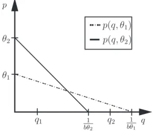
The demand function for types θ1 and θ2 are drawn in Figure 1. For θ-type customer, the ratio q = 1/(bθ) measures the market size and the intercept θ
represents the minimum price such that this customer’s demand is zero.
p
q θ1
θ2
1
bθ1
1
bθ 2
p(q, θ1)
p(q, θ2)
q1 q2
Fig. 1. Demand curves forθ1 and θ2 customers.
When b = 0 the specification of this model is the same as Mussa and Rosen [10], but whenb > 0 the Spence and Mirrlees condition4is no longer satisfied and the solution of vqθ(q, θ) = 0 determines a decreasing function given by
q0(θ) = 1
2bθ. (2)
the lack of an ordering of the demand curves as we can see in Figure 1, where we have the following inequalities for the marginal utility:vq(q1, θ1)< vq(q1, θ2) and vq(q2, θ1)> vq(q2, θ2).
Unlike the SMC case, it is not possible to know a priori which customer will consume more, as this is determined endogenously as a response to the nonlin-ear tariff adopted by the monopolist. The decision now may be nonmonotonic, increasing inCS+ and decreasing inCS− and these conditions suggest a
bell-shaped form for the decision function q.
3 Incentive Compatibility Conditions
Without the Spence and Mirrlees condition there is not a simple rule for characterizing an incentive compatible allocation and the problem becomes very complex. There are some necessary conditions, however, that should be taken into account.
In all that follows, we assume that the allocation rule (q, t) is bounded and incentive compatible. The informational rent V : Θ→R+ is given by:
V(θ) =v(q(θ), θ)−t(θ), (3)
and T :q(Θ)→R is the tariff resulting from the‘Revelation Principle’.
We begin by establishing a basic property regarding the Lipschitz continuity of bothT and V.
Lemma 1 (Differentiability Condition.) The tariff T and the informa-tional rent V are Lipschitz continuous.
Notice that Lemma 1 guarantees that both T and V are absolute continu-ous and then a.e. differentiable and now we are able to deduce the following envelope conditions involving their derivatives.
Lemma 2 (Envelope Conditions for V and T.)
(i) If V is differentiable at θ ∈int(Θ) and q ∈q(θ), then
V′(θ) = vθ(q, θ). (4)
4 The Spence and Mirrlees condition states that the cross derivative v
(ii) If T is differentiable at q∈q(θ)∩int(q(Θ)), then
T′(q) =vq(q, θ). (5)
Notice that Lemma 2 (ii) can be understood as the first order condition of the θ-customer maximization problem:
max
q∈Q{v(q, θ)−T(q)}.
With the SMC a decision is incentive compatible if and only if is monotonic. However, without the SMC we may have a nonmonotonic incentive compatible decision. The next result is related to the local monotonicity conditions on the decisionq.
Lemma 3 (Local Monotonicity Conditions.) Suppose thatq is continu-ous at θ0. Then:
(i) If q(θ0)> q0(θ0) then q is increasing at θ0,
(ii) If q(θ0)< q0(θ0) then q is decreasing at θ0,
where q0 is defined in equation (2).
The new possibilities for q coming from Lemma 3 motivates us to define the bell-shaped decisions.
Definition 1 (Bell-Shaped Decisions.) The decision q : Θ → R+ is
bell-shaped if there exists a continuity point θm ∈Θ such that the restrictions:
q|[θ,θm]is increasing and q|[θm,θ]is decreasing.
For a bell-shaped decision, we may have a discrete pooling situation, when types θ1 and θ2 choose the same decision q. Using Lemma 2 (ii), we can easily deduce a new necessary condition for incentive compatibility relating the marginal valuations of the pooled types.
Corollary 1 (Bell-Shaped Condition.) Suppose thatT is differentiable at
q∈q(θ1)∩q(θ2) an interior point of Q=q(Θ). Then
vq(q, θ1) =vq(q, θ2). (BS)
4 The Monopolist’s Problem
Suppose first that the alocation rule (q, t) is incentive compatible. Let us now deduce the monopolist’s maximization problem, using the same derivation as Mussa and Rosen [10]. From the definition of the informational rent V
(equation (3)) we can write the monetary transfer ast(θ) =v(q(θ), θ)−V(θ) and then substitute it in equation (1). The result is the following problem:
max
{q(·)}
Z
Θ{v(q(θ), θ)−C(q(θ))−V(θ)}dθ. (6)
Now using Lemma 2 and an integration by parts procedure, we can rewrite the problem above as5:
max
{q(·)}
Z θ
θ f(q(θ), θ)dθ, (ΠR)
where f(q, θ) is given by:
f(q, θ) =v(q(θ), θ)−C(q(θ)) + (θ−a−1)vθ(q(θ), θ).
This is called the relaxed version of the monopolist’s maximization problem, because the monotonicity constraints are not considered in this problem. The inconvenience of the derivation above is that in many situations the solution of Problem (ΠR) is far from being incentive compatible. One reason is that it does not consider the (BS) condition. We are going to derive the monopolist’s optimization problem in a way that the (BS) necessary condition given by Corollary 1 can be taken into account. We need the following definitions:
Definition 2 Consider a monotonic function q : [θ, θ] → R along with its upper contour set S(q) = {θ∈[θ, θ] :q(θ)≥q}.
If q is decreasing, we define ψs :R→[θ, θ] as:
ψs(q) =
supS(q), if S(q)6=∅,
θ, if S(q) = ∅.
If q is increasing, we define ψb :R→[θ, θ] as:
ψb(q) =
infS(q), if S(q)6=∅,
θ, if S(q) =∅.
5 We are implicitily assuming that V′(θ)≥0. For a more general case we refer to
In both cases, ψb and ψs are monotonic and they are denoted the
pseudoin-verses of q.
For a bell-shaped decision, using a procedure similar to Goldman, Leland and Sibley [5], we can reformulate the problem (ΠR). First we use the fundamental theorem of calculus to write:
Z θ
θ f(q(θ), θ)dθ =
Z θ
θ
Z q(θ)
q fq(q, θ)dqdθ.
Then, we use Fubini’s theorem, and the following problem results:
max
{ψb,ψs}
Z q
q {F(q, ψs(q))−F(q, ψb(q))}dq+
Z θ
θ f(q, θ)dθ. (7)
F is given by the following equation:
F(q, ψ) =
Z ψ
θ fq(q, θ)dθ, (8)
and besides ψb is the pseudoinverse of the increasing part of q and ψs is the inverse of the decreasing part of q. They are denoted type assignment functions, because they relate q with the type who purchases it. Notice that the integration variable on the left hand side of equation (7) isq, and now we can treat the constraint imposed by the condition (BS) condition for each q
separately.
4.1 Single-Crossing Tariff
First let us define a single-crossing tariff6:
Definition 3 (Single-Crossing Tariff.) A tariff is said to be single-crossing at q if, for any θ such that vq(q, θ) ≥ T′(q), vq(q′, θ) ≥ T′(q′) for q′ ≤ q. If
T(q) is single-crossing for all q, we term it a single-crossing tariff schedule.
If the tariff is single-crossing and continuous, then the customer’s maximiza-tion problem is quasiconcave.
Using the concept of a single-crossing tariff, we will be able to define the following optimization problem for the monopolist, when q(θ)< q(θ)7:
max
{ψb,ψs}
Z q
q {F(q, ψs(q))−F(q, ψb(q))}dq+
Z θ
θ f(q, θ)dθ, s.t. vq(q, ψb(q))−vq(q, ψs(q))≤0.
(ΠBS)
Notice that the problem ΠBS is coherent with a single-crossing tariffT. In this case, when q(θ)< q(θ) and q < q(θ), thenvq(q, ψb(q))≤vq(q, ψs(q)), because
T′(q) = v
q(q, ψb(q)) andvq(q, θ)≥T′(q).
Once we find the optimal type assignment functions ψb and ψs we can invert them and find the optimal decision q.
Now let us establish the optimality conditions for ΠBS.
Theorem 2 The solution ofΠBS is characterized by the following conditions:
(i) If the condition BS is not binding and θ < ψb(q)< ψs(q) = θ then:
fq(q, ψb(q)) = 0, (9)
(ii) If the condition BS is binding and θ < ψb(q)< ψs(q)< θ then:
fq(q, ψs(q))
vqθ(q, ψs(q))
= fq(q, ψb(q))
vqθ(q, ψb(q))
, (10)
(iii) If the condition BS is binding and θ < ψb(q)< ψs(q) =θ then:
vq(q, ψb(q)) = vq(q, θ). (11)
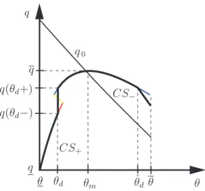
In Figure 2, we show the typical solution for the optimization problem ΠBS resulting from Theorem 2. Forq < q1, we use condition (i), forq ∈(q1, q2) we use condition (iii) and finally for q ∈(q2, q) we use condition (ii). As we can see there is a problem related with the monotonicity condition resulting from Lemma 3.
We have two alternatives for fixing this lack of monotonicity. The first one is a vertical ironing compatible with a single-crossing tariff T and the next proposition shows how restrictive this condition is.
Proposition 1 If the tariffT is single-crossing then the decision q is convex valued.
7 The other case, when q(θ) > q(θ), is treated analogously, and we only have to
q
CS+
CS− q0
θ θm
q q
θ θ
q1
q2
Fig. 2. A typical solution for ΠBS.
As a consequence of Proposition 1, if the decision q jumps at θd, then the marginal tariff for q ∈ [q(θd−), q(θd+)] is given by T′(q) = vq(q, θd) and this affects the decision for customers with typesθ close toθ. The reason is simple: with a single-crossing tariff, the marginal net benefit determines the customer’s choice and when a jump occurs, the marginal tariff is automatically defined for all the intermediate quantities and of course this may affect some customer’s decisions.
q
CS+
CS− q0
θ θm
q q
θ θd θˆd θ
q(θd+)
q(θd−)
Fig. 3. The vertical ironing procedure.
The decision function that emerges from this vertical ironing is given by:
qθd(θ) =
qR(θ) , if θ < θd,
qB(θ) , if θd≤θ ≤θˆd,
qC(θ, θd) , if ˆθd≤θ ≤θ,
whereqRandqBresult from Theorem 2 (i) and (ii), respectively. On the other hand qC results from solving the equation:
vq(q, θd) = vq(q, θ).
Notice that the customers with type θ ≥ θˆd choose q ∈ [q(θd−), q(θd+)] and their decision is affected by the fact that for this q the marginal tariff is
T′(q) = vq(q, θd). The function qC captures this effect. Finally, we get ˆθd from
solving qB(θd) =qB(ˆθd).
The point θd must be chosen optimally and is characterized by the following:
Theorem 3 The first order condition for the optimal θd is given by:
f(qB(θd), θd)−f(qR(θd), θd) =
Z θ
ˆ
θd
fq(qC(θ, θd), θ)
∂qC
∂θd
(θ, θd)dθ. (13)
Notice that this vertical ironing fixes the monotonicity problem by keeping the type assignment functionsψb andψscontinuous. This kind of solution was also proposed in Araujo and Moreira [1]. It can also be obtained by using the demand profile approach of Wilson, but the computations are more difficult than the one we presented here.
4.2 Non Single-Crossing Tariff
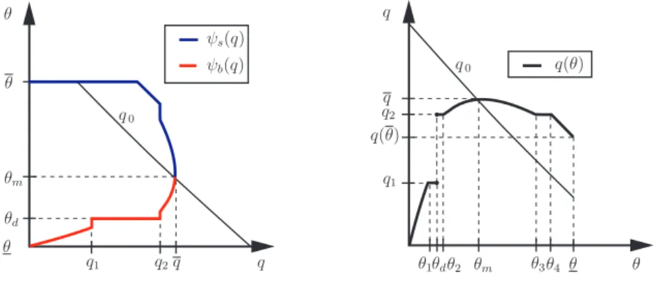
Now we propose an alternative for this vertical ironing whereψbandψsmay be discontinuous. This is illustrated in Figure 4. More than that, our procedure will result in a non single-crossing tariff.
θm
θd
θ θ
q1 q2q
θ
q θd θm θ
q2
q
q
θ1 θ2 θ3θ4
q(θ)
θ ψb(q)
ψs(q)
q(θ) q0
q0
q1
Fig. 4. An alternative ironing procedure.
We will impose the global incentive compatibility constraint relating θd and
customer. In other words we impose:
v(q(θ), θ)−t(θ)≥v(q(θd), θ)−t(θd). (14)
The following result will be useful to restate the condition above8:
Lemma 4 Consider an allocation rule (q, t) : Θ→R+×R. If (q, t)is
incen-tive compatible then:
Z θ
ˆ
θ
Z q(˜θ)
q(ˆθ) vqθ(˜q, ˜
θ)dqd˜ θ˜≥0, ∀θ,θˆ∈Θ. (15)
Notice that Lemma 4 relates incentive compatibility with an area condition represented by a double integral.
The same procedure used in the proof of Lemma 4 allows us to write the inequality (14) as:
Z θ
θd
Z q(˜θ)
q(θd)
vqθ(˜q,θ˜)dqd˜ θ˜≥0. (16)
Notice that:
Z θ
θd
Z q(˜θ)
q(θd)
vqθ(˜q,θ˜)dqd˜ θ˜=
Z θ
θd
Z q2 q1
vqθ(˜q,θ˜)dqd˜ θ˜+
Z θ
θd
Z q(˜θ)
q2
vqθ(˜q,θ˜)dqd˜ θ.˜ (17)
Using Fubini’s theorem, we can write the second integral on the right hand side of equation (17) as:
Z θ
θd
Z q(˜θ)
q2
vqθ(˜q,θ˜)dqd˜ θ˜=
Z q
q2
Z ψs(q)
ψb(q)
vqθ(˜q,θ˜)dθd˜ q˜
=
Z q
q2
{vq(q, ψs(q))−vq(q, ψb(q))}dq.
However vq(q, ψs(q)) = vq(q, ψb(q)) for q∈(q2, q] which implies that this part is null.
Using Fubini’s theorem again we can write the first integral on the right hand side of equation (17) as:
Z θ
θd
Z q2 q1
vqθ(˜q,θ˜)dqd˜ θ˜=
Z q2 q1
{vq(q, ψs(q))−vq(q, θd)}dq. (18)
8 This condition is actually equivalent to incentive compatibility, as shown by
and the condition in equation (16) will be given by:
Z q2 q1
{vq(q, ψs(q))−vq(q, θd)}dq ≥0. (ISO)
In the interval [q1, q2], we will optimally choose ψs(q) such that the condition (ISO) is fulfilled. So we have the following isoperimetric problem:
max
{ψs}
Z q2 q1
{F(q, ψs(q))−F(q, θd)}dq
s.t.(ISO).
(ΠISO)
Theorem 4 The solution of ΠISO is characterized by the following condition:
fq(q, ψs(q)) +λvqθ(q, ψs(q)) = 0, (19)
where λ is chosen to satisfy the condition (ISO) with equality.
Now we use conditions given by Theorem 2 and Theorem 4 to build a can-didate for the monopolist’s optimization problem. The cited theorems give the pointwise conditions for the three pieces that constitute the candidate we are proposing. Looking again at Figure 4, we see that the only change is for
q ∈[q1, q2], where we are doing this alternative ironing. The values q1, q2 and θd are endogenously determined as a result of an optimization process. Let us describe the type assignment functions ψb and ψs:
ψs(q) =
ψsr(q) , if q ≤q≤q1,
ψsi(q) , if q1 ≤q≤q2,
ψsc(q) , if q2 ≤q≤q,
(20)
where we have thatψsr =θ, ψsi(q) is given by equation (19) and ψsc is given by equation (10).
ψb(q) =
ψbr(q) , if q≤q≤q1,
ψbi(q) , if q1 ≤q ≤q2,
ψbc(q) , if q2 ≤q≤q,
(21)
where ψbi =θd, we define ψbr from equation (9) and ψbc from equation (10).
Now the monopolist’s problem will depend on the variablesq1, q2 and θd, and we can write its expected profit as Π(q1, q2, θd) where q1, q2 and θd satisfy the condition (ISO). Our last step is to optimally choose these parameters:
charac-terized by:
(i) F(q1, ψsr(q1))−F(q1, ψbr(q1)) +F(q1, θd)−F(q1, ψsi(q1))
vq(q1, ψsi(q1))−vq(q1, θd)
=λ,
(ii) F(q2, ψsi(q2))−F(q2, θd) +F(q2, ψbc(q2))−F(q2, ψsc(q2))
vq(q2, θd)−vq(q2, ψsi(q2))
=λ,
(iii)
Z q2 q1
{Fθ(q, θd) +λvqθ(q, θd)}dq = 0,
where λ is the Lagrangian multiplier associated with the isoperimetric con-straint.
Remark 2 Considering the isoperimetric condition, we have four equations and four parameters:q1, q2, θd and λ. We get the optimal candidate by solving
this system of equations.
5 An Example
This example illustrates the difference between the two ironing procedures used for fixing the monotonicity problem. The first one is compatible with the demand profile approach because the resulting tariff is single-crossing. The second one uses the isoperimetric condition and results in a non single-crossing tariff.
Let us choose the following values for the parameters in our model:a = 2, b= 1 and c= 6. With these parameters, we have thatθ is uniformly distributed in [2,3] and:
v(q, θ) = θq−θ2q 2
2,
C(q) = 3q2.
Using Theorem 2, we can derive the solution for ΠBS:
ψb(q) =
3q+1−√−9q2 −3q+1 3q ,if
1
6 ≤q ≤ 1 102
15 +√21,
1−3q
q , if
1 102
15 +√21≤q≤ 1 66
9 +√15, 3q−√3√q2
−24q4
6q2 , if
1 66
9 +√15≤q≤ 1 2√6.
ψs(q) =
3, if 16 ≤q ≤ 1 102
15 +√21,
3, if 1 102
15 +√21≤q≤ 1 66
9 +√15, 3q+√3√q2
−24q4
6q2 ,if 1
66
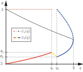
As we can see in Figure 5 ψb is nonmonotonic. We are going to derive the solutions using the two ironing procedures developed before.
ψb(q) ψs(q)
2 3
q1 q2 θ1
θ2
q q θ
Fig. 5. The solutions ψb and ψs for ΠBS.
a) Standard Ironing Procedure:
The first step is to write the solution depending on the parameter θd, as we did in equation (12):
qθd(θ) =
qR(θ) = −3θ32−2θ
+6θ−6 , if θ < θd, qB(θ) = 3θ+
√
3θ2 −12
2(3θ2+6) , if θd ≤θ ≤θˆd,
qC(θ, θd) = θ+1θd , if ˆθd ≤θ ≤θ,
where ˆθd= 2θd− √
3qθ2
d−4.
Using Theorem 3, we can find the optimal θ∗
d and ˆθ∗d:
θ∗
d ≈2.164282, ˆ
θ∗
d ≈2.89596.
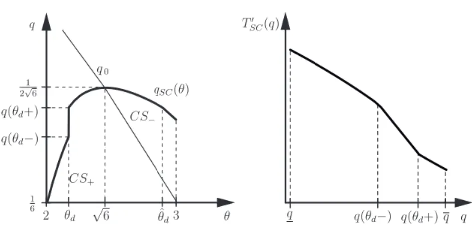
The decision fucntion resulting from this ironing procedure is denotedqSC(θ). We can find the tariff TSC(q) that implements the decision by integrating the marginal tariff given by:
TSC′ (q) =vq(q, ψb(q)),
The monopolist’s expected profit from qSC(θ) is:
Π(θd) = 0.200272 (22)
q
CS+
CS−
q0
θd θˆd
q(θd+)
q(θd−)
√
6 1
2√6
1 6
2 3 θ
T′
SC(q)
q
q q(θd−) q(θd+) q
qSC(θ)
Fig. 6. The decision function and the marginal tariff.
b) Isoperimetric Ironing Procedure:
Now we use the isoperimetric procedure. Let us describe the type assignment functions ψs and ψb according to equations (20) and (21):
ψs(q) =
ψsr(q) = 3 , if 16 ≤q≤q1,
ψsi(q) =
1−q(λ−3)+√(λ2
−6λ−9)q2+(λ −3)q+1
3q , if q1 ≤q≤q2,
ψsc(q) =
3q+√3√q2 −24q4
6q2 , if q2 ≤q≤ 1
2√6,
ψb(q) =
ψbr(q) =
3q+1−√−9q2 −3q+1 3q , if
1
6 ≤q ≤q1, ψbi(q) = θd , if q1 ≤q ≤q2,
ψbc(q) =
3q−√3√q2 −24q4
6q2 , if q2 ≤q ≤
1 2√6.
Using Theorem 5 and the isoperimetric condition, we get the following values:
q1 ≈0.183112, q2 ≈0.202431, θd≈2.201349, λ ≈0.067841.
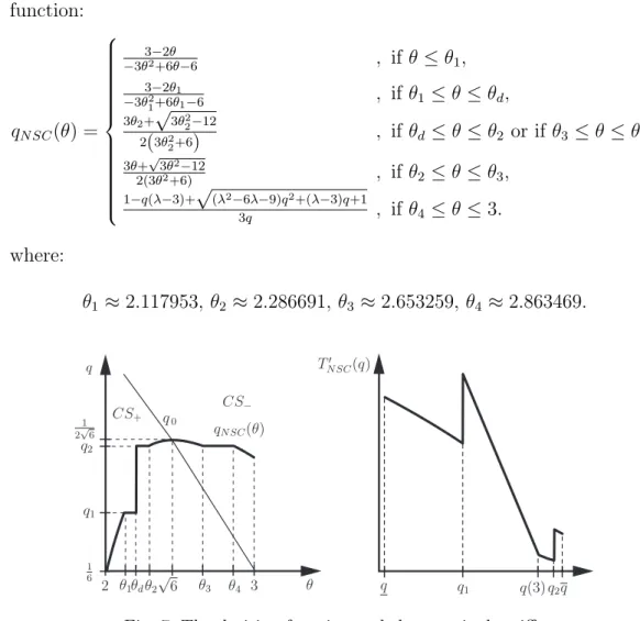
function:
qN SC(θ) =
3−2θ −3θ2
+6θ−6 , if θ ≤θ1,
3−2θ1 −3θ2
1+6θ1−6 , if θ1 ≤θ ≤θd,
3θ2+√3θ22−12
2(3θ2 2+6)
, if θd≤θ ≤θ2 or if θ3 ≤θ ≤θ4,
3θ+√3θ2 −12 2(3θ2
+6) , if θ2 ≤θ ≤θ3,
1−q(λ−3)+√(λ2
−6λ−9)q2
+(λ−3)q+1
3q , if θ4 ≤θ ≤3.
where:
θ1 ≈2.117953, θ2 ≈2.286691, θ3 ≈2.653259, θ4 ≈2.863469.
q CS+ CS− q0 θd √ 6 1 2√6
1 6
2 θ1 θ2 θ3 θ4 3 q1
q2
θ T′
N SC(q)
qN SC(θ)
q1 q(3)q2
q q
Fig. 7. The decision function and the marginal tariff..
We can find the tariff TN SC(q) that implements the decision qN SC(θ) by inte-grating the marginal tariff given by:
TN SC′ (q) =
vq(q, ψbr(q)), if 16 ≤q≤q1,
vq(q, ψsi(q)), if q1 ≤q≤q2,
vq(q, ψbc(q)), if q2 ≤q≤ 2√16.
We can see in Figure 7 the decision function qN SC(θ) and the marginal tariff
T′
N SC(q). Notice that jumps in the marginal tariff correspond to bunching in the decision function graphic.
The monopolist’s expected profit from qN SC(θ) is:
Π(q1, q2, θd) = 0.200314 (23)
increase of approximately 0.021%. This shows the suboptimality the decision function qN SC(θ).
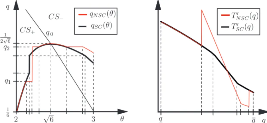
In Figure 8 we make a superposition of the decision function and the marginal tariff for ironing procedures (a) and (b). Notice that the latter results in a smaller quality spectrum than the former.
q
q q
T′
SC(q)
T′
N SC(q)
q
CS+
CS−
q0
√
6
1 2√6
1 6
2 3
q1
q2
θ qSC(θ)
qN SC(θ)
Fig. 8. The decision an the marginal tariff for both procedures (a) and (b) .
The fundamental difference between the two decision functions is that qSC(θ) is implemented by the single-crossing tariffTSC(q) andqN SC(θ) is implemented by the non single-crossing tariff TN SC(q). In fact, when the tariff is TN SC(q), the maximization problem for customer θd is not quasiconcave as it has two local maximaq1andq2so the decisionqN SC(θ) is not convex valued. In Figure 9 we plot the customer θd utility depending on his choice of q under the non single-crossing tariff TN SC(q).
q1 q2 q
V(θd)
q(θ) q(θm)
v(q, θd)−TN SC(q)
Fig. 9. The customerθd’s utility under the non single-crossing tariffTN SC(q).
6 Conclusion
not be valid and that the demand profile approach can lead to a suboptimal solution for the monopolist’s optimization problem. The reason is that the requirement of a single-crossing tariff is restrictive, as it imposes a convex valued decision.
In a multidimensional setting we also have the same situation described here, since there is not a natural ordering for the customer’s demand curves. Then one has to investigate whether the restrictions imposed by the demand profile approach may affect or not the monopolist’s welfare. Without a criterion based on the fundaments of the model that allows the monopolist to anticipate whether his maximization problem results or not in a single-crossing tariff, we cannot know if the contract resulting from the demand profile approach is a suboptimal contract. This poses a serious restriction in knowing which problems are adequate for this kind of approach.
Appendix
We need the concept of cyclical monotonicity9:
Definition 4 A correspondence q : Θ → Q is v-cyclic-monotone if and only if for all finite cycles θ0, θ1, . . . , θn+1 =θ0 ∈Θ,
n
X
i=0
{v(q(θi), θi+1)−v(q(θi), θi)} ≤0.
Theorem 6 (Rochet, 1987) A decision q : Θ → Q is implementable if and only if q is v-cyclic-monotone.
We also need some abstract convexity results related to incentive compatibility that we will state here.10
Definition 5 Let V : Θ → R. The v-subdifferential of V, ∂vV : Θ → Q, is
defined by:
∂vV(θ) =
{q∈Q:V(θ′)−V(θ)≥v(q, θ′)−v(q, θ) ∀θ′ ∈Θ}.
Definition 6 V is said to be v-subdifferentiable inΘ if and only if ∂vV(θ)
6
= ∅ ∀θ∈Θ.
Definition 7 Let V : Θ→R. We define the v-conjugated of V by:
Vv :Q→R Vv(q) = sup θ∈Θ{
v(q, θ)−V(θ)};
9 This can be found in Rochet [14].
and the v-biconjugate of V by:
Vvv : Θ→R Vvv(θ) = sup q∈Q{
v(q, θ)−Vv(q)}.
Proposition 2 Let V : Θ→R , then:
V is v-convex⇔V =Vvv.
Proposition 3 Let V : Θ→R , then:
q∈∂vV(θ)
⇔V(θ) +Vv(q) =v(q, θ).
Theorem 7 (Carlier, 2001) A decision q: Θ→RM+ is implementable if and
only if there exists a v-convex and v-subdifferentiable function V : Θ → R
such that:
q(θ)∈∂vV(θ)
∀θ ∈Ω.
Remark 1 So when the informational rent V is v-convex, the conjugate Vv
plays the role of the nonlinear tariff T that implements the decision q and the correspondence ∂vV(θ) is identified with q(θ).
Proof of Lemma 1 The v-conjugation result allows us to write:
V(θ) = max
q∈Q{v(q, θ)−T(q)}, and
T(q) = max
θ∈Θ{v(q, θ)−V(θ)}. (24)
Let us prove first thatV is Lipschitz continuous. By the incentive compatibility constraint we have that:
v(q(θ), θ)−t(θ)≥v(q(θ′), θ)−t(θ′). (25)
Using the definition of V, we can rewrite equation (25) as:
V(θ)−V(θ′)≥v(q(θ′), θ)−v(q(θ′), θ′). (26)
Changing the roles ofθ and θ′ in equation (26), we have that:
V(θ′)−V(θ)≥v(q(θ), θ′)−v(q(θ), θ). (27)
Equations (26) and (27) can be combined into:
Asq is bounded andv(q, θ) isC3, we conclude that there is M >0 such that:
|V(θ′)−V(θ)| ≤M|θ−θ′|.
Now let us prove that T is Lipschitz continuous. Supposing that q1 ∈ q(θ1) and q2 ∈q(θ2), by Proposition 3 and equation (24), we can write:
T(q1) =v(q1, θ1)−V(θ1)≥v(q1, θ2)−V(θ2), (28) T(q2) =v(q2, θ2)−V(θ2)≥v(q2, θ1)−V(θ1). (29)
Equations (28) and (29) results in:
v(q1, θ1)−v(q2, θ1)≥T(q1)−T(q2)≥v(q1, θ2)−v(q2, θ2).
Asq is bounded andv(q, θ) isC3, we conclude that there is M >0 such that:
|T(q1)−T(q2)| ≤M|q1−q2|.
Proof of Lemma 2(i)We know thatθ is an interior point of Θ, then by the differentiability of V atθ, we have that:
V(θ+h) =V(θ) +V′(θ)·h+o(h). (30)
Using equation (26) we have that:
V(θ+h)≥V(θ) +v(q(θ), θ+h)−v(q(θ), θ) = V(θ). (31)
Combining equations (30), (31) and using the differentiability of v(q, θ), we get:
V′(θ)·h−∂v
∂θ(q(θ), θ)·h ≥o(h). (32)
Taking the limit in equation (32) first whenh↑0 and then when h↓0 we get that:
V′(θ) = ∂v
∂θ(q(θ), θ).
Proof of Lemma 2(ii) We know that q is an interior point of Q, then by the differentiability of T atq∈q(θ), we have that:
T(q+h) =T(q) +T′(q)·h+o(h). (33)
And equation (24) gives us that:
and so:
T(q+h)−T(q)≥v(q+h, θ)−v(q, θ). (35) Combining equations (33), (35) and using the differentiability of v(q, θ), we have that:
T′(q)·h− ∂v
∂q(q, θ)·h ≥o(h). (36)
Taking the limit in equation (36) first when h ↑ 0 and then when h ↓ 0 we get that:
T′(q) = ∂v
∂q(q, θ).
Proof of Lemma 3We will only prove (i). For (ii), the proof is analogous. The setsCS+ is given by:
CS+ = {(θ, q)∈Θ×R+:q(θ)< q0(θ)}.
Ifq is continuous atθ0 and (θ0, q(θ0))∈CS+, it is possible to build an interval I = [θ0−δ, θ0+δ] such that (θ, q(θ))∈CS+ for allθ ∈I. Let us take θ1 ∈ I and define:
∆(θ0, θ1) = [v(q(θ0), θ1)−v(q(θ0), θ0)] + [v(q(θ1), θ0)−v(q(θ1), θ1)].
By Theorem 6, we must have ∆(θ0, θ1)≤0. Notice that we can write:
∆(θ0, θ1) = −
Z θ1 θ0
Z q(θ1) q(θ0)
vqθ(q, θ)dqdθ.
The region of integration is a subset ofI, so the integrandvqθ is always positive. This gives us that:
∆(θ0, θ1)⇔(q(θ1)−q(θ0))(θ1−θ0)≥0.
So we conclude thatq must be increasing in θ0.
Proof of Lemma 4 We must have:
v(q(θ), θ)−t(θ)≥v(q(ˆθ), θ)−t(ˆθ).
Using the informational rent V, we can write the inequality above as:
V(θ)−V(ˆθ)≥v(q(ˆθ), θ)−v(q(ˆθ),θˆ). (37)
By Lemma 2(i), we have thatV′(θ) =v
θ(q(θ), θ), and equation (37) becomes:
Z θ
ˆ
θ vθ(q(˜θ), ˜
θ)dθ˜≥
Z θ
ˆ
θ vθ(q(ˆθ), ˜
And using the fundamental theorem of calculus, we get the following equation:
Z θ
ˆ
θ
Z q(˜θ)
q(ˆθ) vqθ(˜q, ˜
θ)dqd˜ θ˜≥0.
Proof of Theorem 2
We have a variational problem with inequality constraint. In this case the extremum is achieved on a composite curve of pieces of extremals of the un-constrained problem and pieces of extremals with binding constraints.11
(i) As the constraint (BS) is not binding, we have an unconstrained maximiza-tion problem for ψb. The Euler equation for problem ΠBS implies that:
Fθ(q, ψb(q)) = 0,
and using the definition of F in equation (8) the result follows.
(ii) BS is binding and θ < ψb(q) < ψs(q) < θ. By introducing a Lagrangian multiplier λ for the constraint, we get:
L(q, ψb, ψs) =F(q, ψs(q))−F(q, ψb(q)) +λ(q)(vq(q, ψb(q))−vq(q, ψs(q))).
The first order condition for the Lagrangian Lresults in :
λ(q) = Fθ(q, ψs(q))
vqθ(q, ψs(q))
= Fθ(q, ψb(q))
vqθ(q, ψb(q))
.
And the result follows from the definition of F in equation (8).
(iii) BS is binding, but now we have a corner solution, as ψs =θ. So the char-acterization follows from solving the following constraint equation:
vq(q, ψb(q)) =vq(q, θ).
Proof of Theorem 3 The expected profit coming from the decision q(θ, s) is given by:
Π(s) =
Z s
θ f(qR(θ), θ)dθ+
Z A(s)
s f(qB(θ), θ)dθ+
Z θ
A(s)f(qC(θ, s), θ)dθ, (38)
where A(s) solves:
vq(qB(s), s) =vq(qB(A(s)), A(s)).
Differentiating equation (38) with respect to s gives us the result.
Proof of Proposition 1Consider q1, q2 in q(θ) withq1 < q2. We have that:
Z q2 q1
{vq(q, θ)−T′(q)}dq=v(q2, θ)−T(q2)−(v(q1, θ)−T(q1)) = 0. (39)
As T is single crossing, if vq(q2, θ)−T′(q2)≥0 then:
vq(q, θ)−T′(q)≥0 ∀q∈[q1, q2]. (40)
Now, by equations (39) and (40) we conclude that
vq(q, θ)−T′(q) = 0 ∀q ∈[q1, q2] a.s.
and remembering that forq ∈[q1, q2] we have
Z q
q1
{vq(x, θ)−T′(x)}dx = 0.
Then we have:
v(q, θ)−T(q) = v(q1, θ)−T(q1) ∀q ∈[q1, q2],
and so q is convex valued.
Proof of Theorem 4This problem is known as an Isoperimetric Problem. It is solved by introducing a Lagrangian multiplier for the (ISO) condition, and appending the constraint with the multiplier to the original problem. Then the multiplier λ should be adjusted to cope with the isoperimetric constraint. The resulting problem is:12
max
{ψs}
Z q
q {F(q, ψs(q))−F(q, θd)}dq+λ
Z q1 q2
{vq(q, ψs(q))−vq(q, θd)}dq.
The Euler equation for the problem above is exactly:
Fθ(q, ψs(q)) +λvqθ(q, ψs(q)) = 0,
and remembering the definition ofF in equation (8) we see thatFθ(q, ψs(q)) =
fq(q, ψs(q)). Finally, we have to adjust λ in order that the condition (ISO) is satisfied.
12We refer the interested reader to the book by Petrov [11]. It covers all the material
Proof of Theorem 5 The way we have built our optimal candidate allows us to write the monopolist’s expected profit as:
Π(q1, q2, θd) =
Z q1
q {F(q, ψsr(q))−F(q, ψbr(q))}dq+
+
Z q
q2
{F(q, ψsc(q))−F(q, ψbc(q))}dq+
+
Z q2 q2
{F(q, ψsi(q))−F(q, θd) +λ[vq(q, ψsi(q))−vq(q, θd)]}dq.
References
[1] A. Araujo and H. Moreira. Adverse selection problem without the spence-mirrlees condition. 2007.
[2] S. Brown and D. Sibley. The theory of public utility pricing. Cambridge University Press., 1986.
[3] G. Carlier. A general existence result for the principal-agent problem with adverse selection. Journal of Mathematical Economics, 35:129–150, 2001.
[4] A. Gibbard. Manipulation for voting schemes.Econometrica, 41:587–601, 1973.
[5] M. Goldman, H. Leland, and D. Sibley. Optimal nonuniform pricing. Review of Economic Studies, 51:305–320, 1984.
[6] R. Guesnerie. On taxation and incentives: further reflections on the limit of redistribution. Mimeo., 1981.
[7] J.P. Hammond. Straightforward individual incentive compatibility in large economies. Review of Economic Studies, 46:263–282, 1979.
[8] B. Jullien. Participation constraints in adverse selection models. Journal of Economic Theory, 93:1–47, 2000.
[9] E. Maskin and J. Riley. Monopoly with incomplete information. Rand Journal of Economics, 15(2):171–196, 1984.
[10] M. Mussa and S. Rosen. Monopoly and product quality. Journal of Economic Theory, 18:301–307, 1978.
[11] Iu. P. Petrov. Variational Methods in Optimum Control Theory. Academic Press, 1968.
[12] S.T. Rachev and L. R¨uschendorf. Mass Transportation Problems.Volume I. Springer, 1988.
[13] J.C. Rochet. The taxation principle and multitime hamilton-jacobi equations. Journal of Mathematical Economics, 14:113–128, 1985.
[14] J.C. Rochet. A necessary and sufficient conditions for rationalizability in a quasi-linear context. Journal of Mathematical Economics, 16:191–200, 1987.
[15] J.C. Rochet and L. Stole. The economics of multidimensional screening, in M. Dewatripont, L.P. Hansen, and S.J. Turnovsky, eds. Advances in Economics and Econometrics, Cambridge. The Press Syndicate of the University of Cambridge, UK, 2003.