Tomasz Przedziński
Pablo Roig
Olga Shekhovtsova
Zbigniew Wąs
Jakub Zaremba
CONFRONTING THEORETICAL
PREDICTIONS WITH EXPERIMENTAL DATA;
A FITTING STRATEGY
FOR MULTI-DIMENSIONAL DISTRIBUTIONS
Abstract After developing a Resonance Chiral Lagrangian (RχL) model to describe ha-dronicτlepton decays, the model was confronted with experimental data. This was accomplished by using a fitting framework that was developed to take into account the complexity of the model and to ensure numerical stability for the algorithms used in the fitting. Since the model used in the fit contained 15 parameters and there were only three one-dimensional distributions available, we could expect multiple local minima or even whole regions of equal potential to appear. Our methods had to thoroughly explore the whole parameter spa-ce and ensure (as well as possible) that the result is a global minimum. This paper is focused on the technical aspects of the fitting strategy used. The first approach was based on a re-weighting algorithm published in article Shekhov-tsova et al. and produced results in about two weeks. A later approach, with an improved theoretical model and a simple parallelization algorithm based on Inter-Process Communication (IPC) methods of UNIX system, reduced com-putation time down to 2–3 days. Additional approximations were introduced to the model, decreasing the necessary time to obtain the preliminary results down to 8 hours. This allowed us to better validate the results, leading to a more robust analysis published in article Nugent et al.
Keywords RChL,TAUOLA, hadronic currents, fitting strategies, multi-dimensional fits
Citation Computer Science 16 (1) 2015: 17–38
1. Introduction
Comparison of the theoretical predictions with experimental data forτ lepton decays requires sophisticated development strategies that are able to deal with unique pro-blems uncovered during the development process. On the one hand, due to the nature of τ lepton decays, different decay modes can be analyzed separately to limit the complexity of the project. On the other hand, due to significant cross-contamination between these decay modes, more than one channel needs to be analyzed simulta-neously, starting from a certain precision level. A change of parameterization of one can significantly influence the results of the fits of another, as it contributes to its background. New algorithms and new fitting strategies must be designed in a flexible, modular way to account for a variety of changes and extensions that can be intro-duced throughout the evolution of the project. This is, however, a daunting task, as the nature of the new extensions to the theoretical models as well as the format or applicability of future data are hard to predict. It is often necessary to design more than one approach to the same problem to cover a wide variety of potential use cases. The new tools developed for such projects must be validated and constantly tested with every change. This requires an extensive test environment developed along with the new tools. When put together with the development of the distributed computing framework necessary for efficient calculations, such a project proves to be a challenging task.
In this paper, we will focus on the computing side of a project aimed at comparing the theoretical predictions forτlepton decays with the data. Design and development of refined data analysis is an essential element of an effort necessary for breakthrough discoveries, such as the recent discovery of the Higgs boson. A well-validated and widely-applicable fitting strategy can serve as a basis for future projects of a similar nature, as it often took place in the past (see e.g., [18]).
Let us stress that the development of the model and discussion of the experimen-tal data including systematic errors used in our work is by far beyond the scope of the present publication, where we concentrate on the computing aspects of the work only. For the other aspects and physics details, we address the reader to references [16, 10] as well as the references herein, for presentation of this rich and complicated activity.
1.1. The modeled process
The data used in this work was collected at a high-energy physics experiment, the
par-ticles. The target of our analysis is to compare the data measured by the experiment to predictions provided by theoretical models.
Our analysis focuses on the decay of theτ lepton. The τ lepton is the heaviest of the three known charged leptons and is the only one that decays into pions and kaons. An example of lepton production and decay is presented in Figure 1.
Theτlepton can decay into multiple channels; thus, we narrow down our focus by analyzing only one possible decay channel. We have chosen the most significant non-trivial decay channel, which is the decay to three charged pions (τ±
→π±π±π∓ντ)
mediated mainly by the axial vectora±1 (1260) resonance [12]. The experimental data
describing the result of such a process consist of a set of distributions of the invariant masses of the decay products.
Figure 1. An example of ae+
e−
→Z/γ∗ →τ+τ−, τ+ →ρ+ →π+π0¯ντ decay chain. One
of theτ leptons decays to a pair ofπthrough the resonanceρ. Theτ neutrino (ντ) escapes
detection. The decay of the secondτ is omitted for simplicity.
In the case of a τ− decay, these distributions are: π−π−, π−π+, π−π+ and
π−π−π+ invariant masses1. The charge is inverted for the τ+ decays. Because the
π− particles are identical and indistinguishable, the experimental analysis combined
the twoπ−π+pairs into one distribution. The use of one-dimensional distributions by
construction neglects correlations between the invariant mass distributions and is not optimal. However, it was decided to use the data currently available from the BaBar
experiment [11] to develop the techniques and methods required to address the pro-blems of this fit and to start the collaboration between theorists and experimentalists on this topic.
1A numerical integration over two dimensions is needed to obtain one-dimensional distribution
In this paper, we will concentrate on the computing aspects of the work for phenomenology ofτ →πππντ decays already documented in Refs. [16, 15, 10], where
results of the measurements presented in [11] were used.
1.2. Motivation
After decades of research by many theorists, the construction of a quantum effective field theory driven by QCD in the energy region populated by resonances (1 to 2 GeV) is still an unsolved problem. However, its low- and high-energy limits are known, which turns out to be extremely useful information to constrain resonance Lagrangians. Tau decays provide us with an opportunity to study low energy QCD interactions and the hadronic currents near and below the perturbative threshold. Unlike the e+e−
→
hadrons decays, the τ’s decay weakly and, thus, provide access to both the vector and axial vector currents. With the large statistics from theBaBarcollaboration, there is the potential to improve the knowledge gained from previous experiments likeCLEO
[9]. For this purpose, a framework for validating new models must be introduced and a collaboration between theoreticians and experimentalists must be established. Comparing predictions of several different models with the data will help us determine which assumptions are most important in the studies of hadronic currents.
1.3. Description of the problem
On the theoretical side, we have a Monte Carlo (MC) simulation aimed at modeling the whole decay chain structure. The purpose of this simulation is to describe the data using a model built on the best knowledge about the decay process.
The first problem that immediately becomes obvious is the fact that the data consist of three one-dimensional distributions while the model has 7–15 parameters, depending on the effects taken into account, and describes an eight-dimensional space. For such a functional form, the fit (in this case aχ2) can be expected to have multiple
minima or even whole regions of equal potential. Therefore, we must be able to verify that our methodology is correct and the result is, in fact, a global minimum.
Lastly, we have to keep in mind the time of computation. MC simulations re-quire lengthy calculations for a single generated sample. This makes it impossible to thoroughly scan the whole parameter space to make sure that the result of our fits is a global minimum. While testing and working on improving the theoretical model, we also have to work on the computing strategy.
and the functional form of the efficiency and resolution. In contrast, standard tech-niques such as parameterization of the efficiency and resolution (typically by using projections onto a small number of dimensions) have problems when the efficiency or resolution depends strongly on the location in the multi-dimensional space. Moreover, in the case of parameterizations using projections, correlations between the efficiency and resolution are neglected, and regions with extremely high statistics for the model used for the parameterization can bias the parameterization of the efficiency and reso-lution. The template-morphing technique developed here solves all of these problems. Secondly, it allows for multiple channels that may have different functional dependen-cies on the fit parameters and/or efficiency and resolution to be easily included in the same fit. The second method, which is based on semi-analytical computations, is only possible due to the experimentalists providing unfolding detector effects. However, this is not always possible.
1.4. State of art
For multi-dimensional fits, we decided to use the MINUIT algorithm [8], the primary fitting package used in experimental particle physics, which is available through the
ROOT framework [2]. The MINUITpackage was developed in 1970s to provide several different approaches to function minimization, including several tools for error esti-mation and parameter-correlation calculation. During more than four decades of its existence, this package has been extensively used in particle physics. Use of MINUIT
is not straightforward and requires understanding of its functionality and proper in-terpretation of its results. However, it does provide a wide range of control over the fitting procedure.
In terms of a physics simulation, in the case ofτ lepton decays, the leading MC generator TAUOLA[7] was created in 1990 and was based on the model refined later byCLEOcollaboration (see e.g. [3]). Since then, it was updated with a new paramete-rization and was augmented further to take into account new effects discovered over the years. However, even with these improvements, the model is far from perfect, prompting a search for a better solution. The experimental community has made ma-ny refinements to the current set of models in TAUOLA for efficiency studies, based mainly on empirical observation without theoretical input; however, most of them remain private.
that including all of the observed resonances was essential for agreement between data and MC2.
1.5. Scope
The goal of this analysis is to develop and test strategies for fitting models to the experimental data and to identify potential problems. These strategies will then be used to test χ to describe hadronic τ lepton decays. This means fitting a set of parameters, within their ranges given by the theoretical model, to the experimental data. The result of these fits will show the potential of the new model to represent the data. At the same time, the performance of the fitting strategy can be evaluated, which will be beneficial for future applications.
As it will be shown later, our goal is not only to obtain numerical results from the model as precisely as possible, but also to ensure that our estimation of the first-and second-order derivatives are numerically stable in respect to changes of model parameters. This is a non-trivial issue and provides constraints on our numerical methods. It also affects computing time, sometimes in a critical way, both when searching for the minimum and in the estimation of systematic errors for the fit parameters. Having two different methods helps to ensure the validity of the results and creates a more-robust fitting framework.
In the next section, we describe our first approach to the problem based on the re-weighting algorithm used to compare different parameterizations of a model or different models of τ decays by applying weights to a data sample generated using the Monte-Carlo simulation [1]. Section 3 describes the second approach based on semi-analytic distributions along with improvements introduced to the physics model and fitting framework. It also introduces the new parallelization algorithm based on Inter-Process Communication (IPC) methods from UNIX systems. The results of the fits, as well as the results of the additional tests performed to validate them, are gathered in Section 4. Summary, Section 5, closes this paper.
2. Monte-Carlo supported gradient method
2.1. Re-weighting algorithm
When constructing a fit that uses a template constructed from the MC simulation, an important problem is the statistical fluctuations of the sample produced. To be more explicit, MC samples are generated using random numbers; therefore, the accuracy of the predictions is limited by the statistical fluctuations, and therefore, two MC distri-butions generated with the same parameters will differ due to statistical fluctuations.
2
In the description of hadronic currents predicted by RχL, the low energy large Nc expansion of QCD [17, 19] results are represented by amplitudes featuring, in principle, an infinite number of resonances. In practice, their number and parameters are obtained from the fits to the results of the measurements. In our case, the following resonances were necessary:ρ, ρ′, a1, σ, listed in [12], which
This is an obstacle for the fitting procedure, which is sensitive to small fluctuations in the predictions. To solve this, a re-weighting algorithm [1], outlined in Figure 2, has been prepared (see [5] for the recent example of its use).
Figure 2.Main concept of the re-weighting algorithm.
For the single generated MC sample, one can calculate weights signifying the change of the matrix element between two theoretical models. The matrix element squared is obtained for both models and then the weight is calculated as their ratio (for example, theχ model and theCLEOparameterization or two different paramete-rizations of the RχL model). For a given sample, one weight per event is calculated, creating a vector of weights that can be used in the fits. This approach eliminates the need for a lengthy MC simulation; instead, attributing weights to a previously-generated data sample3.
It is worth noting that this approach can be used on a data sample even after all detector and experimental acceptance effects are taken into account. This is a si-gnificant factor, considering the computing power needed to perform the detector simulation. Moreover, re-weighting a sample takes significantly less time than genera-ting a new sample with the same number of events, increasing the computation time benefit of this approach.
3It is essential that we re-use the same sample of events. Thanks to this, statistical fluctuation
2.2. Approximating the model
Despite all of its benefits, the re-weighting technique is still time-consuming, as it requires reading and processing a large data sample. On a 2.8 GHz CPU, it takes more than an hour to re-weigh a 10-million-event sample. It is not practical to use this for every iteration of the fitting procedure. To solve this problem, we simplify the model used in fits to experimental data for the template morphing that we want to use in the fitting. We construct our function by calculating, through the re-weighting process, a histogram H0 for the value of RχL model parameters x1...n. We then
generate histograms H1...n corresponding to the case when one fit parameterx1...nis
changed by ∆P1...nto obtain an approximation of the first-order partial-derivative of
this parameter. Leaving only the linear terms from the Taylor expansion of our fit function, the simplified fit function can be expressed as:
Ff it(P1, P2, P3, ..., Pn) =H0+ X
i
(Pi−xi)
Hi−H0
∆Pi
. (1)
where P1...n are the fit parameters. We then use algorithms from the MINUIT
package [8], available through theROOTframework [2], to fit this linear approximation at pointx1...nof our model to the data. The second derivative (quadratic dependence)
can be introduced as well:
Ff it(2)(P1, P2, P3, ..., Pn) =H0+ X
i
(Pi−xi)
Hi−H0
∆Pi
+
1 2
X
ij
(Pi−xi)(Pj−xj)
Hij−Hi−Hj+H0
∆Pi∆Pj
. (2)
Here, Hij means that both i-th and j-th parameter were shifted respectively
by ∆Pi and ∆Pj. If i =j, shift by 2∆Pi is used. In practice, we were limiting our
calculation to these diagonal terms only. Our function would then read:
˜
Ff it(2)(P1, P2, P3, ..., Pn) =H0+ X
i
(Pi−xi)
Hi−H0
∆Pi
+
1 2
X
i
(Pi−xi)2
Hii−2Hi+H0
∆P2
i
.
(3)
This stage requires a negligible amount of CPU time and results in the best possible values of the parameters for a linearized model created at pointP1...n. These
values are used to calculate a new point in parameter space for which we repeat the above procedure. We iterate until the difference P1...n−x1...n is sufficiently close to
0, indicating convergence to a minimum.
a big MC generated sample (relative to the measured data). If we require uncertainties of the MC-generated data to be 3 times smaller than those of the experimental data, then we need to use an MC sample 10 times larger than the experimental one. This means 20 million events (taking roughly 3.5 hours) for one iteration of the re-weighting process4.
2.3. Calculating the energy-dependent width of the
a
1resonance
The following mechanisms of 3-pion production are described by the RχL model5:
I. double resonance production:τ−
→a−1ντ→(ρ;σ)π−ντ,
II. single resonance production:τ−
→(ρ;σ)π−ντ,
III. a chiral contribution (direct decay, without production of any intermediate reso-nances)
The main contribution to the width comes from the first mechanism6. This brings
an additional complication for the fit because one needs to compute additionally the width function of thea1 resonance that mediates the decay process. This function is
a two-dimensional integral that needs to be calculated for every point in decay phase-space in each event in the MC sample. If it were, in fact, calculated every single time, it would degrade the performance of the MC generator by a factor of a thousand (taking into account all decays rejected in the MC process) To avoid this, TAUOLA
uses a 1000-point pre-calculated table of the width of thea1resonance, which is later
interpolated to obtain a precise value for each point in phase-space.
In the RχL model, this table depends on several of the RχL parameters as, for example, the mass of the a1 and ρ resonances7. Whenever one of these parameters
changes, this table has to be recalculated; however, it can be kept for the whole-event sample. Nonetheless, it requires these lengthy calculations to be performed for each set of parameters. During our first trials, we attempted to approximate the a1 contribution by ignoring the calculation of a1 width and using just the results
computed for the starting point. However, as a1 is a part of the model itself, it
quickly became obvious that without these calculations, our fitting algorithm is not stable and may not be able to converge to the minimum [14]. Therefore, we had to include the a1width recalculation in each step of the process.
In our first approach, we used a 16-point Gaussian quadrature with an adaptable number of divisions fulfilling the precision requirement to calculate the integral. This integration routine was nested three times, increasing the precision requirement for each inner integral. A non-parallelized version of this code could take between one and two hours to calculate the 1000-point table (depending on cpu speed), making it one
4In the case of formula 1, one iteration requires
n+ 1 re-weighting procedures (ndenoting the number of parameters in the fit) that can be performed simultaneously. Using formula 2 increases this number ton2+ 1, whereas using formula 3 requires only 2n+ 1.
5This list includes the
σresonance added later as an improvement to the model (see Section 3.1).
6
The exact forms of the hadronic currents for all three mechanisms are written in [16].
third of the whole time needed for one iteration. Later in this paper, we will address other methods of improving the speed of calculating a1 propagator needed for fits
using semi-analytical calculation of one-dimensional distributions (see Section 3.3).
2.4. Problems with linearization
In our study, from the fit sample defined in Section 2.2, we have constructed one-dimensional histograms of the variables where the experimental data is available as unfolded histograms as well. Our predictions from the model, thanks to formula 1, feature linear dependence on the model parameters. Alternatively, bilinear dependence can be introduced with the help of formula 2 or, to save time, with the simplification presented in formula 3.
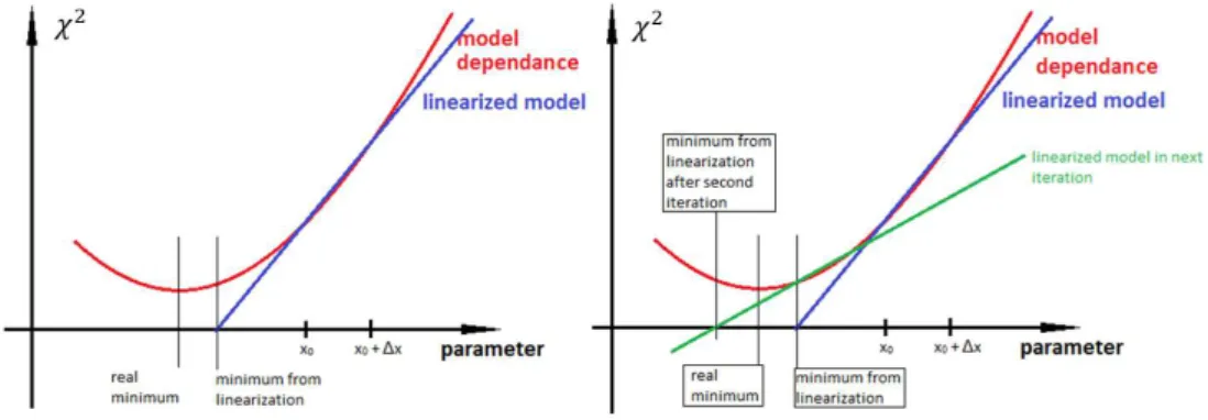
While using this method helped us quickly set up the fitting framework, the limitations soon became obvious. First, the linear approximation tends to be unstable close to the minimum. That is because near the minimum, the linearized model can cause larger changes of χ2 than the actual changes from the model (see Figure 3).
Depending on the shape of the function, this may cause the method to indefinitely jump around the minimum, resulting in a lack of convergence.
Figure 3. One-dimensional example of how linearization of parameter dependence of model affects fitting parameters to the data. Minimum of χ2
test between experimental data and model predictions is shifted from real minimum to minimum from linearization. In the se-cond iteration (right-hand plot), the result will drastically change the first derivative for the
third iteration.
This can be alleviated by calculating the result in one additional point for each parameter to calculate the estimation of the second derivative. Then, by requiring that the part dependent on the second derivative in the Taylor expansion is much smaller than linear terms8, we can estimate a region in which the linear approximation of
8The work on evaluating the stopping condition has not been completed. It will be a useful step
this parameter is valid9. Narrowing the range of the next step to this region helps
stabilize the model, making it easy to get very good results with less iterations. On the other hand narrowing strongly the steps in parameter space close to the minimum, makes it extremely slow to converge. The second derivative can also be used to estimate the distance to the minimum and to define a stopping condition. Also, if additional samples are computed on separate cores, these calculations do not affect the computation time of a single iteration.
2.5. Results and applications
Development of this method was postponed to complete work on the semi-analytic method, which is described in the following sections. This decision was made to take advantage of the unfolded data fromBaBar, which does not benefit from the increased versatility of the C template method. Because of this, further improvements were not added to this method.
Comparison of the best results obtained using this method (without theσ reso-nance in the decay mechanisms, see the beginning of Section 2.3 and Section 3.1) to the data, can be seen in Figure 4. The current version of this method takes about two weeks to converge.
Figure 4. The results of the fits compared to the data. The differential decay width of the channel τ−
→ π−π−π+ντ versus the invariant mass distributions is shown. BaBar
expe-riment measurements (black points), results from the RχL (blue line) and the CLEO tune (red dashed line) are overlaid. Ratio of new RχL prediction to the data is at the bottom.
The goodness-of-fit for these results isχ2
/ndf= 55264/401.
This approach has proven to be invaluable in understanding the behavior of the fitted model and helped us estimate the potential of the model to represent the data. We have chosen to develop this method because of its vast applicability in different
9Alternatively, we could introduce an adaptive step size. Using first or second derivatives, we
aspects of validating a physics model. For example, it can be used to fit data where experimental cuts have been applied. It can also be used with a re-weighting process, as described in Section 2.1, where each event is attributed with a weight dependent on the model used. This allows us to process an previously-generated event sample and analyze its characteristics using a different model.
These applications will definitely be useful in future analysis. However, to com-plete this analysis, we had to be able to thoroughly verify the model and the fitting framework itself. However, due to inefficiency of this method, some steps of the va-lidation procedures could not be performed with satisfying results. For example, the random scan of parameter space mentioned in Section 4.3.2, which allows us to find a starting point closer to the minimum, significantly improved the efficiency of the fitting algorithm. To obtain more-precise results and to be able to validate them, a new approach had to be taken. This required changes both to the fitting framework and to the physics model itself.
Let us stress that at present, we use the gradient method mainly as a cross-check for the semi-analytical method described in Section 3, as this is our default method for the numerical results of the physics interest. This is why some of the aspects of the gradient method (if it was used to obtain physics results) are not fully explored. We will return to this aspect of our work in the future, once the gradient method will be central for the precision fitting.
3. Semi-analytic method
3.1. Improving the physics model
With the availability of unfolded data from the experiments, an alternative strategy using semi-analytic methods was developed. A set of semi-analytic distributions10had
been prepared that correspond to the data distributions available to us. This required a substantial effort on the experimental side as well. Using these, we were able to make a direct comparison with the data. While these distributions cannot be used in the manner described in Section 2.5, they allowed for more efficient techniques due to the efforts mentioned above.
We have also included the final state Coulomb interactions. The estimated effect of this interaction on the results was relatively low; but for completeness, it had to be tested [10].
As mentioned in [15] and seen on Figure 4 (middle plot), the main concern in the case of the modeled process was the low-mass region, which both the oldCLEOmodel and the new χmodel have problems representing. Because our model was unable to describe that region, we added the low-mass scalarσresonance [12], which has been used in previous experiments to describe the low mass region, to our model. While the
10These distributions use analytical integration methods supported with numerical integration of
σresonance is not well-defined by the theory, may not be a true resonance, and is not part of the RχL scheme, it has been added in a way that does not conflict with the RχL scheme (see [10], eq. (3)–(7)). The impact of theσresonance was tested in [10]. Implementing changes in the model (contribution of the σ state) significantly improved the agreement with the data. A new comparison of our starting point to the data has been shown in Figure 5. One can see that the agreement of the starting point is already better than the best result of our previous approach, especially when analyzing the ratio of the new model to the data from the middle plot.
Figure 5. Starting point for the new fitting method, after applying improvements to the theoretical model. The goodness-of-fit for these results isχ2
/ndf = 32413/401. See caption of Figure 4 for description of the plots.
3.2. Improving the fitting framework
Parallel to the work on the physics model, the fitting framework has been improved as well. Switching from the MC simulation to semi-analytic distributions proved to be very effective. Just by using these functions instead of the full MC simulation we have gained more than a factor of 200. On a single core, without any optimizations, a single step took about one minute to compute11. And yet, there was still more room
for improvement.
The new performance bottleneck was the three-dimensional integration. The previously-used 16-point Gaussian integration method was changed from a variable-step-size to a constant-variable-step-size approach. Even though the first approach is more sophisticated, the second is better suited for fitting functions where even a small change of integrals can be significant. The fitting algorithm internally calculates the derivatives of the distributions with respect to all model parameters. The variable-step-size integration creates artificial discontinuities in the fitting function at points where step size changes. Such artifacts were problematic for the fitting procedure when near the minimum; therefore, we decided to use a more-stable method at a very small precision cost.
11At that moment, we were not taking into account the computation of the width of the resonance
To further smoothen the integrand and improve convergence, a change of inte-gration variables was introduced according to the following scheme:
Z x2
x1
f(x)dx=
Z 1
0
g′(t)f(g(t))dt,
where: y1= arc tg x
1−A2
AB
, y2= arc tg x
2−A2
AB
,
x=g(t) =A2+ABtg(y1+t(y2−y1)),
g′(t) =A2+(g(t)−A2)2+A2B2
AB .
(4)
This changes the integrated variable from x to g(t), introducing two adjustable parameters (A,B). This setup is commonly used to optimize the integration of func-tions describing resonances in particle physics, where parameter A is the resonance peak and B is the resonance width. In our calculations, we have chosen parameter A close to peak of ρ resonance [12] (which can be seen in Figure 5, middle plot) and decided that parameter B should not be too narrow, to account for the width of the a1 resonance (seen in Figure 5, right-hand plot). Based on the results from our
benchmark tests, we have chosen A = 0.77, B= 1.8 without further consideration of possibly more optimal choices.
The change of variables and stability of semi-analytical functions allowed us to reduce the number of steps of the integration algorithm. While the variable-step-size integration could take from 6 to 18 steps for the selected integration domain, we have benchmarked several choices of constant-step-size approach.It turned out that the precision of calculations did not improve past the 3 steps. We decided to use 2 steps, as the difference between 2 and 3 was not significant. Applying these changes brought a gain of speed close to a factor of ten.
3.3. Parallelization
Building our fitting environment around the semi-analytical distributions allowed for an easy way to introduce parallelization. At this point, the only time-consuming operation was 3-dimensional integration. This job can easily be sub-divided into as many parts as needed, and each task can be computed independently. This makes parallelization straightforward; the only restriction in this manner is the technology used for this purpose.
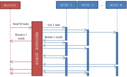
Since part of the tests will have to be done by our collaborator on a computing cluster with unknown support for parallel computing, we had to prepare a method that would be as portable as possible. Fortunately, the Inter-Process Communication (IPC) methods of UNIX systems proved to be more than enough for this task. Therefore, we decided to base our algorithm on message queues.
any other IPC methods12 (see Figure 6). Since the operating system takes care of
cashing sent messages and distributing them to the first node that is ready to receive the message, this simplifies the whole process down to few points that have to be taken into account when writing the master program and the computing nodes.
Figure 6. Diagram of communication between master program and computing nodes using message queue. Note that both master program and computing nodes can send and receive messages in an asynchronic way. Master program does not have to actively wait for nodes to
finish their computations.
Our algorithms works as follows:
1. The master program divides the job into smaller tasks and sends a complete list of tasks to the queue, creating a pool of tasks for computing nodes. The ordering of the tasks is irrelevant.
2. Computing nodes wait for a message to appear in the queue, then proceed to compute the requested task and send the result back to the queue with proper ID for the master program to receive them.
3. The master program waits for a message with proper ID and gathers the results. 4. Computation ends when the number of messages received equals the number of
messages sent.
This algorithm requires few things to take into consideration: 1. The master program must be prepared to receive data in any order.
2. A node that failed mid-computation (for any reason) will not return any results. A time-out must be put in place to decide when the master program has to re-send tasks that have not been computed.
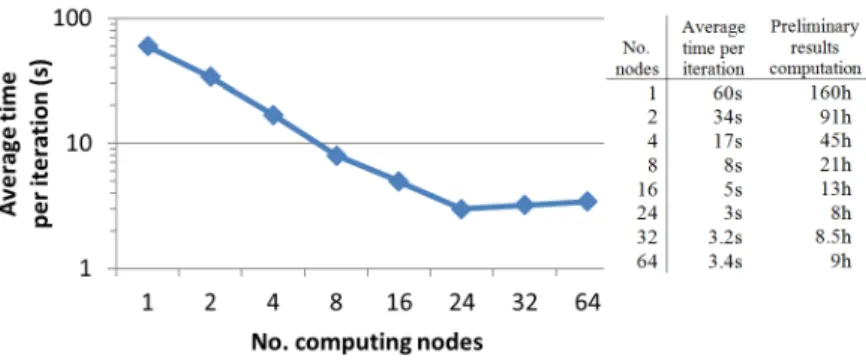
Both issues are easy to resolve. With this algorithm in place, the number of computing nodes can be freely adjusted, allowing us to optimize the resources used versus computation time. Our tests showed a linear decrease in computation time with the increase of cores used for computation up to 24 cores. Above this threshold, communication becomes the main factor that slows down the progress. This could be mitigated by increasing the size of the tasks sent to one node, but we decided against further optimization as the computing time was satisfactory at this point.
3.4. Approximating the width of the
a
1resonance
As mentioned in Section 2.1, one of the key components of the model is the a1
reso-nance width. Our first attempts used the same approximation as in the MC approach, where the width of the a1 resonance is calculated only at the starting point of the
fitting procedure. However, the lack of a proper recalculation of this resonance turned out to greatly influence the results. A fitting procedure that relies ona1width
calcu-lated only once ends in a minimum completely off the global minimum found when this width is properly recalculated for each point in parameter space.
Having wrong values of the a1 width can skew the result, creating a minimum
heavily correlated with a starting point for which the width was generated. This meant that we had to include thea1 width in our calculations.
Since the calculation time ofa1 width significantly dominates the whole
compu-tation time, we decided to introduce an old method in use since 1992 to optimize the fitting framework (used to approximate thea1 width). This approximation, based on
a general knowledge of the shape of a1 width distribution, uses a piecewise function
built upon sets of polynomials to interpolate thea1width. It is parameterized by
cal-culating the width in as few as 8 points. This approximation has been tested to show that it introduces deviations from the precise calculations less than 7% for low-mass region and less than 1% for the most important region.
Later on, when the parallelized calculation had been introduced, we were able to easily incorporate the precise calculations into the project. These calculations, however, still took the majority of computation time, so we left an approximated function as an option that can be used to quickly obtain preliminary results, as it may be important in future applications.
4. Results
4.1. Final results of the fits
Figure 7 shows the result of the fits using the semi-analytical method described in Section 3 compared to the data and results of the CLEO parameterization used so far by the experiments. The goodness of the fit is quantified by χ2/ndf = 6658/401.
be addressed. These comparisons can serve as a starting point for future precision studies ofτ decays [13].
Figure 7.Final results of the fits. The goodness-of-fit for these results isχ2
/ndf= 6658/401. See caption of Figure 4 for description of the plots.
Table 1
Final results of the fits – parameter values and their ranges. The approximate uncertainty estimates from theMINUITare 0.4 forRσ, 0.13 forM
ρ′ and below 10
−2
for rest of the para-meters.
Since the focus of this paper is on the technical aspects of this project, we refer the reader to [10] for physics-related results. Instead, we will focus on performance results and validation process of the fitting framework in this section.
4.2. Performance
Improvements to the fitting framework reduced computation time drastically. On a single 2.8GHz core with all approximations in place, a single iteration takes about one minute to complete. This computation time scales linearly with amount of cores used for computation, up to 24 cores; in this case, it takes about 3 seconds to compute one iteration.
complete a single iteration. Preliminary results were available in 2.5 hours. However, its use turned out to be impractical, as one 64-core job waited far longer in the computing cluster queue than three 24-core jobs.
The precise computation of the width of thea1resonance increases computation
time by a factor of two. This reduces the χ2 only by about 10%. In the final steps,
we removed the approximation of using only the value at the bin center and replaced it with the correct treatment, where we integrate over the bin width. This makes the χ2smaller by another 5–6% at a cost of 3 to 5 times slower computation. When both
options are included and fits are performed from the point calculated without these improvements, theχ2is reduced yet again by 5% to 6%. Ultimately, the final result on
24-core machine takes 2 to 3 days to complete, as compared to two weeks on a 32-core machine for a Monte-Carlo approach.
Figure 8.Scalability of the parallel distribution method using one message queue, one master program and sending one task per message. Above 24 cores, there is no improvement observed as the communication between computing nodes and master program starts domination over
the computation time gain.
The ability to obtain preliminary results within one day and to produce precise results within three days gave us an opportunity to test a number of different fitting strategies and to thoroughly validate our approach. This also allowed us to perform advanced systematics studies in a reasonable time frame.
4.3. Validating the results
Having an efficient fitting framework at our disposal, we could dedicate more time to the validation process, which is a crucial step in the fitting process. Our validation process consisted of asserting statistical errors and correlation coefficients between the parameters, verifying that the result we have found is a global minimum and performing studies of the systematics errors.
4.3.1. Statistical errors and correlations
of 2nd derivatives and inverts it. The results show strong correlations between four parameters of the model indicating that the model has more free parameters than can be determined by the data. This is something that could have been expected and this issue was addressed in more details in [10].
4.3.2. Convergence of the fitting procedure
The purpose of the convergence test is to verify how the fitting procedure behaves when starting from different points. This test helps to verify that the minimum found by the fitting procedure is, in fact, a global minimum. It was done in the following steps:
•Random scan of parameters space. Since precision was of a lesser concern at
this step, we have used all available approximations yielding a sample of 12,000 distinct parameter sets per hour using 240 cores.
•Having gathered more than 200k samples, we began searching for any patterns
that could help us narrow down the region in parameter space where there is a larger chance of finding a global minimum.
•We choose a 1k sample of distributions for distinct parameter sets with the lowest
χ2 and choose 20 points from this parameter sets in a way that maximized the
distance between these points.
•We perform fits to the data using these 20 configurations as starting point for
the independent fits.
The results have shown that more than 50% of the fits converge to the minimum shown as our final result. In other cases, either the minimization process fails due to the number of parameters being at their limit, or they converge to a local minima of distinguishably higherχ2 (by a factor of 10 or more). This indicates that our model
has several local minima. At the same time, it points out that there is a good chance of our result being a global minimum.
4.3.3. Systematic uncertainties
We have estimated the systematic uncertainties using toy MC studies. Every toy MC sample has been generated under the Gaussian assumption using the Cholesky decomposition on systematic covariance matrix provided by the BaBar experiment to include the correlations between bins of the data histograms. The fit was re-run for one hundred samples to estimate the systematic uncertainties. It took less than a week using 320 cores to complete this step (which would be near to impossible to complete using MC approach).
5. Summary and outlook
We have presented a fitting strategy used for comparing RχL currents for τ →
π−π−π+ν
τ with experimental data. The resulting improvements to theτ decays MC
We have presented two methods; one based on an MC simulation and the other based on semi-analytical distributions. While the first approach is significantly slower, it can be used in cases where analytic solutions are not available, such as presence of experimental cuts in data on multi-dimensional distributions.
We have presented improvements both to the theoretical model and to the fitting framework that significantly reduce computation time: from 2 weeks for the MC-based method to 2–3 days for method MC-based on semi-analytic distributions. We have presented approximations introduced to the computations that allowed us to compute preliminary results within 8 hours. We have also introduced a scalable parallelization algorithm based on basic Inter-Process Communication methods of UNIX operating systems.
In the future, we are planning to use this framework to test the model against 2-dimensional data forτ→π−π−π+ντ and for fits of τ→K−π−K+ντ decay channel.
Fits for other decay modes will follow. As a final step of our work, we are planning to complete a model-independent fitting framework incorporating strategies presented in this paper with the ability to expand its application to multi-dimensional data and new fitting strategies.
Acknowledgements
We thank Ian M. Nugent for his collaboration on this project. Part of the computations were supported in part by PL-Grid Infrastructure(http://plgrid.pl/)and were per-formed on ACK Cyfronet computing cluster(http://www.cyfronet.krakow.pl/).
This project was partially financed from funds of Foundation of Polish Scien-ce, grant POMOST/2013-7/12 and funds of Polish National Science Centre under decisions DEC-2011/03/B/ST2/00107. This research was supported in part by the Research Executive Agency (REA) of the European Union under the rant Agreement PITNGA2012316704 (HiggsTools). P.R. acknowledges funding from CONACYT and DGAPA through project PAPIIT IN106913.
References
[1] Actis S., et al.: Quest for precision in hadronic cross sections at low energy: Monte Carlo tools vs. experimental data. Eur. Phys. J., vol. C66, pp. 585–686, 2010.
http://dx.doi.org/10.1140/epjc/s10052-010-1251-4.
[2] Antcheva I., Ballintijn M., Bellenot B., Biskup M., Brun R., et al.: ROOT: A C++ framework for petabyte data storage, statistical analysis and visualization. Com-put. Phys. Commun., vol. 180, pp. 2499–2512, 2009.
http://dx.doi.org/10.1016/j.cpc.2009.08.005.
[3] Asner D., et al.: Hadronic structure in the decayτ→π−π0π0and the sign of the tau-neutrino helicity. Phys. Rev., vol. D61, p. 012002, 2000.
http://dx.doi.org/10.1103/PhysRevD.61.012002.
[5] Banerjee S., Kalinowski J., Kotlarski W., Przedzinski T., Was Z.: Ascertaining the spin for new resonances decaying into tau+ tau- at Hadron Colliders. Eur. Phys. J., vol. C73, p. 2313, 2013.
http://dx.doi.org/10.1140/epjc/s10052-013-2313-1.
[6] Ecker G., Gasser J., Pich A., de Rafael E.: The Role of Resonances in Chiral Perturbation Theory. Nucl. Phys., vol. B321, p. 311, 1989.
http://dx.doi.org/10.1016/0550-3213(89)90346-5.
[7] Jadach S., Kuhn J. H., Was Z.: TAUOLA: A Library of Monte Carlo programs to simulate decays of polarized tau leptons. Comput. Phys. Commun., vol. 64, pp. 275–299, 1990. http://dx.doi.org/10.1016/0010-4655(91)90038-M. [8] James F., Roos M.: Minuit: A System for Function Minimization and Analysis
of the Parameter Errors and Correlations. Comput. Phys. Commun., vol. 10, pp. 343–367, 1975. http://dx.doi.org/10.1016/0010-4655(75)90039-9. [9] Kubota Y., et al.: The CLEO-II detector. Nucl. Instrum. Meth., vol. A320, pp.
66–113, 1992. http://dx.doi.org/10.1016/0168-9002(92)90770-5.
[10] Nugent I., Przedzinski T., Roig P., Shekhovtsova O., Was Z.: Resonance chiral Lagrangian currents and experimental data forτ−
→π−π−π+ντ.Phys. Rev., vol.
D88(9), p. 093012, 2013. http://dx.doi.org/10.1103/PhysRevD.88.093012. [11] Nugent I. M. [BaBar Collaboration]: Invariant mass spectra ofτ−
→h−h−h+ντ
decays, Nucl. Phys. Proc. Suppl. 253–255, 38 (2014) [arXiv:1301.7105 [hep-ex]]. [12] Olive K., et al.: Review of Particle Physics. Chin. Phys., vol. C38, p. 090001,
2014. http://dx.doi.org/10.1088/1674-1137/38/9/090001.
[13] Pich A.: Precision Tau Physics. Prog. Part. Nucl. Phys., vol. 75, pp. 41–85, 2014.
http://dx.doi.org/10.1016/j.ppnp.2013.11.002.
[14] Przedzinski T.: Test of influence of retabulation method on fitting convergence, 2011.
[15] Shekhovtsova O., Nugent I., Przedzinski T., Roig P., Was Z.: RChL currents in Tauola: implementation and fit parameters. Nucl. Phys. Proc. Suppl., 253–255, pp. 73–76, 2014.
UAB-FT-727http://dx.doi.org/10.1016/j.nuclphysbps.2014.09.018
[16] Shekhovtsova O., Przedzinski T., Roig P., Was Z.: Resonance chiral Lagrangian currents andτ decay Monte Carlo. Phys. Rev., vol. D86, p. 113008, 2012.
http://dx.doi.org/10.1103/PhysRevD.86.113008.
[17] ’t Hooft G.: A Planar Diagram Theory for Strong Interactions. Nucl. Phys., vol. B72, p. 461, 1974. http://dx.doi.org/10.1016/0550-3213(74)90154-0. [18] Verkerke W., Kirkby D. P.: The RooFit toolkit for data modeling. eConf,
vol. C0303241, p. MOLT007, 2003,
[19] Witten E.: Baryons in the 1/n Expansion. Nucl. Phys., vol. B160, p. 57, 1979.
Affiliations
Tomasz Przedziński
The Faculty of Physics, Astronomy and Applied Computer Science, Jagellonian University, Krakow, Poland,[email protected]
Pablo Roig
Departamento de F´isica, Centro de Investigacion y de Estudios Avanzados del Instituto Polit´ecnico Nacional, Apartado Postal 14-740, 07000 M´exico D. F. 01000, M´exico
Olga Shekhovtsova
Kharkov Institute of Physics and Technology 61108, Akademicheskaya,1, Kharkov, Ukraine. Institute of Nuclear Physics, PAN, Krakow, Poland
Zbigniew Wąs
Institute of Nuclear Physics, PAN, Krakow, Poland
Jakub Zaremba
Institute of Nuclear Physics, PAN, Krakow, Poland
Received: 4.07.2014
Revised: 30.10.2014