Abstract—Without assuming the symmetry of the connected
matrix and the boundedness or monotonicity of the nonlinear activation functions, some new sufficient criterions are obtained for the asymptotic stability in the large for a class of neural networks. These criterions are applied easily and widely too.
Index Terms—Asymptotic stability in the large,
Boundedness, Monotonicity, Hopfield Neural network
I. INTRODUCTION
The Hopfield neural network (HNN [1]–[3]) theory and its application are extensively discussed in literature, for example, [3]–[17], [19], [21]–[29] and the references cited therein. M. Ghatee and M. Niksirat [7] dealt with maximum cut problem on a graph with fuzzy edges. An adaptive Hopfield neural network with modern simulated annealing cooling schedule was proposed to solve the problem. Its efficiency was tested for some simulated benchmark examples. M. Sheikhan and E. Hemmati [13] explored the use of Hopfield neural network as a path set selection algorithm. The authors used link expiration time between two nodes to estimate link reliability. In this method, node-disjoint and link-disjoint path sets can be found simultaneously with route discovery algorithm. Simulation results showed that the proposed protocol can find path sets with higher reliability comparing to other recently proposed algorithms. In monograph [19] some sufficient conditions were obtained for the stability of the HNN. In [29] a new 5 × 7 optimized FLC-coupled HNN maximum tracking technique was designed. A HNN was used to tune the fuzzy membership function routinely. Entire components of a PV array, a DC–DC buck-boost zeta converter and a designed MPP tracking controller were implemented in a Matlab–Simulink tool to validate the HNN. The results validated the effectiveness and execution of the HNN using the optimized fuzzy system. The designed system was successfully tested on an experimental prototype.
As we know, determining the stability of the equilibrium points is essential for the HNN and its application [4], [5], [12], [17], [19]. It is commonly assumed that the connected matrix is symmetrical or the nonlinear activation functions are monotonously non-decreasing or bounded ([3]–[16] etc.) in the stability criterions for HNN.
In the paper, we prove some new sufficient criterions of asymptotic stability in the large for the HNN by means of analysis and calculation method without assuming the
Manuscript received February 26, 2015. This work was supported by China National Natural Science Foundation Grant No. 11171014.
Jiemin Zhao is with the College of Information Technology, Department of Applied Mathematics and Physics, Beijing Union University, Beijing 100101, China (Tel: 86-010-64900271; fax: 86-010-64900217; e-mail: [email protected]).
symmetry of the connected matrix, and the boundedness [20], or the monotonicity of the nonlinear activation functions.
This paper is arranged as follow. In section 2, we state the main results. In section 3, we give the proofs of theorems. In section 4, we briefly discuss our conclusion.
II.MAIN RESULTS
Consider the following Hopfield neural network
1 1
( ) ( ) ,
( ), 1, 2, , , n
i i
i i j j i
j i
i i i
d u t u t
C w V I
d t R
u g V i n
(1)
where w Vi j i represents the electrical current input to cell
idue to the present potential of cell j, and wi j is thus the synapse efficacy. Linear summing of inputs is assumed. Ii is any other (fixed) input current to neuron i. uiis the neural voltages. Ri is the resistances. Ci is the capacitance [1]–[4].
We know that HNN there exists equilibrium point [19]. Suppose u ( , , , )u u1 2 un T
is an equilibrium point of system (1). Let x u u( , , ,x x1 2 xn) ,T then system (1) can be rewritten as following equivalent system [19]
1 ( ), 1, 2, , ,
(0) 0, 1, 2, , , n i i
i i j j j j
i j
d x x
C w f x i n
dt R
f j n
(2)
where ( )fj xj gj(xj uj) g uj( ).j
Define nsgn x ai, i jas follows:
1, 0,
( 1, 2, , ), 1, 0,
( , 1, 2, , ).
i i
i i j i i j i
x
nsgn x i n x
a R w nsgn x i j n
The following Theorem 1 through 5 do not need the symmetry of the connected matrix or the boundedness and the monotonicity of the nonlinear activation functions.
Theorem 1. If
1
( ) n | | 0, 1, 2, , ,
j j i j j j
i
f x a x for x j n
(3)then system (2) is asymptotically stable in the large. Theorem 2. If
1
| ( ) |j j n i| i j| | | forj j 0, 1, 2, , , i
f x R w x x j n
then system (2) is asymptotically stable in the large.
Theorem 3. If | ( ) |f xj j j (j const.0) and
A Note on Hopfield Neural Network Stability
1
| | 1, 1, 2, , , n
j i i j i
R w j n
then system (2) is asymptotically stable in the large.
Theorem 4. If | ( ) |fj xj Kj| |xj (Kj const.0) and
1
| | 1, 1, 2, , , n
j i i j i
K R w j n
then
s
ystem (2) is asymptotically stable in the large. Theorem 5. If| ( )f uj f vj( ) |L uj| v| (u v, R L, j const.0) and
1
| | 1, 1, 2, , , n
j i i j i
L R w j n
then system (2) is asymptotically stable in the large . For the HNN, it is commonly assumed that the connected matrix is symmetrical and the hyperbolic tangent function tanhcxis taken as activation function ( [7], [16] etc.). We have no requirement for the symmetry of the connected matrix in the following Theorem 6 and Theorem 7.
Theorem 6. Suppose
1
| | 1, 1, 2, , n
i i j i
R w j n
.1) If
1
( ) tan , , , 0 1,
j j j j j j j j j
f x b c x b c const b c then system (2) is asymptotically stable in the large.
2) If fj( )xj bjtanhc xj j,then system (2) is asymptotically stable in the large.
3) If fj( )xj bjsinh 1c xj j,
then system (2) is
asymptotically stable in the large.
Theorem 7. If ( ) | 1| | 1|
2
j j
j j
x x
f x and
1
| | 1, 1, 2, , , n
i i j i
R w j n
then system (2) is asymptotically stable in the large. III. PROOF OF THE THEOREMS
Proof of the Theorem 1
We need following Lemma in the proof of Theorem 1.
Lemma. Suppose that the functions fi j( )xj are continuous and satisfy the conditions such that the uniqueness theorem of solutions holds for the system
1
( ), 1, 2, , , (0) 0
n i
i j j i j
j
d x
f x i n f dt
. (4)We also suppose, that there are numbers
0, 0 (1 )
i i
a b i n
such that
1
( ) ( ) 0 n
i i i j j i
x f x
for xj 0 (1 j n) (5)where
, 0,
( )
, 0,
i i i i
i i
a x
x
b x
(6) then the zero solution of (4) is asymptotically stable in the large [18].
Proof of the Lemma. To prove the Lemma we use the comparison function
1 1
( ) n ( ) [ ( , , ) ],T
i i i n
i
V x x x x x x
(7)which satisfies a Lipschitz condition in n
R . We have
1
1 1
1
| ( ) ( ) | | ( ) ( ) |
Max ( , ) | |
Max ( , , ) | |. n
i i i i i i i
n
i i i i i
n
n i i
i
V x V x x x x x
a b x x
a b x x
Let
Min( , ),i i Max( , )i i
i a b i a b
and 2 21
1
| | ( n i ) ,
i
x x
then| ( )V x V x( ) |√n|xx|
Specially V x( )√n| |x . In addition,
1 1
( ) n | ( ) || |i i i n | |i | |
i i
V x x x x x
as | |x . That implies that Vis positive-definite and
“infinitely large”.
Now we consider an arbitrary (non-trivial) solution of (4)
( ; , )
x t [ ( ; , )x 0].
Firstly, we prove that the comparison function V , i.e.,
( )t V x t( ( ; , ))
is strict decreasing along this solution. It is enough to show
( )t ( )V( )
for t (8)
as long as the solution exists. The existence of solution for
t
then follows from the estimate. By
1
( ) ( ), 1, 2, ,
n i
i j j i j
t
d x
f f i n dt
we have
( ; , )
lim i i ( ),
i t
x t
f t
So, for any given positive number0, we can assign a positive number ( ) 0 such that for t ,
the following inequalities hold
( ( ) )( ) ( ; , ) ( ( ) )( ).
i fi t x ti i fi t
In case ofx ti( ; , ) 0 , we have
( ) ( ) ( )( ( ) )( )
i x xi i i xi i i xi fi t . And in case of x ti( ; , ) 0 , we have
( ) ( ) ( )( ( ) )( )
( ) ( ) ( )( ( ) )( ) i x xi i i xi i i xi fi i t , Therefore
1 , 1
( ) ( ) ( ) ( ) ( )
( ), [ , ].
n n
i i i i i i j j
i i j
t x t x f
n t t
Choosing so that the signs of every non-zero component i
and the corresponding component ( ; , )x ti coincide (that is, ( )i xi i( )i for i 0), we obtain
( ) ( ) ( ) { ( ) ( )j j j j j j
t t f
( ) ( )} ( ),
( ) ( ) ( ) ( ) ( ) ( )
i i i j j i j
j j j
x f n t
t t n t
for all jwith j 0 and sufficiently small.
If there is a time 2 such that 2
( ) ( ), ( )t ( )
for t 2,
then the function ( )t attains its minimum in ( , ) 2 , at 1,
say.
Denoting 1x( ; , ), 1 x t( ; , ) 1 1 x t( ; , ) , we
can prove similarly
1 1 1 1
( )t V x t( ( ; , )) ( )V( )
for 1 t 1 1. But this is a contradiction, so (8) is true.
Because the function
( )t V x t( ( ; , ))
for t
is decreasing, it follows immediately that x0 is a stable
solution, and
1 1
| ( ; , ) |x t ( )t ( ) n | | (t ),
√
for
| | ( ) .
n
√
Hence every solution x t( ; , ) is bounded for t, and the following limit exists
0
lim ( ( ; , )) 0
tV x t V .
Since the solution has a non-empty - limit set, there also exists an - limit trajectory x t( ),0 and for every fixed t we
can find a monotone increasing divergent sequence {tk} such that
0
lim ( ; , )k ( )
kx t x t
[and lim ( ( ; , ))kV x tk V x t( ( ))0 ].
Consequently, we have for all t
0 0
( ( )) ,
V x t V
which shows that x t0( ) 0 and V00, because the comparison function decreases strictly along every non-trivial solution.
It follows immediately that
lim ( ; , ) 0
tx t This establishes the Lemma [18].
Using this Lemma, we can prove the Theorem 1. In fact, let
( )
i xi
be the piecewise continuous functions defined as following
, 0,
( ) i i, i 0, 1, 2, ,
i i
i i i
C R x
x i n
C R x
and the functions fi j( )xj defined by
1 2
1 1 1 1 2 2 2 2
1
1 1 1 1
( ) ( ), ( ) ( ), ,
( ) ( ), ( ) ( ),
i i
i i
i i
i i i i i
i i i i i i i i i i
i i i i
w w
f x f x f x f x
C C
w x w
f x f x f x f x
C C R C
1
1( 1) 1( 1), , ( ) ( ),
i i i n
i i i i i i n n n n
i i
w w
f x f x f x f x
C C
then
1 1 1 2 2 2 1 1 1
1 1 1
1 2
1 1 2 2
1 2
( ) ( ) ( ) ( ) ( ) ( )
( ) ( ) ( ) ( ) ( ) ( )
( ) ( ) ( ) ( )
j j j j j j j j j
j j j j j j j j j j n n n j j
j j
j j j j
x f x x f x x f x
x f x x f x x f x
w w
f x x f x x
C C
1
1 1 1
1
1 1 1
1 2
1 1 1 2 2 2
1 2
( ) ( ) ( ( ) ) ( )
( ) ( ) ( ) ( )
( ) ( )
j j j j j
j j j j j j j j
j j j j
j j n j
j j j j j j n n
j n
j j
j j j j
w w x
f x x f x x
C C C R
w w
f x x f x x
C C
w w
f x C R nsgn x f x C R nsgn x
C C
1
1 1 1
1
1
1 1 1
1
1 1 1 2 2 2
1 1 1 1 1 1
( ) ( ( ) )
( )
( ) (
j j j j j
j j j j j j j
j j j j
j j n j
j j j j j j j j
j n
j j n n n j j
j j j j j j j j j j j j
w w x
f x C R nsgn x f x
C C C R
w w
C R nsgn x f x C R nsgn x
C C
f x C R nsgn x R w nsgn x R w nsgn x
R w nsgn x R w nsgn x R w nsgn x
1 1 1
2 2 2 1 1 1
1 1 1
1 2 1 1
) ( ) (
) ( )
( ) ( ) .
n n j n j j j j j
j j j j j j j j j
j j j j n n j n j j j
j j j j j j j j n j j j j R w nsgn x f x x nsgn x R w nsgn x
R w nsgn x R w nsgn x R w nsgn x
R w nsgn x R w nsgn x f x x
a a a a a a f x x
If
1 2 1 1
( ) ( )
0 for 0 ( 1, 2, , ),
j j j j j j j j n j j j j j
a a a a a a f x x
x j n
then the Hopfield neural network (2) is asymptotically stable in the large.This ends the proof of the Theorem 1.
Proof of the Theorem 2
If
1
| ( ) |j j n i | i j| | | forj j 0, 1, 2, , ,
i
f x R w x x j n
then1
1
( )
| ( ) | | | | | for 0, 1, 2, , .
n j j i j
i n
j j i i j j j
i
f x a
f x R w x x j n
Proof of the Theorem 3
If | ( ) |f xj j j (j const.0), then
| ( ) | | ( ) (0) |
| ( )( 0) | | ( ) | | |,
j j j j j
j j j j j j
f x f x f
f x x f x
where belongs to (0, )xj for xj 0 or belongs to
( , 0)xj for xj 0. So,
1 1
( ) | | | |
| | for 0, 1, 2, , .
n n
j j i j j j i i j
i i
j j
f x a x R w
x x j n
The system (2) is asymptotically stable in the large by the Theorem 1. This ends the proof of theorem 3.
Proof of the Theorem 4
If | ( ) |f xj j Kj| |xj (Kj const.0) and 1
| |
n j i i j
i
K R w
1, 1, 2, , ,j n
then
1 1
( ) | | | |
| | for 0, 1, 2, , .
n n
j j i j j j i i j
i i
j j
f x a K x R w
x x j n
This establishes the theorem 4 by the theorem 1.
Proof of the Theorem 5
If the function f xj( )j satisfies the Lipschitz condition, and
1
| | 1, 1, 2, , ,
n j i i j
i
L R w j n
thenall of the conditions of theorem 4 are satisfied. Therefore, the system (2) is asymptotically stable in the large. The proof of the Theorem 5 is completed.
Proof of the Theorem 6
1) Let
1
( ) ( ) tan for 0, 1, 2, , .
j j j j j j j j j
j
g x x f x x b c x x j n
If b cj j (0, 1], then
2 2
2
( ) 1
1 ( ) ( ) (1 )
0 for 0, 1, 2, , , 1 ( )
j j j j
j j j
j j j j
j j j
b c d
g x
d x c x c x b c
x j n c x
and gj(0) 0. Consequently we have
( ) 0 for 0, 1, 2, , .
j j j j
x f x x j n
Therefore,
1
1 1 1
( ) | tan | | | | | | | | | for 0, 1, 2, , .
n n n
j j i j j j j i j j i i j
i i i
j j
f x a b c x a x R w x x j n
By the theorem 1, the system (2) is asymptotically stable in the large.
2) Let
( ) ( ) tanh for 0, 1, 2, , .
j j j j j j j j j j
h x x f x x b c x x j n
We have
2 2
( ) 1 sech 1 sech 0 1 0,
j j j j j j j j j j
j
d
h x b c c x b c b c d x
and hj(0) 0. Therefore,
tanh 0 for 0, 1, 2, , .
j j j j j
x b c x x j n
and
1 1 1
( ) | tanh | | | = | | | | | | for 0, 1, 2, , .
n n n
j j i j j j j i j j i i j
i i i
j j
f x a b c x a x R w x x j n
Hence, the system (2) is asymptotically stable in the large. 3) Let
1
( ) ( ) sinh for 0, 1, 2, , .
j j j j j j j j j
j
u x x f x x b c x x j n
then
2
2 2
1 ( )
( ) 1
1 ( ) 1 ( )
for 0, 1, 2, , ,
j j j j j j
j j
j j j j j
j
c x b c
b c d
u x
d x c x c x
x j n
and (0) 0.uj Consequently we have
( ) 0 for 0, 1, 2, , .
j j j j
x f x x j n
Therefore,
1 1
( ) | | | | | |
for 0, 1, 2, , .
n n
j j i j j i i j j
i i
j
f x a x R w x
x j n
It follows that the system (2) is asymptotically stable in the large. The proof of the theorem 6 is completed.
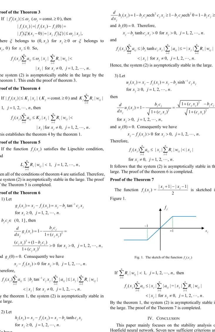
Proof of the Theorem 7
The function ( )f xj j =
| 1| | 1|
2
j j
x x
is sketched in Figure 1.
If 1
| | 1, 1, 2, , , n
i i j i
R w j n
then1 1 1
( ) | | | | = | | | |
| | for 0, 1, 2, , .
n n n
j j i j j i j j i i j
i i i
j j
f x a x a x R w
x x j n
By the theorem 1, the system (2) is asymptotically stable in the large. The proof of the Theorem 7 is completed.
IV. CONCLUSION
This paper mainly focuses on the stability analysis of Hopfield neural network. Seven new sufficient criterions are
j f
1
1 xj
given to guarantee the stability of Hopfield neural network. These conditions can be satisfied easily. And these results can be applied widely in more areas. The Hopfield model based neural network is used frenquently in practical applications.
ACKNOWLEDGMENT
The author would like to thank the anonymous reviewer, the Professor Cuiping Li, and the Professor Siqun Ye for their help, valuable comments and suggestions which helped me to improve the paper.
REFERENCES
[1] J. J. Hopfield, “Neural networks and physical systems with emergent collective computational abilities,” Proc. Natl. Acad. Sci. USA., vol. 79, pp. 2554–2558, April 1982.
[2] J. J. Hopfield and D.W. Tank, “Neural computation of decisions in optimization problems,” Biological Cybernetics, vol. 52, no. 3, pp. 141–152, 1985.
[3] J. J. Hopfield, “Neurons with graded response have collective computational properties like those of two-state neurons,” Proc. Natl. Acad. Sci. USA., vol. 81, no. 10, pp. 3088–3092, 1984.
[4] M. T. Hagan, H. B. Demuth and M. Beale, Neural Network Design. Boston: PWS Publishing, 1996.
[5] X. X. Liao, “Stability of Hopfield-type neural networks (I),” Science in China (Series A), vol. 38, no. 10, pp. 407–418, 1995.
[6] X. B. Liang and L. D. Wu, “Global exponential stability of Hopfield-type neural network and its applications,” Science in China (Series A), vol. 38, no. 6, pp. 757–768, 1995.
[7] M. Ghatee and M. Niksirat, “A Hopfield neural network applied to the fuzzy maximum cut problem under credibility measure,” Information Sciences, vol. 229, pp. 77–93, 2013.
[8] T. Xiong, B. L. Zhang, S. J. Chang, J. Y. Shen and Y. X. Zhang, “A multiple input-queued ATM switching fabric based on Hopfield neural network cell scheduling,” Acta physica sinica (in Chinese, English abstract), vol. 54, no. 5, pp. 2435–2440, May. 2005.
[9] S. Tayefi and A. Pazirandeh, “Evaluation of applying axial variation of enrichment distribution method and radial variation of enrichment distribution in VVER/1000 reactor using a Hopfield neural network to optimize fuel management,” Progress in Nuclear Energy, vol. 64, pp. 47–53, 2013.
[10] B. G. Tian, K. Gu and L. Jiang, “The calculation of the minimum entropy under the constraint based on the Hopfield network,” Acta mathematica scientia (Series A, in Chinese, English abstract), vol. 22, no.2, pp. 264–269, 2002.
[11] F. Wang, F. B. Wu and X. Huang, “Watermarking algorithms of wavelet image for Hopfield network with HVS combination,” Journal of xi’an university of science and technology (in Chinese, English abstract), vol. 33, no. 6, pp. 731–736, Nov. 2013.
[12] S. Xu, N. Ye, F. Zhu, S. S. Xu and L. L. Zhou, “Solving the stereo matching in disparity image space using the Hopfield neural network,” Journal of computer research and development (in Chinese, English abstract), vol. 50, no. 5, pp. 1021–1029, 2013.
[13] M. Sheikhan and E. Hemmati, “High reliable disjoint path set selection in mobile ad-hoc network using Hopfield neural network,” IET communications, Vol. 5, no. 11, pp. 1566–1576, 2011.
[14] Y. L. Zhou, L. Z. Song and H. J. Zhou, “Measurement of particle velocity in dilute phase based on PSO and Hopfield network matching,” CIESC Journal, Vol. 62, no. 2, pp. 348–354, Feb. 2011. [15] M. Atencia, G. Joya and F. Sandoval, “Identification of noisy
dynamical systems with parameter estimation based on Hopfield neural networks,” Neurocomputing, Vol. 121, pp. 14–24, 2013. [16] P. Yan and C. Zhang, Artificial Neural Networks and Evolutionary
Computing (in Chinese). Beijing: Tsinghua University Press, the
second edition, 2005, pp. 424–427.
[17] D. Jin and J. Peng, “A New Approach for Estimating the Attraction Domain for Hopfield–Type Neural Networks,” Neural Computation, Vol. 21, pp. 101–120, 2009.
[18] S. L. Li, “The global stability of the zero solution of
1
( ), 1, ,
n s
s j j j
d x
f x s n dt
and its applications,” Acta MathematicaSinica (in Chinese), Vol. 14, no. 3, pp. 353–366, 1964.
[19] S. M. Zhong, B. S. Liu, X. M. Wang and X. M. Fan, Stability Theory of Neural Networks (in Chinese). Beijing: Science Press, 2008, pp. 63–86.
[20] Jiemin Zhao, “A note on Razumikhin theorems in uniform ultimate boundedness,” Miskolc mathematical notes, Vol. 15, no. 1, pp. 239–254, 2014.
[21] J. Wang, X. H. Tang and X. J. Lin, “Recoverable Watermarking Algorithm for Text Authentication and Synonym Replacement Based on Hopfield Neural Network,” Pattern Recognition and Artificial Intelligence (in Chinese, English abstract), Vol. 28, No. 2, pp. 139–147, 2015.
[22] S. Tayefi and A. Pazirandeh, “Using Hopfield neural network to optimize fuel rod loading patterns in VVER/1000 reactor by applying axial variation of enrichment distribution,” APPLIED SOFT COMPUTING, Vol. 21, pp. 501–508, 2014.
[23] X. K. Ruan, Z. Z. Tang, Y. Z. Zhang, X. J. Chen and H. L. Chen, “Electrical blind detection of coherent optical communication signals using feedback-voltage-bias-type Hopfield neural network,” Infrared and Laser Engineering (in Chinese, English abstract), Vol. 44, No. 2, pp. 715–720, 2015.
[24] B. Sudarshan and R. Manjunatha, “Image storage and retrieval in graded memory,” International Journal of Advances in Engineering and Technology, Vol. 8, No. 1, pp. 2123–2128, 2015.
[25] T. Ganesan, P. Vasant and I. Elamvazuthi, “Hopfield neural networks approach for design optimization of hybrid power systems with multiple renewable energy sources in a fuzzy environment,” Journal of Intelligent and Fuzzy Systems, Vol. 26, No. 5, pp. 2143–2154, 2014. [26] G. Han, J. F. Qiao, H. G. Han and W. Chai, “Optimal control for
treatment process based on Hopfield neural network,” Control and Decision (in Chinese, English abstract), Vol. 29, No. 11, pp. 2085–2088, 2014.
[27] Y. Lou, Y. W. Zhao, Y. G. Song and W. F. Zhang, “Signal Recognition Technology of Sky Screen Based on Hopfield Neural Network,” ACTA ARMAMENTARII (in Chinese, English abstract), Vol. 35, No. 10, pp. 1587–1594, 2014.
[28] Hajar Asgari,Yousef S. Kavian and Ali Mahani, “A Systolic Architecture for Hopfield Neural Networks,” Procedia Technology, Vol. 17, pp. 736–741, 2014.