Simple stability conditions of linear discrete time systems with multiple delay

Vol. 7, No. 1, May 2010, 69-79

Simple Stability Conditions of Linear

Discrete Time Systems with Multiple Delay

Sreten B. Stojanovic

1

, Dragutin LJ. Debeljkovic

2

Abstract: In this paper we have established a new Lyapunov-Krasovskii method for linear discrete time systems with multiple time delay. Based on this method, two sufficient conditions for delay-independent asymptotic stability of the linear discrete time systems with multiple delays are derived in the shape of Lyapunov inequality. Numerical examples are presented to demonstrate the applicability of the present approach.

Keywords: Discrete time-delay systems, Lyapunov-Krasovskii method, Delay-independent stability, Liner matrix inequality.

1 Inotrduction

During the last three decades, the problem of stability analysis of time delay systems has received considerable attention and many papers dealing with this problem have appeared. In the literature, various stability techniques have been utilized to derive stability criteria for time delay systems by many researchers. The techniques can be grossly classified into two categories: frequency domain approach (which are suitable for systems with a small number of heterogeneous delays) and time-domain approach (for systems with a many heterogeneous delays).

The second approach is based on the comparison principle based techniques for functional differential equations [1, 2] or the Lyapunov stability approach with the Krasovskii and Razumikhin methods [3, 4]. In the past few years stability problems are thus reduced to one of finding solutions to Lyapunov [5] or Riccati equations [6] solving linear matrix inequalities (LMIs) [7] or analyzing eigenvalue distribution of appropriate finite-dimensional matrices [8].

It is well-known that the choice of an appropriate Lyapunov–Krasovskii functional is crucial for deriving stability conditions [9]. The general form of this functional leads to a complicated system of partial differential equations

1_{Faculty of Technology, University of Nis, Leskovac, Serbia, e-mail: [email protected]}

2_{Faculty of Mechanical Engineering, University of Belgrade, Belgrade, Serbia; E-mail: [email protected]}

[10]. Special forms of Lyapunov–Krasovskii functional lead to simpler delay-independent [2, 7, 9] and less conservative delay-dependent conditions [9, 11, 12]. In the past few years, there have been various approaches to reduce the conservatism of delay-dependent conditions by using new bounding for cross terms (Park’s and similarly inequalities) [2, 13] or choosing new Lyapunov–Krasovskii functional and model transformation. However, the model transformation may introduce additional dynamics [14]. In [15] it is shown that descriptor transformation leads to a system which is equivalent to the original one, does not depend on additional assumptions for stability of the transformed system and requires bounding of fewer cross-terms.

Since most physical systems evolve in continuous time, it is natural that theories for stability analysis are mainly developed for continuous-time. However, it is more reasonable that one should use a discrete-time approach for that purpose because the controller is usually implemented digitally. Despite this significance mentioned, less attention has been paid to discrete-time systems with delays [16-23, 25, 26]. It is mainly due to the fact that the delay-difference equations with known delays can be converted into a higher-order delay less system by augmentation approach. However, for systems with large known delay amounts, this scheme will lead to large-dimensional systems. Furthermore, for systems with unknown delay the augmentation scheme is not applicable.

In this paper, new delay-independent asymptotic stability conditions are derived for discrete state-delayed systems with multiple delays. These conditions are derived using Lyapunov-Krasovskii method for discrete time-delay systems which is presented in [26].

Throughout this paper we use the following notation. ℜ denote real vector space or the set of real numbers, Z+ denotes the set of all non-negative integers. The superscript T denotes transposition. For real matrix F the notation F>0 means that the matrix F is positive definite. I and 0 represent identity matrix and zero matrix. In symmetric block matrices or long matrix expressions, we use an asterisk (*) to represent a term that is induced by symmetry. Blockdiag {.} stands for a block-diagonal matrix. Matrices, if their dimensions are not explicitly stated, are assumed to be compatible for algebraic operations. v and

denote norm of vector v and matrix F, while v ₂=

∑

n_i=1v_i2 and

max

2 ( )

T

F F

2

Model Description and Preliminaries

A linear, autonomous, multivariable discrete time-delay system can be represented by the difference equation

0 1

1

( 1) ( ) ( ), 0

N

j j N

j

x k A x t A x k h h h

=

+ = +

∑

− < <" , (1)

with an associated function of initial state

( )

( )

,

{

_N, _N 1, ... , 0

}

x θ = ψ θ θ∈ −h −h + Δ, (2)

( )

n

k ∈ℜ

x _{, A}∈ℜn n× _{is a constant matrix of appropriate dimension and h}∈_Z+

is unknown time delay in general case.

Let x_{k ⎣}⎡x kT( ) x kT( −1) x kT( −h_N)⎤_⎦T, is state vector, D( ,Δ ℜn) - space of continuous functions mapping the discrete interval Δ into ℜn and

sup ( )

D

θ∈Δ

φ = φ θ , ( ) :φ θ Δ₆ℜn _{- the norm of an element} φ _{in D. Further,}

{

: _D ,

}

Dγ = φ∈D φ < γ γ ∈ℜ ⊂D. For initial state, the next condition is assumed

D D

∞

ψ ∈ . (3)

Evidentially,

: ( ) ( )

k k

x θ6x θ x k+ θ ∈D and x k( )=x k( , )ψ .

Definition 1. The equilibrium state x=0 of (1) is asymptotically stable if any function of initial state ( )ψ θ which satisfies

( )ψ θ ∈D∞, (4)

holds

lim ( , ) 0

k→∞ k ψ →

x _{. (5)}

Lemma 1. [25] If there exist positive numbers α and β and continuous functional :V D→ ℜ such that

2

0<V x( _k)≤ α x_{k D}, ∀ ≠x_k 0, V(0)=0, (6)

2 1

( _k) ( _k ) ( _k) ( )

V x V x₊ V x x k

Δ − ≤ −β , (7)

k

x D

Definition 2. Discrete system with time delay (1) is asymptotically stable if and only if it’s the equilibrium state x=0 is asymptotically stable.

Lemma 2. For any two matrices F and G of dimension n m× and for any

square matrix P=PT >0 of dimension n, the following statement is true

(

_F+_G

) (

T _{P F}+_G

) (

≤ + ε₁

)

_{F PF}T + + ε

(

₁ −1

)

_{G PG}T _{, (8)}

where ε issome positive constant.

Lemma3. Thebyshev’s inequality holds for any real vector v_i

1 1 1

T

m m m

T

i i i i

i i i

v v m v v

= = =

⎛ ⎞ ⎛ ⎞_≤

⎜ ⎟ ⎜ ⎟

⎝

∑

⎠ ⎝

∑

⎠

∑

. (9)

3 Main

Results

Theorem 1. The linear discrete time-delay system (1) with A_{0 2} ≠0 is

asymptotically stable if there exists real symmetric matrix P>0 such that

(

)

0 0

1 1 2

2 1

0 2 2

1

(1 )

1 0.

.

N

T m T

m j j

j m

N

m j

j

N

A PA A PA P

N A A

=

− =

+ ε

+ ε + − <

ε

⎛ ⎞

ε = ⎜ ⎟

⎝ ⎠

∑

∑

(10)

Proof. Let the Lyapunov functional be

( )

( ) ( )

(

)

(

)

1 1

,

0, 0,

j

h N

T T

k j

j l

T T

j j

V x x k Px k x k l S x k l

P P S S

= =

= + − −

= > = ≥

∑∑

(11)

where

(

)

k

x =x k+ θ , θ∈ −

{

h_N,−h_N +1, ... , 0

}

. (12)

( )

( )

(

)

( )

(

)

( ) ( )

(

)

(

)

(

)

(

)

0 0 1 1 1 1 1 1 1 1 . j j T N N

k j j j j

j j h N T T j j l h N T j j l

V x A x k A x k h P A x k A x k h

x k Px k x k l S x k l

x k l S x k l

= =

= =

= =

⎡ ⎤ ⎡ ⎤

Δ =_⎢ + − _⎥ ⋅_⎢ + − _⎥−

⎣ ⎦ ⎣ ⎦ − + + − + − − − − −

∑

∑

∑∑

∑∑

(13)

Applying Lemma 2 on (13), one can get

( ) (

) ( )

( )

(

)

(

)

(

)

( ) ( )

( )

( )

(

) (

)

0 0 1 1 1 1 1 1 1 . T T k N N T T

j j j j

j j N T T j j N T

j j j

j

V x x k A PA x k

x k h A P A x k h

x k Px k x k S x k

k h S k h

−

= =

=

=

Δ ≤ + ε +

+ + ε − −

− + −

− − −

∑

∑

∑

∑

x x

(14)

Based on Lemma 3 follows

( )

( ) (

)

( )

(

)

(

)

(

)

(

) (

)

0 0 1 1 1 1 1 1 , N T T k j j N T T

j j j j

j N

T

j j j

j

V x x k A PA S P x k

N x k h A PA x k h

k h S k h

= −

=

=

⎡ ⎤

Δ ≤ _⎢ + ε + − _⎥ +

⎣ ⎦

+ + ε − −

− − −

∑

∑

∑

x x

(15)

( )

( ) (

)

( )

(

)

(

)

(

)

0 0 1 1 1 1 1 . N T T k j j N T T

j j j j

j

V k A PA S P k

k h N A PA S k h

= −

=

⎡ ⎤

Δ ≤ _⎢ + ε + − _⎥ +

⎣ ⎦

⎡ ⎤

+ − _⎣ + ε − _⎦ −

∑

∑

x x x

x x

(16)

If one adopt

(

₁ 1

)

T

j j j

S =N + ε− A PA , (17)

( )

( ) (

)

(

1

)

( )

0 0

1

Δ 1 1

N

T T T

k j j

j

V k A PA N − A PA P k

=

⎤ ⎡

≤ _⎣ + ε + + ε _{− ⎥}

⎦

∑

x x x _{. (18)}

Let us define the following function

( )

(

)

( ) (

)

(

1

)

( )

0 0

1

, 1 1

N

T T T

j j

j

f k k A PA N − A PA k

=

⎤ ⎡

ε = _⎣ + ε + + ε _⎥

⎦

∑

x x x . (19)

Since matrices A PA₀T ₀ and A PA_jT _j, 1, 2,j= ",N are symmetric and positive semidefinite then, based on Rayleigh and Amir-Moez inequalities [23, 24]

( )

(

)

( ) (

)

(

) (

)

(

)

( )

( )

( ) ( )

1

max 0 0 max

1 2 max ₂ , 1 1 , N

T T T

j j

j

f k

k A PA N A PA k

g P k

− =

ε ≤

⎤ ⎡

≤ _⎣ + ε λ + + ε λ _⎥

⎦ = ε λ

∑

x x x x (20) where

( ) (

)

2

( )

(

1

)

2

( )

max 0 max

1

g 1 1

N

j j

A N − A

=

ε = + ε σ + + ε

∑

σ . (21)

Minimum of the scalar function ( )g ε is obtained from condition

( )

( )

2 2

max 0 2 max 1

( ) 0 0

N

j j

d N

g A A

d =

ε = ⇒ σ − σ =

ε ε

∑

, (22)

( )

( )

1 1

2 ₂ 2

1 1

m max max 0 2 0 2

1 1

N N

j j

j j

N A − A N A A −

= =

⎛ ⎞ ⎛ ⎞

ε = ε =_⎜ σ _⎟ σ =_{⎜ ⎟}

⎝

∑

⎠ ⎝

∑

⎠ , (23)

where from follows

( )

(

m

( )

)

(

( )

)

ΔV x_k ≤ f ε ,x k ≤ f ε,x k _{. (24)}

Putting ε_m instead of εinto (18) we obtain

1 0 0

1

( ) ( ) (1 ) (1 ) ( )

N

T T T

k m m j j

j

V k A PA P N − A PA k

=

⎡ ⎤

Δ ≤ _⎢ + ε − + + ε _⎥

⎣

∑

⎦

x x x ₍₂₅₎

If the condition (10) is satisfied then

( )

{ }

2 2

{ }

min ( )2 ( ) 2 0, min 0

k

V Q x k x k Q

Likewise, for x_k ≠0 holds

( )

( ) ( )

(

)

(

)

(

)

{ }

(

)

{

}

{ }

(

)

{

}

1

1 1

2 1 2

max 2 max

1

2 1

max max

1 2

0

max 1

( ) 1 ( )

1 ( )

( ) , j

k h N

T T T

m j j

j l N

T

m j j j D

j N

T

m j j j D

j

D

V

k P k N k l A PA k l

P x k N h A PA x k

P N h A PA x k

x k

− = = −

=

− =

< ≤

⎧ ⎫

⎪ ⎪

≤ _⎨ + + ε − − _⎬

⎪ ⎪

⎩ ⎭

≤ λ + + ε λ

⎡ ⎤

≤ λ_⎢ + + ε λ _⎥

⎣ ⎦

= α

∑∑

∑

∑

x

x x x x

(27)

where

{ }

(

1

)

{

}

max max

1

1 0

N

T

m j j j

j

P N − h A PA

=

α λ + + ε

∑

λ > . (28)

So, based on Lemma 1, system (1) is asymptotically stable.

Corollary 1. The linear discrete time-delay system (1) is asymptotically stable if there exist real symmetric matrix P>0 and scalar ε >0 such that

0

1

(1 ) (*) (*) (*)

(1 ) (*) (*)

(1 ) 0 (*)

(1 ) 0 0

0

N

N P

N PA NP

N PA P

N PA P

+ ε + ε

+ ε ε

+ ε ε

⎡ ⎤

⎢ ⎥

⎢ ⎥

⎢ ⎥ >

⎢ ⎥

⎢ ⎥

⎢ ⎥

⎣ ⎦

" " "

# # # % #

"

. (29)

Proof. From (10), for

(

)

0 0

ˆ _{( ) 1 ,} ˆ _{( ) 1 /}

j j

A ε =A + ε A ε =A N + ε ε (30)

follows

( )

₁ 1

0 0

1

ˆ ˆ ˆ ˆ _{0, 0}

N

T T

j j

j

P A PA A P− − A P

=

−

∑

− > > . (31)

0 1

1 0

ˆ ˆ ˆ

0, 0 ˆ N T T j j j

P A PA A

P

A P

=

−

⎡ ₋ ⎤

⎢ _{⎥ > >}

⎢ ⎥

⎢ ⎥

⎣ ⎦

∑

. (32)

Similarly, the condition (32) is equivalent to

( )

1

0 ₁ 1 2 ₁ 1 0 0 1 2 1 0 1 1

ˆ ˆ ˆ _ˆ

ˆ _{0 0}

0 ˆ

ˆ ˆ ˆ ˆ

ˆ _{0 0.}

ˆ ₀

N

T T _T

j j

j

N

T T T

j j

j

P A PA A _A

P A

A P

P A PA A A

A P A P − − = − = − − ⎡ ₋ ⎤ ⎡ ⎤

⎢ ⎥_{− ⎡ ⎤> ⇔}

⎢ ⎥ ⎢ ⎥ _{⎣ ⎦} ⎣ ⎦ ⎢ ⎥ ⎣ ⎦ ⎡ ₋ ⎤ ⎢ ⎥ ⎢ ⎥ ⎢ ⎥

⇔ _{⎢ ⎥}>

⎢ ⎥

⎢ ⎥

⎢ ⎥

⎣ ⎦

∑

∑

(33)

Finally, the condition (31) is equivalent to

0 1 1 0 1 1 1

ˆ ˆ ˆ

ˆ _{0 0}

ˆ _{0 0} 0

ˆ _{0 0}

T T T

N

N

P A A A

A P A P A P − − − ⎡ ⎤ ⎢ ⎥ ⎢ ⎥

⎢ _{⎥ >}

⎢ ⎥ ⎢ ⎥ ⎢ ⎥ ⎢ ⎥ ⎣ ⎦ " " " # # # % # " . (34)

Pre and post multiply (34) with blockdiag I P{ , ,", }P we obtain

0 1

0

1

ˆ ˆ ˆ

ˆ _{0 0}

ˆ _{0 0} 0

ˆ _{0 0}

T T T

N

N

P A P A P A P

PA P PA P PA P ⎡ ⎤ ⎢ ⎥ ⎢ ⎥

⎢ _{⎥ >}

⎢ ⎥ ⎢ ⎥ ⎢ ⎥ ⎢ ⎥ ⎣ ⎦ " " " # # # % # " . (35)

Using (30) and pre and post multiply (35) with blockdiag

{

I, I 1 / (1+ ε),

/ (1 )

0

1

0 1

0 0

0 0

0 0

1 1

0 (1 )

(1 ) N

T T T

N

P A A A

PA P

PA P

PA P

P P P

N

N

⎡ ⎤

⎢ ⎥

⎢ ⎥

⎢ + ε ⎥

⎢ _ε ⎥

⎢ _{⎥ >}

+ ε

⎢ ⎥

⎢ ⎥

⎢ ⎥

⎢ ε ⎥

⎢ _{+ ε} ⎥

⎣ ⎦

"

"

"

# # # % #

"

. (36)

With / ( (1P N + ε)) replaced by P we obtain (29).

4 Numerical

Example

Example 1. Let us consider a discrete delay system described by

(

k+ =1

)

A0

( )

k + A1

(

k−h1

)

+A2

(

k−h2

)

x x x x _,

0

0.2 0.3 0.1 A = ⎢⎡ ⎤_⎥

α ⎣ ⎦, 1

0.3 0

0.2 0.1 A = γ ⎢⎡ ⎤_⎥

⎣ ⎦, 2

0.01 0.05 0.03 0.02 A = ⎢⎡ ⎤_⎥

⎣ ⎦,

whereγis adjustable parameter and system scalar parameter α takes the

following values: –0.15 and 0.5.

To determined the largest parameter γ for various values of ε by

Corollary 1, the feasibility of equation (36) with γ as a variable can be cast into

a generalized eigenvalue problem

0

min

P> α, γ =1 /α,

0

2

1

(1 ) (*) (*) (*)

(1 ) (*) (*)

0 0 (*)

(1 ) 0 0

0 (*) (*) (*)

0 0 (*) (*)

(1 ) 0 0 (*)

0 0 0 0

N P

N PA NP

P

N PA P

N PA

+ ε + ε

ε

+ ε ε

⎡ ⎤

⎡ ⎤

⎢ ⎥

⎢ ⎥

⎢ ⎥

⎢ _{⎥ < α}

⎢ ⎥

⎢− + ε ⎥

⎢ ⎥

⎢ ⎥

⎣ ⎦ ⎣ ⎦

.

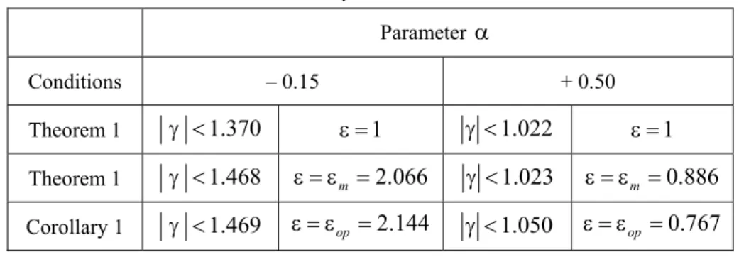
Table 1

Stability Conditions.

Parameter α

Conditions – 0.15 + 0.50

Theorem 1 γ <1.370 ε =1 γ <1.022 ε =1

Theorem 1 γ <1.468 ε = ε =_m 2.066 γ <1.023 ε = ε =_m 0.886

Corollary 1 γ <1.469 ε = ε =_op 2.144 γ <1.050 ε = ε =_op 0.767

5 Conclusion

In this paper we have established a new Lyapunov-Krasovskii method for linear discrete time systems with multiple time delay. Based on this method, two sufficient conditions for delay-independent asymptotic stability of the linear time systems with multiple delays are derived. These conditions stabilities have been expressed in the shape of Lyapunov inequality. Numerical examples are presented to demonstrate the applicability of the present approach.

6 References

[1] S.I. Niculescu, C.E. de Souza, L. Dugard, J.M. Dion: Robust Exponential Stability of

Uncertain Linear Systems with Time-varying Delays, IEEE Transaction on Automatic Control, Vol. 43, No. 5, May 1998, pp. 743 – 748.

[2] L. Dugard, E.I. Verriest: Stability and Control of Time-delay Systems, Springer Berlin/Hei-delberg, 1998.

[3] J.K. Hale, S.M.V. Lunel: Introduction to Functional Differential Equations,

Springer-Verlag, New York, 1993.

[4] V.B. Kolmanovskii, V.R. Nosov: Stability of Functional Differential Equations, Academic Press, Orlando, Florida, 1986.

[5] J.H. Su: Further Results on the Robust Stability of Linear Systems with a Single Delay, Systems and Control Letters, Vol. 23, No. 5, Nov. 1994, pp. 375 – 379.

[6] S.I. Niculescu, C.E. de Souza, J.M. Dion, L. Dugard: Robust Stability and Stabilization for Uncertain Linear Systems with State Delay: Single Delay Case (I). IFAC Symposium on Robust Control Design, Rio de Janeiro, Brazil, 1994, pp. 469 – 474.

[7] S. Boyd, L. El Ghaoui, E. Feron, V. Balakrishnan: Linear matrix inequalities in system and control theory, SIAM Studies in Applied Mathematics, Philadelphia, USA, 1994.

[8] J.H. Su: The Asymptotic Stability of Linear Autonomous Systems with Commensurate

[9] V. Kolmanovskii, J.P. Richard: Stability of Some Linear Systems with Delays, IEEE Transactions on Automatic Control, Vol. 44, No. 5, May 1999, pp. 984 – 989.

[10] M. Malek-Zavarei, M. Jamshidi: Time-delay Systems, Analysis, Optimization and

Applications, Elsevier Science Inc., New York , USA, 1987.

[11] P. Park: A Delay-dependent Stability Criterion for Systems with Uncertain Time-invariant Delays, IEEE Transactions on Automatic Control, Vol. 44, No. 4, Apr. 1999, pp. 876 – 877.

[12] S.I. Niculescu: On Delay-dependent Stability under M odel Transformations of Some

Neutral Linear Systems, International Journal of Control, Vol. 74, No. 6, Apr. 2001, pp. 609 – 617.

[13] J. Chen, G. Gu, C.N. Nett: A New Method for Computing Delay Margins for Stability of

Linear Delay Systems, 33rd IEEE Conference on Decision and Control, Lake Buena Vista, Florida, USA, Vol. 1, Dec. 1994, pp. 433 – 437.

[14] P. Park, Y.S. Moon, W.H. Kwon: A Delay-dependent Robust Stability Criterion for

Uncertain Time-delay Systems, American control conference, Philadelphia, Pennsylvania, June 1998, pp. 1963 – 1964.

[15] E. Fridman, U. Shaked: A Descriptor System Approach to H∞ Control of Linear

Time-delay Systems, IEEE Transactions on Automatic Control, Vol. 47, No. 2, Feb. 2002, pp. 253 – 270.

[16] E. Fridman, U. Shaked: An LMI Approach to Stability of Discrete Delay Systems,

European Control Conference, Cambridge, United Kingdom, Sept. 2003.

[17] E. Fridman, U. Shaked: Delay-dependent H∞ Control of Uncertain Discrete Delay Systems, European Journal of Control, Vol. 11, No.1, 2005, pp. 29 – 37.

[18] E. Fridman, U. Shaked: Stability and Guaranteed Cost Control of Uncertain Discrete Delay Systems, International Journal of Control, Vol. 78, No. 4, March 2005, pp. 235 – 246. [19] V. Kapila, W.M. Haddad: Memoryless H∞ Controllers for Discrete-time Systems with Time

Delay, Automatica, Vol. 34, No. 9, Sept. 1998, pp. 1141 – 1144.

[20] Y.S. Lee, W.H. Kwon: Delay-dependent Robust Stabilization of Uncertain Discrete-time

State-delayed Systems, 15th Triennial World Congress, Barcelona, Spain, 2002.

[21] M.S. Mahmoud: Robust H∞ Control of Discrete Systems with Uncertain Parameters and

Unknown Delays, Automatica, Vol. 36, No. 4, April 2000, pp. 627 – 635.

[22] M.S. Mahmoud: Linear Parameter-varying Discrete Time-delay Systems: Stability and

l2-gain Controllers, International Journal of Control, Vol. 73, No. 6, April 2000, pp. 481 – 494. [23] C.D. Meyer: Matrix analysis and applied linear algebra, SIAM, Philadelphia, 2001.

[24] A.R. Amir-Moez: Extreme Properties of Eigenvalues of a Hermitian Transformations and

Singular Values of Sum and Product of Linear Transformations, Duke Mathematical Journal, Vol. 23, No. 3, Sept. 1956, pp. 463 – 476.

[25] S.B. Stojanovic, D.Lj. Debeljkovic, I. Mladenovic: Simple Exponential Stability Criteria of Linear Discrete Time Delay Systems, Serbian Journal of Electrical Engineering, Vol. 5, No. 2, Nov. 2008, pp. 191 – 198.

[26] S.B. Stojanovic, D.Lj. Debeljkovic, I. Mladenovic: A Lyapunov-Krasovskii Methodology