www.atmos-chem-phys.net/16/15741/2016/ doi:10.5194/acp-16-15741-2016
© Author(s) 2016. CC Attribution 3.0 License.
Model sensitivity studies of the decrease in atmospheric
carbon tetrachloride
Martyn P. Chipperfield1,2, Qing Liang3,4, Matthew Rigby5, Ryan Hossaini6, Stephen A. Montzka7, Sandip Dhomse1, Wuhu Feng1,8, Ronald G. Prinn9, Ray F. Weiss10, Christina M. Harth10, Peter K. Salameh10, Jens Mühle10,
Simon O’Doherty5, Dickon Young5, Peter G. Simmonds5, Paul B. Krummel11, Paul J. Fraser11, L. Paul Steele11, James D. Happell12, Robert C. Rhew13, James Butler7, Shari A. Yvon-Lewis14, Bradley Hall7, David Nance7, Fred Moore7, Ben R. Miller7, James W. Elkins7, Jeremy J. Harrison15,16, Chris D. Boone17, Elliot L. Atlas18, and Emmanuel Mahieu19
1School of Earth and Environment, University of Leeds, Leeds, LS2 9JT, UK 2National Centre for Earth Observation, University of Leeds, Leeds, LS2 9JT, UK
3NASA Goddard Space Flight Center, Atmospheric Chemistry and Dynamics, Greenbelt, Maryland 20771, USA 4Universities Space Research Association, GESTAR, Columbia, Maryland 21046, USA
5Atmospheric Chemistry Research Group, School of Chemistry, University of Bristol, Bristol, BS8 1TS, UK 6Lancaster Environment Centre, Lancaster University, Lancaster, LA1 4YQ, UK
7Global Monitoring Division, NOAA Earth System Research Laboratory, Boulder, Colorado 80305, USA 8National Centre for Atmospheric Science, University of Leeds, Leeds, LS2 9JT, UK
9Massachusetts Institute of Technology, Cambridge, Massachusetts 02139 USA
10Scripps Institution of Oceanography, University of California San Diego, La Jolla, California 92093-0244, USA 11CSIRO Oceans and Atmosphere, Aspendale, Victoria 3195, Australia
12Department of Ocean Sciences, University of Miami, Florida 33149, USA
13Departmet of Geography, University of California, Berkeley, California 94720-4740, USA 14Department of Oceanography, Texas A&M University, College Station, Texas 77840, USA 15Department of Physics and Astronomy, University of Leicester, Leicester, LE1 7RH, UK 16National Centre for Earth Observation, University of Leicester, Leicester, LE1 7RH, UK 17Department of Chemistry, University of Waterloo, Ontario, N2L 3G1, Canada
18Department of Atmospheric Sciences, University of Miami, Miami, Florida 33149, USA 19Institute of Astrophysics and Geophysics, University of Liège, Liège 4000, Belgium
Correspondence to:Martyn P. Chipperfield ([email protected])
Received: 9 July 2016 – Published in Atmos. Chem. Phys. Discuss.: 18 August 2016
Revised: 24 November 2016 – Accepted: 28 November 2016 – Published: 20 December 2016
Abstract.Carbon tetrachloride (CCl4) is an ozone-depleting
substance, which is controlled by the Montreal Protocol and for which the atmospheric abundance is decreasing. How-ever, the current observed rate of this decrease is known to be slower than expected based on reported CCl4 emissions
and its estimated overall atmospheric lifetime. Here we use a three-dimensional (3-D) chemical transport model to inves-tigate the impact on its predicted decay of uncertainties in the rates at which CCl4is removed from the atmosphere by
photolysis, by ocean uptake and by degradation in soils. The
largest sink is atmospheric photolysis (74 % of total), but a reported 10 % uncertainty in its combined photolysis cross section and quantum yield has only a modest impact on the modelled rate of CCl4decay. This is partly due to the limiting
effect of the rate of transport of CCl4from the main
the model shows that uncertainty in ocean loss (17 % of total) has the largest impact on modelled CCl4decay due to its
size-able contribution to CCl4loss and large lifetime uncertainty
range (147 to 241 years). With an assumed CCl4 emission
rate of 39 Gg year−1, the reference simulation with the best estimate of loss processes still underestimates the observed CCl4(overestimates the decay) over the past 2 decades but
to a smaller extent than previous studies. Changes to the rate of CCl4loss processes, in line with known uncertainties,
could bring the model into agreement with in situ surface and remote-sensing measurements, as could an increase in emis-sions to around 47 Gg year−1. Further progress in
constrain-ing the CCl4 budget is partly limited by systematic biases
between observational datasets. For example, surface obser-vations from the National Oceanic and Atmospheric Admin-istration (NOAA) network are larger than from the Advanced Global Atmospheric Gases Experiment (AGAGE) network but have shown a steeper decreasing trend over the past 2 decades. These differences imply a difference in emissions which is significant relative to uncertainties in the magni-tudes of the CCl4sinks.
1 Introduction
Carbon tetrachloride (CCl4)is an important ozone-depleting
substance (ODS) and greenhouse gas (GHG) (WMO, 2014). Because of its high ozone depletion potential (ODP), it has been controlled since the 1990 London Amendment to the 1987 Montreal Protocol. Historically CCl4 was used as a
solvent, as a fire-retarding chemical and as a feedstock for production of chlorofluorocarbons (CFCs) and their replace-ments, though current production should be limited to feed-stock, process agents and other essential applications (WMO, 2014).
In response to the controls of dispersive uses under the Montreal Protocol and its adjustments and amendments, the atmospheric burden of CCl4 peaked at around 106 ppt
(pmol mol−1) in 1990 and then declined at about 1 ppt year−1
(around 1 % year−1) through 2005 with indications of a faster
rate of decline, around 1.3 ppt year−1, since then. Carpenter
et al. (2014) give the recent rate of decline (2011–2012) as 1.1–1.4 ppt year−1, depending on the observation network.
However, despite this ongoing decline in atmospheric CCl4
burden there is a significant discrepancy in the known CCl4
budget. The atmospheric decline is significantly slower than would be expected based on reported production to disper-sive and non-disperdisper-sive uses, and current estimates of the strength of CCl4sinks.
The main removal process for atmospheric CCl4 is slow
transport to the stratosphere followed by photolysis at UV wavelengths (see Burkholder et al., 2013). This photoly-sis mainly occurs in the middle stratosphere, and so the rate of removal depends also on the slow transport of CCl4
through the stratosphere by the Brewer–Dobson circulation, for which the speed can vary. The other significant sinks for CCl4are ocean uptake (Krysell et al., 1994) and degradation
in soils (Happell and Roche, 2003; Happell et al., 2014). Uncertainties in the CCl4 budget, where emissions
de-rived from reported production magnitudes underestimate the sources needed to be consistent with our understanding of CCl4loss processes and its change in atmospheric
abdance, have been an issue for almost 2 decades. These un-certainties have been highlighted in many of the 4-yearly World Meteorological Organization (WMO)/United Nations Environmental Programme (UNEP) ozone assessments, in-cluding the most recent one in 2014. WMO (2014) stated that estimated sources and sinks of CCl4 remain
inconsis-tent with observations of its abundance. The report used an overall atmospheric CCl4lifetime of 26 years to infer a need
for 57 (40–74) Gg year−1emissions of CCl
4, which greatly
exceeded that expected based on reported production for dis-persive uses.
Liang et al. (2014) used a three-dimensional (3-D) chemistry–climate model (CCM) to investigate possible causes for this “budget gap” in CCl4. They performed a series
of experiments with different assumptions of CCl4emissions
and overall atmospheric lifetime. In particular they used the observed interhemispheric gradient (IHG) of CCl4 to infer
the magnitude of ongoing emissions missing in the current inventories, with some information on their distribution be-tween the hemispheres. They inferred that the mean global emissions of CCl4were 39 (34–45) Gg year−1and the
corre-sponding overall CCl4lifetime was 35 (32–37) years. In
con-trast their model calculated an overall atmospheric lifetime of CCl4of 25.8 years, based on a calculated partial lifetime for
photolysis loss of 47 years and specified partial lifetimes for ocean and soil loss of 79 and 201 years, respectively.
The partial lifetime of CCl4due to loss by photolysis was
calculated in the recent Stratospheric Processes And their Role in Climate (SPARC) lifetimes report (SPARC, 2013; Chipperfield et al., 2013) using six chemistry–climate mod-els. The modelled steady-state CCl4partial lifetime for
year-2000 conditions varied from 41.4 to 54.3 years with a mean of 49.9 years. The large spread in model values was attributed to different circulation rates in the models; generally a faster tropical upwelling circulation gave rise to a shorter lifetime. To obtain an overall recommended photolysis lifetime value of 44 years, SPARC (2013) combined those model results with a shorter lifetime of 40 years based on stratospheric tracer–tracer correlations and the loss of CCl4 relative to
CFC-11 (CFCl3).
Since the publication of Liang et al. (2014) there has been renewed interest in the CCl4 budget gap. Rhew and
Happell (2016) re-evaluated the global CCl4soil sink using
new observations and an improved land cover classification scheme. They derived the partial lifetime of CCl4with
the ocean sink to be 183 (147–241) years. Note that this esti-mate of the ocean sink is different to the earlier value of 210 (157–313) years provided by the same authors for the recent SPARC report on carbon tetrachloride (SPARC, 2016) prior to their most recent analysis. These partial lifetimes for the soil and ocean sink are both much longer than previous es-timates used in Liang et al. (2014), as recommended in Car-penter et al. (2014). The recent papers also provide a revised uncertainty range which can be used to constrain model–data comparisons.
The aim of this paper is to quantify the magnitude of CCl4
emissions over the recent past using the most up-to-date in-formation on the main CCl4loss processes using the
frame-work of a particular 3-D model. In particular, we use the es-timated uncertainties in the CCl4 loss processes to further
constrain the likely range of emissions. We also test the re-sults of Liang et al. (2014) using a different model of atmo-spheric chemistry and transport which we compare to a range of available observations, thereby contributing to more ro-bust conclusions. Section 2 describes the CCl4observations
that we use and our 3-D chemical transport model (CTM). Section 3 compares our model simulations with these obser-vations and quantifies the emissions required for model–data agreement. Section 3 also discusses our results in the con-text of other recent work. Our conclusions are presented in Sect. 4.
2 CCl4observations and 3-D model
2.1 NOAA and AGAGE CCl4
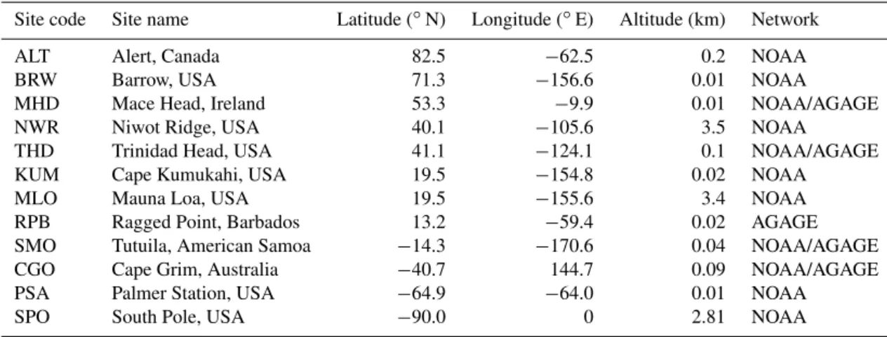
We have used surface CCl4observations from 11 National
Oceanic and Atmospheric Administration/Earth System Re-search Laboratory (NOAA/ESRL) cooperative global air sampling sites (Hall et al., 2011) and 5 sites from the Ad-vanced Global Atmospheric Gases Experiment (AGAGE) network (Simmonds et al., 1998; Prinn et al., 2000, 2016; http://agage.mit.edu/) over 1995–2015 (Table 1). NOAA ob-servations consist of paired air samples collected in flasks ap-proximately weekly and sent to Boulder, Colorado, for anal-ysis by gas chromatography with electron capture detection (GC-ECD), and they are reported on the NOAA-2008 scale. NOAA global and hemispheric averages are computed by weighting station data by cosine of latitude. Actual NOAA station latitudes are used, except for South Pole, for which we use 70.5◦S. AGAGE observations are made at a 40 min frequency using GC-ECD instruments located at remote sites and are reported on the Scripps Institution of Oceanography 2005 scale (SIO-05). AGAGE data were filtered to remove above-baseline “pollution” events using the method outlined in O’Doherty et al. (2001), and the remaining baseline mole fractions were averaged each month. AGAGE hemispheric and global averages were calculated using the AGAGE 12-box model and the method described in Rigby et al. (2014).
Briefly, semi-hemispheric monthly-mean AGAGE baseline data were used to constrain emissions with the model. Global average mole fractions were extracted from the a posteriori forward model run.
2.2 ACE
The Atmospheric Chemistry Experiment–Fourier transform spectrometer (ACE-FTS) is on the SCISAT satellite, which was launched in early 2004. ACE-FTS uses the sun as a light source to record limb transmission through the Earth’s atmo-sphere (∼300 km effective length) during sunrise and sun-set (“solar occultation”). ACE-FTS covers the spectral re-gion 750 to 4400 cm−1 with a resolution of 0.02 cm−1 and
can measure vertical profiles for more trace species than any other satellite instrument, although it only records spectra for, at most, 30 occultation events per day (Bernath, 2017). Carbon tetrachloride is one of the species routinely avail-able in the latest v3.5 processing; however the retrieved pro-files are biased high by up to∼20–30 % (Allen et al., 2009;
Brown et al., 2011; Harrison et al., 2016).
Recently, an improved ACE-FTS CCl4retrieval has been
devised (Harrison et al., 2016), and this will form the basis for the upcoming processing version 4.0 of ACE-FTS data. This preliminary retrieval, which is used here, is available for 527 occultations measured during March and April 2005. The improvements include (a) new high-resolution infrared absorption cross sections for air-broadened carbon tetrachlo-ride; (b) a new set of microwindows which avoid spectral re-gions where the line parameters of interfering species do not adequately calculate the measured ACE-FTS spectra; (c) the addition of new interfering species missing from v3.5, e.g. peroxyacetyl nitrate (PAN); and (d) an improved instrumen-tal lineshape designed for the upcoming v4.0 processing.
2.3 NDACC column CCl4observations
Carbon tetrachloride can also be retrieved from high-resolution infrared solar spectra recorded at ground-based stations. A total column time series spanning the 1999– 2015 period, updated to be consistent with Rinsland et al. (2012), is available from the Jungfraujoch station (Swiss Alps, 46.5◦N, 8◦E, 3580 m a.s.l.) and will be used here, but an effort is ongoing to retrieve CCl4 from other NDACC
sites (Network for the Detection of Atmospheric Composi-tion Change; see http://www.ndacc.org).
Rinsland et al. (2012) provide a thorough description of the approach which allows the retrieval of CCl4total columns
from ground-based FTIR (Fourier transform infrared) so-lar absorption spectra. Briefly, the strong CCl4 ν3 band at
794 cm−1 is used, and a broad window spanning the 785– 807 cm−1 spectral range is fitted, accounting for main
in-terferences by H2O, CO2 and O3, as well as by a dozen
Table 1.List of NOAA and AGAGE stations which provided CCl4observations.
Site code Site name Latitude (◦N) Longitude (◦E) Altitude (km) Network
ALT Alert, Canada 82.5 −62.5 0.2 NOAA
BRW Barrow, USA 71.3 −156.6 0.01 NOAA
MHD Mace Head, Ireland 53.3 −9.9 0.01 NOAA/AGAGE
NWR Niwot Ridge, USA 40.1 −105.6 3.5 NOAA
THD Trinidad Head, USA 41.1 −124.1 0.1 NOAA/AGAGE
KUM Cape Kumukahi, USA 19.5 −154.8 0.02 NOAA
MLO Mauna Loa, USA 19.5 −155.6 3.4 NOAA
RPB Ragged Point, Barbados 13.2 −59.4 0.02 AGAGE
SMO Tutuila, American Samoa −14.3 −170.6 0.04 NOAA/AGAGE
CGO Cape Grim, Australia −40.7 144.7 0.09 NOAA/AGAGE
PSA Palmer Station, USA −64.9 −64.0 0.01 NOAA
SPO South Pole, USA −90.0 0 2.81 NOAA
at 791 cm−1have to be accounted for and properly modelled
by the retrieval algorithm when dealing with such a wide-window approach. The associated error budget indicates to-tal random and systematic uncertainties on individual toto-tal column measurements of less than 7 and 11 %, respectively. 2.4 HIPPO data
In situ measurements of CCl4obtained during the HIAPER
Pole-to-Pole (HIPPO) aircraft mission have also been con-sidered (Wofsy, 2011; Wofsy et al., 2012). HIPPO consisted of a series of five campaigns over the Pacific Basin using the National Science Foundation (NSF) Gulfstream V air-craft: HIPPO-1 (January 2009), HIPPO-2 (November 2009), HIPPO-3 (March/April 2010), HIPPO-4 (June 2011) and HIPPO-5 (August/September 2011). Across the campaigns, sampling spanned a large latitude range, extending from near the North Pole to coastal Antarctica, and from the surface to∼14 km. Measured CCl4mixing ratios were derived from
analysis of whole-air samples using GC-MS (mass spectrom-etry) by both NOAA/ESRL and the University of Miami from both pressurised glass and stainless-steel flasks. Results from both laboratories were provided on a scale consistent with NOAA/ESRL.
2.5 TOMCAT 3-D chemical transport model
We have used the TOMCAT global atmospheric 3-D off-line CTM (Chipperfield, 2006) to model atmospheric CCl4. The
TOMCAT simulations were forced by winds and tempera-tures from the 6-hourly European Centre for Medium-Range Weather Forecasts (ECMWF) ERA-Interim reanalyses (Dee et al., 2011). The simulations covered the period 1996 to 2016 with a horizontal resolution of 2.8◦×2.8◦and 60
lev-els from the surface to ∼60 km. The model contained 11
parameterised CCl4 tracers that evolved in response to
sur-face emissions and loss by calculated atmospheric photolysis rates and specified partial lifetimes with respect to uptake by oceans or soils (see Table 2). Different tracers (CTC1–CTC8)
use different specified combinations of the emission and loss processes described below. Tracer CTC1 is the reference tracer with the current best estimate values of the loss pro-cesses. The annually varying global emissions were derived with the global one-box model used in recent WMO ozone assessments (for details, see Velders and Daniel, 2014), as-suming a 35-year total lifetime for CCl4, and the long-term
surface observations of CCl4from the NOAA Global
Mon-itoring Division (GMD) network (Hall et al., 2011). These emissions were distributed spatially according to Xiao et al. (2010).
For the photolysis sink, monthly-mean photolysis rates were calculated using a stand-alone version of the TOM-CAT/SLIMCAT stratospheric chemistry scheme and kinetic data from Sander et al. (2011). Hourly model output was av-eraged to produce monthly-mean photolysis rates as a func-tion of latitude and altitude. To assess the model sensitiv-ity to the photolytic loss, two model tracers used these rates changed by±10 %, in line with the recommended combined uncertainty in cross sections and quantum yields from Sander et al. (2011). In reality this will be a lower limit of uncer-tainty in the modelled photolysis rates because it does not account for errors in the model radiative transfer code, ozone distribution etc. This is difficult to quantify absolutely, but we would note that the TOMCAT/SLIMCAT photolysis scheme has performed well in intercomparisons of radiative transfer codes (e.g. SPARC CCMVal, 2010; Sukhodolov et al., 2016). For comparisons using a prescribed ozone profile and solar fluxes, SPARC CCMVal (2010) found excellent agreement between models for the calculation of photolysis rates for N2O and CFC-11, which are species with similar photolysis
sinks to CCl4. Therefore, we would suggest that the largest
uncertainty in the modelled CCl4photolysis rate does indeed
Table 2.Summary of the TOMCAT 3-D CTM simulated CCl4tracers.
Tracer Emissions Atmospheric loss Surface loss Overall
(Gg year−1)b photolysis partial lifetimes lifetime
(years) (years)a
Photochemical Partial Ocean Soil
data lifetimea
CTC1 39.35 JPL 41.9 183 375 31.9
CTC1s 39.35 JPL 41.9 210 375 31.9
CTC2 39.35 JPL 41.8 147 375 30.4
CTC2s 39.35 JPL 41.8 157 375 30.4
CTC3 39.35 JPL 41.9 241 375 33.7
CTC3s 39.35 JPL 41.9 313 375 33.7
CTC4 39.35 JPL 41.9 183 288 31.5
CTC5 39.35 JPL 41.9 183 536 32.4
CTC6 39.35 0.9×JPL 43.5 183 375 32.9
CTC7 39.35 1.1×JPL 40.4 183 375 31.1
CTC8 45.25 JPL 41.9 183 375 32.0
aOverall and photolysis partial lifetimes for each tracer calculated from model burden and loss rates.bMean of
interannually varying emissions from 1996 to 2015 (see Fig. 1).
The ocean sink was represented by specifying a partial lifetime of CCl4 with respect to removal from the surface
grid boxes over the oceans. We used the recent results of But-ler et al. (2016), who derived this partial lifetime to be 183 (147–241) years. (We also performed a simulation with the values presented in SPARC (2016) of 209 (157–313) years for tracers CTC1s, CTC2s and CTC3s). For the partial life-time of CCl4 loss over soil we used the recently published
values of Rhew and Happell (2016), i.e. a best estimate of 375 years and an uncertainty range of 288–536 years. Both the ocean and soil sinks were assumed to be constant in time and were treated to be spatially uniform over ocean and land grid boxes, respectively, following the method of Liang et al. (2014).
The TOMCAT run was spun up for 4 years, and then all tracers were scaled to match “observed” global mean CCl4
values in early 1996 (based on WMO/UNEP A1 scenario values, derived from an average of AGAGE and NOAA sur-face measurements). The model was then run for a further 20 years until 2016.
3 Results 3.1 Emissions
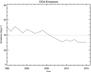
Figure 1 shows the evolution of the prescribed surface emis-sions in the model run (i.e. for tracers CTC1–CTC7) over 1995–2015. As noted in Sect. 2.5, these were derived from atmospheric observations and a global box model assum-ing a constant overall CCl4 lifetime of 35 years. For the
purposes of this study, these prescribed emissions simply provide a time-dependent reference input dataset for the
3-Figure 1.Time variation of global annual emissions (Gg year−1) derived from measured global atmospheric changes and a global box model (solid line). The emission record was used for the stan-dard TOMCAT model experiments. The mean emissions over the period 1996–2015 are 39.35 Gg year−1(indicated by dotted line).
D model. Comparisons of the 3-D model with atmospheric observations can then provide further, more detailed infor-mation on the likely CCl4 lifetime and the emissions
re-quired to match the atmospheric observations. Note the in-ferred lifetime and emissions are model-dependent. Figure 1 shows that the prescribed emissions decrease from around 45 to about 35 Gg year−1 with a more rapid decrease
3.2 Comparison with observations
First we compare the simulated CCl4tracers with
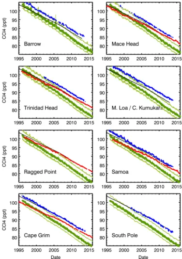
observa-tions to evaluate the performance of the basic model. Figure 2 compares model results (in green) with surface observations at eight sites from the NOAA (blue line) and AGAGE (red line) networks for which CCl4data are available. Sites where
measurements are reported by both networks – i.e. Mace Head, Trinidad Head, Samoa and Cape Grim – show that NOAA observations are larger than AGAGE by about 5 ppt in 1996, which decreases to about 1 ppt by 2014. The panels also show global mean CCl4values from the WMO (2014)
A1 scenario (black line), which was constructed by a sim-ple average of the global means derived with AGAGE and NOAA data, and therefore typically lies between the re-sults from the two networks at these sites. Note that the TOMCAT runs were scaled globally to agree with the 2014 WMO/UNEP baseline scenario in 1996, which was derived from an average of results from the two networks. Figure 2 shows that CCl4from the TOMCAT reference tracer CTC1
decays more rapidly than observed in the networks. By 2013 tracer CTC1 underestimates the WMO/UNEP scenario by about 8 ppt. Note that although we are using an updated emis-sion dataset, which is derived from observations, the level of agreement also depends on the overall CCl4lifetime
speci-fied or calculated in each model.
Figure 3 compares total column CCl4 from model run
CTC1 with FTIR observations at Jungfraujoch. At present this is the only ground-based station with a long-term dataset for column CCl4. Although the geographical coverage is
therefore limited, the comparison does allow us to test the modelled CCl4 through the depth of the troposphere and
not just at the surface (as in Fig. 2). An initial compari-son between the observed and modelled columns indicated a bias of about 15 %, with TOMCAT lying below the FTIR data. Since the latter could be affected by a systematic un-certainty of up to 10–11 % (see Table 1 in Rinsland et al., 2012), we allowed for a×0.9 scaling of the column amounts. Figure 3 shows the model still tends to underestimate the scaled FTIR column by about 0.05×10¹⁵molecules cm−2
(about 5 %). This difference is similar to that between the NOAA and AGAGE observed surface mixing ratios in the 1990s and early 2000s, so this limits the extent to which we can assess the consistency of the surface and column observations. Despite any disagreements in the absolute amount of observed CCl4, the relative decay rates can still
be compared. The FTIR column observations show a de-cline of 1.3×10¹³molecules cm−2year−1 (1.18 % year−1),
which compares fairly well with the modelled value (control tracer CTC1) of 1.5×10¹³molecules cm−2year−1
(1.36 % year−1). Therefore, it appears that the model slightly overestimates the observed relative decay of column CCl4as
well as the relative decline rate measured at the surface (1.1– 1.2 % year−1from 1996 to 2013).
Figure 2. Comparison of modelled surface CCl4 concentration
(ppt) with observations at eight stations in the AGAGE (red line) or NOAA (blue line) networks. Also shown is the CCl4global mean
surface mixing ratio from WMO (2014) scenario A1 (black line). The dark green line shows model control tracer CTC1, and light green lines show this tracer CTC1 line displaced by+3 and−2 ppt to aid comparisons with the slope of the NOAA and AGAGE ob-servations. This range is arbitrary but indicates how the model line would be displaced if the CTC1 tracer had been initialised to agree with either the NOAA or AGAGE global mean CCl4abundance in
1996.
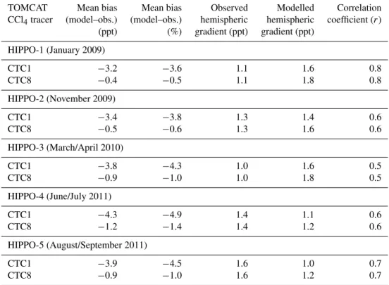
The HIPPO campaigns provided flask sampling of air at a wide range of latitudes from the surface to about 14 km. Fig-ure 4 shows a comparison of the results from the analysis of flasks collected during HIPPO from the surface to 1.5 km al-titude from five campaigns from January 2009 until Septem-ber 2011. Also shown are results from model tracers CTC1 (control) and CTC8 (increased emissions), along with the monthly-mean observations from NOAA and AGAGE sur-face stations. Comparisons between the model and HIPPO observations are summarised in Table 3. Consistent with the results from the surface network, the HIPPO results show larger CCl4mixing ratios in the Northern Hemisphere
Table 3. Summary of model–measurement comparisons for boundary layer (surface–1.5 km) CCl4 observations during HIPPO aircraft
missions.
TOMCAT Mean bias Mean bias Observed Modelled Correlation
CCl4tracer (model–obs.) (model–obs.) hemispheric hemispheric coefficient (r)
(ppt) (%) gradient (ppt) gradient (ppt)
HIPPO-1 (January 2009)
CTC1 −3.2 −3.6 1.1 1.6 0.8
CTC8 −0.4 −0.5 1.1 1.8 0.8
HIPPO-2 (November 2009)
CTC1 −3.4 −3.8 1.3 1.4 0.6
CTC8 −0.5 −0.6 1.3 1.6 0.6
HIPPO-3 (March/April 2010)
CTC1 −3.8 −4.3 1.0 1.6 0.5
CTC8 −0.9 −1.0 1.0 1.8 0.5
HIPPO-4 (June/July 2011)
CTC1 −4.3 −4.9 1.4 1.1 0.6
CTC8 −1.2 −1.4 1.4 1.2 0.6
HIPPO-5 (August/September 2011)
CTC1 −3.9 −4.5 1.6 1.0 0.7
CTC8 −0.9 −1.0 1.6 1.2 0.7
Figure 3. Time series of total column CCl4
(×1015molecules cm−2) at the Jungfraujoch NDACC
sta-tion, Switzerland (46.5◦N, 8◦E) (blue line). The observations have been scaled by 0.9 to account for a possible high bias in the CCl4
retrieved columns (see Sect. 3.2). Also shown are results from model control tracer CTC1 (green line). The straight lines are the linear fits to the observations and model output.
in the HIPPO observations, but this is larger in HIPPO-3 (March/April 2010), for example, than in HIPPO-1 (Jan-uary 2009). The HIPPO campaigns occurred when the differ-ence between the surface NOAA and AGAGE observations had decreased but is still apparent (Figs. 2 and 4). It appears that the NOAA observations, which are larger than AGAGE,
are in better agreement with the HIPPO data at locations where both surface networks sampled (±1◦of latitude), but note that the HIPPO data are reported on the NOAA cal-ibration scale. For example, across all of the HIPPO cam-paigns, the mean bias (NOAA minus HIPPO) is<0.1,−0.1 and 0.2 ppt at MHD, SMO and CGO, respectively. Similarly, for AGAGE at these sites, the mean bias is−1.7,−1.6 and
−1.4 ppt, respectively. For the near-surface values plotted in Fig. 4, the model qualitatively captures the interhemispheric gradient (see Sect. 3.3 for more discussion). Tracer CTC1 underestimates the HIPPO observations, with a mean cam-paign bias in the range of−3.6 to −4.9 % (Table 3). The agreement is improved by assuming additional emissions in tracer CTC8 (see also Fig. 2), which has a smaller mean bias in the range of−0.5 to−1.4 %.
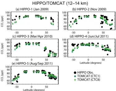
Figure 5 shows HIPPO–TOMCAT comparisons in the up-per troposphere–lower stratosphere (UTLS) at 12–14 km. The model captures the latitudinal gradient in the obser-vations, including the large decreases at high latitudes in stratospheric air. This high-latitude agreement is worst in the northern polar region in November 2009 and the southern po-lar region in June/July 2011, when the comparisons are likely to be affected by structure in the tracer fields caused by large gradients around the polar vortex. Nevertheless, Fig. 5 shows that the model performs realistically in terms of transport of CCl4to higher altitudes and through the lower stratosphere
(a) HIPPO-1 (Jan 2009)
-50 0 50
80 85 90 95 CCl 4 (ppt)
HIPPO/TOMCAT (0–1.5 km)
(b) HIPPO-2 (Nov 2009)
-50 0 50
80 85 90 95
(c) HIPPO-3 (Mar/Apr 2010)
-50 0 50
80 85 90 95 CCl 4 (ppt)
(d) HIPPO-4 (Jun/Jul 2011)
-50 0 50
Latitude (degrees) 80
85 90 95
(e) HIPPO-5 (Aug/Sep 2011)
-50 0 50
Latitude (degrees) 80 85 90 95 CCl 4 (ppt) HIPPO Obs. NOAA Obs. AGAGE Obs. TOMCAT (CTC1) TOMCAT (CTC8)
Figure 4. Latitude cross section of HIPPO observations of CCl4
(ppt, black circles) between the surface and 1.5 km altitude from flights during five campaigns between January 2009 and Septem-ber 2011. Also shown are mean surface observations from the AGAGE (red diamond) and NOAA (blue+) networks (see Table 1 and Fig. 2) for the months of the campaign. Results from model tracers CTC1 and CTC8 are also shown.
Comparison with CCl4profiles in the stratosphere allows
us to test how well the model simulates the photolysis sink. Figure 6 compares mean modelled profiles of CCl4with the
recent ACE-FTS research retrievals (Harrison et al., 2016) from March to April 2005 in three latitude bands. The fig-ure shows results from the control tracer CTC1 along with the tracers CTC6 and CTC7, which have±10 % change in photolysis rate. Overall the model reproduces the observed decay of CCl4in the stratosphere well, which confirms that
the stratospheric photolysis sink and transport are well mod-elled in TOMCAT, with a reasonable corresponding lifetime. However, the difference between tracer CTC1 and tracers CTC6/CTC7 is not large compared to the model–ACE dif-ferences. Hence, while the available ACE data can confirm the basic realistic behaviour of the model in the stratosphere, they are not able to evaluate the model more critically. When available over the duration of the ACE mission, the full v4 retrieval will allow more comprehensive and critical com-parisons over a wider range of latitudes and seasons. Also, Fig. 6 illustrates the need to compare the model transport separately through comparison of other tracers with differ-ent lifetimes and distributions, before factoring the effect of photolytic loss of CCl4.
3.3 Impact of uncertainties in sinks
Figure 7 shows the partial CCl4 photolysis lifetime
diag-nosed from reference tracer CTC1. There is large short-term (monthly) variability in the instantaneous lifetime. Even for the annual mean lifetime there is significant interannual
vari-(a) HIPPO-1 (Jan 2009)
-50 0 50
50 60 70 80 90 100 CCl 4 (ppt)
HIPPO/TOMCAT (12–14 km)
(b) HIPPO-2 (Nov 2009)
-50 0 50
50 60 70 80 90 100
(c) HIPPO-3 (Mar/Apr 2010)
-50 0 50
50 60 70 80 90 100 CCl 4 (ppt)
(d) HIPPO-4 (Jun/Jul 2011)
-50 0 50
Latitude (degrees) 50 60 70 80 90 100
(e) HIPPO-5 (Aug/Sep 2011)
-50 0 50
Latitude (degrees) 50 60 70 80 90 100 CCl 4
(ppt) HIPPO Obs.TOMCAT (CTC1)
TOMCAT (CTC8)
Figure 5.Latitude cross section of HIPPO observations of CCl4 (ppt, black circles) between 12 and 14 km altitude from flights dur-ing five campaigns between January 2009 and September 2011. Re-sults from model tracers CTC1 and CTC8 are also shown.
ability which is driven by interannual meteorological vari-ability. The diagnosed annual mean CCl4lifetime over this
period varies from around 39.5 years in 2010 to around 46 years in 2008. The impact of the meteorological variabil-ity was confirmed by running the model for 4 years with an-nually repeating meteorology from two different years (2008 and 2010). The results of these runs are shown by the+ sym-bols, which show constant annual mean partial lifetimes but with a large (∼7 year) difference. This∼7-year difference in the photolysis partial lifetime would correspond to a∼4-year difference in the overall atmospheric lifetime after combin-ing with current best estimates of the ocean and soil sinks. This difference in overall lifetime will translate into a dif-ference of∼6 Gg year−1in the emissions required to match
the observations. Therefore, this circulation-driven variabil-ity can significantly influence top-down emission estimates and their interannual changes. This also shows the derived mean emission estimates will be model- and/or meteorology-dependent, and need to be treated with caution.
30–60 N (n = 92)
0 50 100 150 200
CCl4 (ppt)
10 15 20 25 30
Altitude (km)
25–25 N (n = 152)
0 50 100 150 200
CCl4 (ppt)
10 15 20 25 30
30–60 S (n = 74)
0 50 100 150 200
CCl4 (ppt)
10 15 20 25 30
(a) (b) (c)
o o o
Figure 6.Mean profiles of CCl4from March to April 2005 as determined from the recent ACE-FTS research retrievals (Harrison et al.,
2016) (black line) for latitude bands(a)30–60◦N,(b)25◦S–25◦N and(c)30–60◦S. The number of observed profiles which contribute
to the mean is given in the titles (n). The dashed lines show the standard deviation of the observations. Also shown are mean profiles from model control tracer CTC1 for the same latitude bins and time period (green line) and the range of values produced from sensitivity runs CTC6 and CTC7 with±10 % change in CCl4photolysis rate (orange shading, difficult to see). Note that the model profiles are averages over the indicated spatial regions and are not sampled at the exact locations of the ACE-FTS measurements.
CCl4 partial photolysis lifetime
Date
Lifetime (years)
Figure 7.Modelled instantaneous CCl4partial photolysis lifetime
diagnosed from reference tracer CTC1 (dotted line, value every 20 days) and the same curve with 1-year smoothing (green solid line). The ∗symbols indicate the annual mean CCl4 partial
life-time from this tracer. Also shown are annual mean lifelife-time results from 4-year simulations (2008–2011) with repeating winds for 2008 (black+) and 2010 (red+) meteorology.
the younger end of the modelled range, which is consistent with a slightly young stratospheric age of air in this version of the TOMCAT/SLIMCAT model when forced with ERA-Interim reanalyses (Chipperfield, 2006; Monge-Sanz et al., 2007). Table 2 shows that, as expected, changing the
magni-tude of the soil and ocean sink does not affect the calculated photolysis partial lifetime.
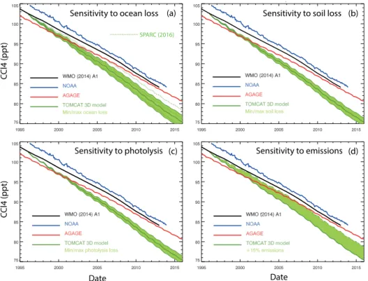
Figure 8a shows the comparison of control model tracer CTC1 vs. global mean surface observations, along with model sensitivity tracers CTC2 and CTC3 with mini-mum/maximum estimates for the ocean sink. This global comparison of tracer CTC1 shows similar behaviour to the individual stations in Fig. 2; the control run slightly overes-timates the observed rate of decay (for the level of emissions assumed). The uncertainty in the ocean sink has a large rel-ative impact on the decay rate of CCl4, relative to the
mis-match with the AGAGE and NOAA datasets. Figure 8a also shows results from tracers CTC1s, CTC2s and CTC3s, which use the best estimate and range of the ocean loss lifetimes from the SPARC (2016) report. The partial lifetime used for CTC1s (210 years) gives a slower decay than tracer CTC1, which uses the latest recommended value (183 years). The uncertainty range between tracers CTC2s and CTC3s is also slightly larger than between CTC2 and CTC3. These trac-ers are included for comparison with the SPARC (2016) re-port, though we reiterate that the values published in Butler et al. (2016) are the latest recommendations for the ocean sink.
Figure 8b is a similar plot which uses model tracers CTC4 and CTC5 to investigate the impact of uncertainty in the soil loss rate. Here the impact on the modelled CCl4decay rate
is relatively small due to the relatively long lifetime of CCl4
with respect to loss by soils.
Figure 8c shows the effect of a±10 % change in pho-tolysis rate on the modelled CCl4 decay using runs CTC6
Sensitivity to ocean loss
Sensitivity to emissions Sensitivity to soil loss
Sensitivity to photolysis (a)
(d) (b)
(c)
Date Date
C
Cl4 (ppt)
C
Cl4 (ppt)
SPARC (2016)
Figure 8.Observed global mean surface CCl4from AGAGE (red) and NOAA (blue) networks, along with merged observational dataset from
WMO (2014) scenario A1 (black line). These are compared with results from TOMCAT model run CTC1 (dark green line) and different sensitivity tracers in each panel with the range given as a light green band:(a)an ocean sink of 147 (tracer CTC2) and 241 (CTC3) years,(b)a soil sink of 288 (CTC4) and 536 (CTC5) years,(c)a±10 % change in stratospheric photolysis (CTC6 and CTC7) and(d)a 15 % increase in emissions (CTC8). Note that in(d)the light green shading only shows an increase relative to control tracer CTC1 as the sensitivity tracer considered had increased emissions. Panel(a)also includes results from TOMCAT tracers which use the SPARC (2016) value for the ocean sink of 183 (CTC1s) years and the uncertainty range of 157 (CTC2s)–313 (CTC3s) years (green dashed lines).
these two runs change by a lot less than 10 % (e.g. 41.9 to 43.5 years; 3.8 % – see Table 2). This is due to compensa-tion in the modelled chemical loss rates in the stratosphere (J[CCl4]). A faster photolysis rateJ will decrease the
con-centration of CCl4, leading to a partial cancellation in the
product. This would be a property of any source gas with a stratospheric sink and large tropospheric reservoir. This par-tial cancellation in the stratospheric loss rate means that un-certainty in the ocean sink still dominates. This is likely to be the case even with a much larger assumed uncertainty in the modelled photolysis rates (e.g.±20 %).
Figure 8d shows the results from tracer CTC8, which as-sumes 15 % larger emissions than tracer CTC1. This increase in emissions (to a mean of around 45 Gg year−1) brings the
model in closer agreement with the rates of decay seen in the surface networks, especially that depicted by the mean of NOAA and AGAGE observations. A 20 % increase in emis-sions (to a mean of around 47 Gg year−1) would give even
better agreement for this setup of the TOMCAT model (not shown). Over the period 1996–2015, the slopes of the lin-ear fits to the lines for tracers CTC1 and CTC8 are −1.36 and−1.20 ppt year−1, respectively. This 0.16 ppt year−1
dif-ference in slope corresponds to a difdif-ference in emissions of
6 Gg year−1 between the two tracers (Table 2). The linear
fits to the global mean NOAA and AGAGE lines in Fig. 8d over the same period are −1.15 and −1.01 ppt year−1,
re-spectively, although it should be noted that the AGAGE vari-ation is not linear over this time frame. Nevertheless, this 0.14 ppt year−1 difference in the mean slope from the two
surface networks (equivalent to∼5 Gg year−1emissions) is
significant when compared to the magnitude of the emis-sions needed to fit the observations under different lifetime assumptions. Therefore, resolving this issue of the absolute difference in the concentrations reported by the two networks will be important for a detailed quantification of the CCl4
budget, and that work is ongoing.
Figure 8 shows that current uncertainty in the CCl4
and our current best estimate of the partial CCl4 lifetimes
would require emissions of around 47 Gg year−1 for
TOM-CAT.
3.4 Interhemispheric gradient
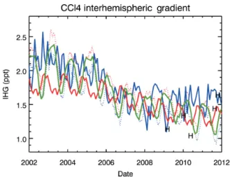
Figure 9 shows the observed interhemispheric gradient (IHG) in CCl4 derived from the NOAA and AGAGE networks
along with results from model tracer CTC1. The observations show that the IHG decreased from about 1.5–2.0 ppt around 2002 to 1.0–1.5 ppt around 2010. Although both networks show this behaviour, the IHG from the NOAA network is per-sistently larger by about 0.3 ppt than from the AGAGE net-work, except for the period 2006–2009, when the IHG values are similar. Throughout the period shown there is not much correspondence between the variations seen in the two obser-vational records as the timing of the seasonal cycles is often different. The NOAA results, which are derived directly from low-frequency (1 per week) station observations, show more variability than the AGAGE results, which are derived from a 12-box model. The modelled IHG also shows a decreasing trend from around 2002 until 2012. However, the modelled IHG shows a regular annual cycle which does not match the observations. In the middle part of the period, when there is a discernible annual cycle in the IHG observed by both networks, the modelled annual cycle is out of phase. We have investigated whether the sparse sampling of the NOAA and AGAGE networks may be responsible for some of the differences between the observations and with the model. Figure 9 shows results of the model tracer CTC1 sampled like the AGAGE and NOAA networks (i.e. at the locations give in Table 1). Compared to using the whole model hemi-spheric grid, sampling at the station locations only changes the IHG slightly; for example the model’s IHG sampled at the AGAGE sites is about 0.3 ppt larger than that sampled at the NOAA sites, which is in the opposite sense to the differences in the observations. However, the modelled annual cycle is still out of phase with the observations in the 2006–2010 pe-riod. Some information on the CCl4IHG is also given by the
comparison with HIPPO data in Fig. 4 and Table 3. Over the course of the campaigns, which sample air over the Pacific, the IHG based on the HIPPO sampling varies from 1.0 ppt in HIPPO-3 to 1.6 ppt in HIPPO-5. This variation reflects sea-sonal variability rather than any long-term trend. Figure 9 shows that the model does not reproduce the timing of this variation.
Overall, Fig. 9 shows that there are still details in the CCl4
IHG that merit further investigation. There are limitations of the TOMCAT model setup used in this study. The assumed emission distribution (from Xiao et al., 2010) is likely not a good representation of reality. The Xiao et al. (2010) emis-sions are based on population densities, while more recent regional inversion studies suggest that CCl4emissions
orig-inate mainly from chemical industrial regions and are not linked to major population centres (Vollmer et al., 2009; Hu
Figure 9. Observed interhemispheric gradient (IHG) of CCl4 (north–south, ppt) from monthly-mean AGAGE (red line) and NOAA (blue line) observations. The NOAA IHG is estimated by binning the station data by latitude and applying a cosine(latitude) weighting. The AGAGE IHG is estimated from output of a 12-box model which assimilates the observations. Also shown are results from the model tracer CTC1 sampled over the whole model domain (green line), sampled at the AGAGE station locations (red dotted line) and sampled at the NOAA station locations (blue dotted line). The H symbols show the IHG estimated from the five HIPPO cam-paigns (see Table 3).
et al., 2016; Graziosi et al., 2016). This will affect the model IHG, especially when sampled at the limited surface station locations of either network. Also, the model does not have a seasonally or spatially varying ocean sink which is likely to contribute to the poor agreement. An accurate simulation of the CCl4IHG and its time variations remains as an important
way to test for our understanding of the CCl4budget.
4 Conclusions
We have used the TOMCAT 3-D chemical transport model to investigate the rate of decay of atmospheric CCl4. In
particu-lar we have studied the impact of uncertainties in the rates of CCl4removal by photolysis, deposition to the ocean and
de-position to the soils on its predicted decay. The model results have been compared with surface-based in situ and total col-umn observations, aircraft measurements, and the available satellite profiles.
Using photochemical data from Sander et al. (2011), and lifetimes for removal by the ocean and soils of 183 and 375 years, respectively, the model shows that main sinks con-tribute to CCl4loss in the following proportions: photolysis,
74 %; ocean loss, 17 %; and soil loss, 8 %. A 10 % uncer-tainty in the combined photolysis cross section and quantum yield has only a modest impact on the rate of modelled CCl4
decay, partly due to the limiting effect of the rate of transport of CCl4 from the main tropospheric reservoir to the
un-certainties in ocean loss have the largest impact on modelled CCl4decay due to its significant contribution to the loss and
large uncertainty range (147 to 241 years). The impact of un-certainty in the minor soil sink is relatively small.
With an assumed CCl4emission rate of 39 Gg year−1the
control model with the best estimate of loss processes still underestimates the observed CCl4 over the past 2 decades
(i.e. overestimates the atmospheric decay). Changes to the CCl4loss processes, in line with known uncertainties, could
bring the model into agreement with observations, as could an increase in emissions to around 47 Gg year−1. Our results
are consistent with those of Liang et al. (2014), who used different combinations of emission estimates and lifetimes to obtain good agreement between their 3-D model and CCl4
observations. For example, their model run C used emissions of 50 Gg year−1with an overall lifetime of 30.7 years. Here
we find a need for smaller mean emissions due to our larger overall CCl4lifetime, which in turn is due to updated
esti-mates of the ocean and soil sinks. We note that, as TOMCAT calculates a smaller partial photolysis lifetime compared to some other 3-D models (see SPARC, 2013; Chipperfield et al., 2014), the required emissions could be slightly less than suggested by our simulations.
From a model point of view, improved knowledge of the CCl4emissions required to reproduce observations will
de-pend on better quantification of the modelled partial atmo-spheric lifetime. Although uncertainties in the photochemi-cal data are small, there are model-dependent parameterisa-tions of transport and radiative transfer which can affect the atmospheric partial lifetime significantly. Studies with mul-tiple 3-D models could be used to address this.
5 Data availability
The output from the TOMCAT model experiments can be obtained by emailing Martyn Chipperfield.
Acknowledgements. This work was supported by the UK Natural
Environment Research Council (NERC) through the TROPHAL project (NE/J02449X/1). The TOMCAT modelling work was supported by the NERC National Centre for Atmospheric Sci-ence (NCAS). The ACE-FTS CCl4 work was supported by the
NERC National Centre for Earth Observation (NCEO). The ACE mission is funded primarily by the Canadian Space Agency. The University of Liège involvement has primarily been supported by the F.R.S.–FNRS, the Fédération Wallonie-Bruxelles and the GAW-CH programme of Meteoswiss. Emmanuel Mahieu is a research associate with F.R.S.–FNRS. We thank the International Foundation High Altitude Research Stations Jungfraujoch and Gornergrat (HFSJG, Bern) for supporting the facilities needed to perform the FTIR observations and the many colleagues who con-tributed to FTIR data acquisition. AGAGE is supported principally by NASA (USA) grants to MIT and SIO, as well as by Department of Energy and Climate Change (DECC, UK) and NOAA (USA) grants to Bristol University and by CSIRO and BoM (Australia).
The operation of the station at Mace Head was funded by DECC through contract GA01103. Martyn P. Chipperfield is supported by a Royal Society Wolfson Merit award. Qing Liang is supported by the NASA Atmospheric Composition Campaign Data Analysis and Modeling (ACCDAM) programme. NOAA observations were made possible with technical and sampling assistance from station personnel (D. Mondeel, C. Siso, C. Sweeney, S. Wolter, D. Neff, J. Higgs, M. Crotwell, D. Guenther, P. Lang and G. Dutton) and were supported, in part, through the NOAA Atmospheric Chem-istry, Carbon Cycle, and Climate (AC4) programme. Elliot L. Atlas acknowledges X. Zhu and L. Pope for technical support and the National Science Foundation AGS Program for support under grants ATM0849086 and AGS0959853.
Edited by: R. Müller
Reviewed by: two anonymous referees
References
Allen, N. D. C., Bernath, P. F., Boone, C. D., Chipperfield, M. P., Fu, D., Manney, G. L., Oram, D. E., Toon, G. C., and Weisenstein, D. K.: Global carbon tetrachloride distributions obtained from the Atmospheric Chemistry Experiment (ACE), Atmos. Chem. Phys., 9, 7449–7459, doi:10.5194/acp-9-7449-2009, 2009.
Bernath, P. F.: The Atmospheric Chemistry
Experi-ment (ACE), J. Quant. Spectrosc. Ra., 186, 3–16,
doi:10.1016/j.jqsrt.2016.04.006, 2017.
Brown, A. T., Chipperfield, M. P., Boone, C., Wilson, C., Walker, K. A., and Bernath, P. F.: Trends in atmospheric halogen contain-ing gases since 2004, J. Quant. Spectrosc. Ra., 112, 2552–2566, doi:10.1016/j.jqsrt.2011.07.005, 2011.
Burkholder, J. B., Mellouki, W., Fleming, E. L., George, C., Heard, D. E., Jackman, C. H., Kurylo, M. J., Orkin, V. L., Swartz, W. H., and Wallington, T. J.: Evaluation of Atmospheric Loss Pro-cesses, Chap. 3 of SPARC Report on the Lifetimes of Strato-spheric Ozone-Depleting Substances, Their Replacements, and Related Species, edited by: Ko, M., Newman, P., Reimann, S., and Strahan, S., SPARC Report No. 6, WCRP-15/2013, 2013. Butler, J. H., Yvon-Lewis, S. A., Lobert, J. M., King, D. B.,
Montzka, S. A., Bullister, J. L., Koropalov, V., Elkins, J. W., Hall, B. D., Hu, L., and Liu, Y.: A comprehensive estimate for loss of atmospheric carbon tetrachloride (CCl4) to the ocean, Atmos. Chem. Phys., 16, 10899–10910, doi:10.5194/acp-16-10899-2016, 2016.
Carpenter, L. J., Reimann, S., Burkholder, J. B., Clerbaux, C., Hall, B. D., Hossaini, R., Laube, J. C., and Yvon-Lewis, S. A.: Ozone-Depleting Substances (ODSs) and Other Gases of Interest to the Montreal Protocol, Chap. 1 in Scientific Assessment of Ozone Depletion: 2014, Global Ozone Research and Monitoring Project – Report No. 55, World Meteorological Organization, Geneva, Switzerland, 2014.
Chipperfield, M. P.: New version of the TOMCAT/SLIMCAT off-line chemical transport model: Intercomparison of stratospheric tracer experiments, Q. J. Roy. Meteor. Soc., 132, 1179–1203, 2006.
Pitari, G., Rozanov, E., Stenke, A., and Tummon, F.: Evalua-tion of Atmospheric Loss Processes, Chap. 5 of SPARC Report on the Lifetimes of Stratospheric Ozone-Depleting Substances, Their Replacements, and Related Species, edited by: Ko, M., Newman, P., Reimann, S., and Strahan, S., SPARC Report No. 6, WCRP-15/2013, 2013.
Chipperfield, M. P., Q. Liang, S. E. Strahan, O. Morgenstern, S. S. Dhomse, N. L. Abraham, A. T. Archibald, S. Bekki, P. Brea-sicke, G. Di Genova, E. F. Fleming, S. C. Hardiman, D. Ia-chetti, C. H. Jackman, D. E. Kinnison, M. Marchand, G. Pitari, J. A. Pyle, E. Rozanov, A. Stenke, F. Tummon, Multi-model esti-mates of atmospheric lifetimes of long-lived Ozone-Depleting-Substances: Present and future, J. Geophys. Res., 119, 2555– 2573, doi:10.1002/2013JD021097, 2014.
Dee, D. P., Uppala, S. M., Simmons, A. J., Berrisford, P., Poli, P., Kobayashi, S., Andrae, U., Balmaseda, M. A., Balsamo, G., Bauer, P., Bechtold, P., Beljaars, A. C. M., van de Berg, L., Bid-lot, J., Bormann, N., Delsol, C., Dragani, R., Fuentes, M., Geer, A. J., Haimberger, L., Healy, S. B., Hersbach, H., Hólm, E. V., Isaksen, L., Kållberg, P., Köhler, M., Matricardi, M., McNally, A. P., Monge-Sanz, B. M., Morcrette, J.-J., Park, B.-K., Peubey, C., de Rosnay, P., Tavolato, C., Thépaut, J.-N., and Vitart, F.: The ERA-Interim reanalysis: configuration and performance of the data assimilation system, Q. J. Roy. Meteor. Soc., 137, 553–597, doi:10.1002/qj.828, 2011.
Graziosi, F., Arduini, J., Bonasoni, P., Furlani, F., Giostra, U., Man-ning, A. J., McCulloch, A., O’Doherty, S., Simmonds, P. G., Reimann, S., Vollmer, M. K., and Maione, M.: Emissions of car-bon tetrachloride from Europe, Atmos. Chem. Phys., 16, 12849– 12859, doi:10.5194/acp-16-12849-2016, 2016.
Hall, B. D., Dutton, G. S., Mondeel, D. J., Nance, J. D., Rigby, M., Butler, J. H., Moore, F. L., Hurst, D. F., and Elkins, J. W.: Improving measurements of SF6 for the study of atmospheric
transport and emissions, Atmos. Meas. Tech., 4, 2441–2451, doi:10.5194/amt-4-2441-2011, 2011.
Happell, J. D. and Roche, M. P.: Soils: a global sink of atmo-spheric carbon tetrachloride, Geophys. Res. Lett., 30, 1088, doi:10.1029/2002GL015957, 2003.
Happell, J. D., Mendoza, Y., and Goodwin, K.: A reassessment of the soil sink for atmospheric carbon tetrachloride based on flux chamber measurements, J. Atmos. Chem., 71, 113–123, 2014. Harrison, J. J., Boone, C. D., and Bernath, P. F.: New and improved
infrared absorption cross sections and ACE-FTS retrievals of car-bon tetrachloride (CCl4), J. Quant. Spectrosc. Ra., 186, 139–149,
doi:10.1016/j.jqsrt.2016.04.025, 2016.
Hu, L., Montzka, S. A., Miller, B. R., Andrews, A. E., Miller, J. B., Lehman, S. J., Sweeney, C., Miller, S., Thoning, K., Siso, C., Atlas, E., Blake, D., de Gouw, J. A., Gilman, J. B., Dutton, G., Elkins, J. W., Hall, B. D., Chen, H., Fischer, M. L., Moun-tain, M., Nehrkorn, T., Biraud, S. C., Moore, F., and Tans, P. P.: Continued emissions of carbon tetrachloride from the U.S. nearly two decades after its phase-out for dispersive uses, P. Natl. Acad. Sci., 113, 2880–2885, doi:10.1073/pnas.1522284113, 2016. Krysell, M., Fogelqvist, E., and Tanhua, T.: Apparent removal of
the transient tracer carbon tetrachloride from anoxic seawater, Geophys. Res. Lett., 21, 2511–2514, doi:10.1029/94GL02336, 1994.
Liang, Q., Newman, P. A., Daniel, J. S., Reimann, S., Hall, B. D., Dutton, G., and Kuijpers, L. J. M.: Constraining the
car-bon tetrachloride (CCl4) budget using its global trend and
inter-hemispheric gradient, Geophys. Res. Lett., 41, 5307–5315, doi:10.1002/2014GL060754, 2014.
Monge-Sanz, B., Chipperfield, M. P., Simmons, A., and Uppala, S.: Mean age of air and transport in a CTM: Comparison of different ECMWF analyses, Geophys. Res. Lett., 34, L04801, doi:10.1029/2006GL028515, 2007.
O’Doherty, S., Simmonds, P. G., Cunnold, D. M., Wang, H. J., Stur-rock, G. A., Fraser, P. J., Ryall, D., Derwent, R. G., Weiss, R. F., Salameh, P., Miller, B. R., and Prinn, R. G.: In situ chlo-roform measurements at Advanced Global Atmospheric Gases Experiment atmospheric research stations from 1994 to 1998, J. Geophys. Res., 106, 20429–20444, doi:10.1029/2000JD900792, 2001.
Prinn, R., Weiss, R., Fraser, P., Simmonds, P., Cunnold, D., Alyea, F., O’Doherty, S., Salameh, P., Miller, B., and Huang, J.: A his-tory of chemically and radiatively important gases in air de-duced from ALE/GAGE/AGAGE, J. Geophys. Res., 105, 17751– 17792, 2000.
Prinn, R. G., Weiss, R. F., Fraser, P. J., Simmonds, P. G., Cunnold, D. M., O’Doherty, S., Salameh, P. K., Porter, L. W., Krummel, P. B., Wang, R. H. J., Miller, B. R., Harth, C., Greally, B. R., Van Woy, F. A., Steele, L. P., Mühle, J., Sturrock, G. A., Alyea, F. N., Huang, J., and Hartley, D. E.: The ALE/GAGE AGAGE Net-work, Carbon Dioxide Information Analysis Center (CDIAC), Oak Ridge National Laboratory (ORNL), US Department of En-ergy (DOE), 2016.
Rhew, R. C. and Happell, J. D.: The atmospheric partial lifetime of carbon tetrachloride with respect to the global soil sink, Geophys. Res. Lett., 43, 2889–2895, doi:10.1002/2016GL067839, 2016. Rigby, M., Prinn, R. G., O’Doherty, S., Miller, B. R., Ivy, D.,
Mühle, J., Harth, C. M., Salameh, P. K., Arnold, T., Weiss, R. F., Krummel, P. B., Steele, L. P., Fraser, P. J., Young, D., and Simmonds, P. G.: Recent and future trends in synthetic green-house gas radiative forcing, Geophys. Res. Lett., 41, 2623–2630, doi:10.1002/2013GL059099, 2014.
Rinsland, C. P., Mahieu, E., Demoulin, P., Zander, R., Ser-vais, C., and Hartmann, J.-M.: Decrease of the carbon tetrachloride (CCl4) loading above Jungfraujoch, based on
high resolution infrared solar spectra recorded between 1999 and 2011, J. Quant. Spectrosc. Ra., 113, 1322–1329, doi:10.1016/j.jqsrt.2012.02.016, 2012.
Sander, S. P., Friedl, R. R., Abbatt, J. P. D., Barker, J. R., Burkholder, J. B., Golden, D. M., Kolb, C. E., Kurylo, M. J., Moortgat, G. K., Wine, P. H., Huie, R. E., and Orkin, V. L.: Chemical Kinetics and Photochemical Data for Use in Atmo-spheric Studies Evaluation Number 17, JPL Publication, 10-6, Jet Propulsion Laboratory, Pasadena, USA, 2011.
Simmonds, P. G., Cunnold, D. M., Weiss, R. F., Prinn, R. G., Fraser, P. J., McCulloch, A., Alyea, F. N., and O’Doherty, S.: Global trends and emission estimates of carbon tetrachloride (CCl4)
from in-situ background observations from July 1978 to June 1996, J. Geophys., Res., 103, 16017–16028, 1998.
SPARC: Lifetimes of stratospheric ozone-depleting substances, their replacements and related species, SPARC Report no. 6, WCRP-15/32013, 2013.
SPARC CCMVal (Stratospheric Processes And their Role in Cli-mate): Report on the Evaluation of Chemistry-Climate Mod-els, edited by: Eyring, V., Shepherd, T. G., and Waugh, D. W., SPARC Report No. 5, WCRP-132, WMO/TD-No. 1526, 2010. Sukhodolov, T., Rozanov, E., Ball, W. T., Bais, A., Tourpali, K.,
Shapiro, A. I., Telford, P., Smyshlyaev, S., Fomin, B., Sander, R., Bossay, S., Bekki, S., Marchand, M., Chipperfield, M. P., Dhomse, S., Haigh, J. D., Peter, T., and Schmutz, W.: Evalua-tion of the simulated photolysis rates and their response to solar irradiance variability, J. Geophys. Res., 121, 6066–6084, 2016. Velders, G. J. M. and Daniel, J. S.: Uncertainty analysis of
pro-jections of ozone-depleting substances: mixing ratios, EESC, ODPs, and GWPs, Atmos. Chem. Phys., 14, 2757–2776, doi:10.5194/acp-14-2757-2014, 2014.
Vollmer, M. K., Zhou, L. X., Greally, B. R., Henne, S., Yao, B., Reimann, S., Stordal, F., Cunnold, D. M., Zhang, X. C., Maione, M., Zhang, F., Huang, J., and Simmonds, P. G.: Emissions of ozone-depleting halocarbons from China, Geophys. Res. Lett., 36, L15823, doi:10.1029/2009GL038659, 2009.
WMO: Scientific Assessment of Ozone Depletion: 2014, Global Ozone Research and Monitoring Project – Report No. 55, 416 pp., Geneva, Switzerland, 2014.
Wofsy, S. C.: HIAPER Pole-to-Pole Observations (HIPPO): fine-grained, global-scale measurements of climatically important at-mospheric gases and aerosols, Philos. T. R. Soc. A, 369, 2073– 2086, doi:10.1098/rsta.2010.0313, 2011.
Wofsy, S. C., Daube, B. C., Jimenez, R., Kort, E., Pittman, J. V., Park, S., Commane, R., Xiang, B., Santoni, G., Jacob, D., Fisher, J., Pickett-Heaps, C., Wang, H., Wecht, K., Wang, Q.-Q., Stephens, B. B., Shertz, S., Watt, A. S., Romashkin, P., Cam-pos, T., Haggerty, J., Cooper, W. A., Rogers, D., Beaton, S., Hen-dershot, R., Elkins, J. W., Fahey, D. W., Gao, R. S., Moore, F., Montzka, S. A., Schwarz, J. P., Perring, A. E., Hurst, D., Miller, B. R., Sweeney, C., Oltmans, S., Nance, D., Hintsa, E., Dutton, G., Watts, L. A., Spackman, J. R., Rosenlof, K. H., Ray, E. A., Hall, B., Zondlo, M. A., Diao, M., Keeling, R., Bent, J., Atlas, E. L., Lueb, R., and Mahoney, M. J.: HIPPO aircraftdata, HIPPO Combined Discrete Flask and GC Sample GHG, Halo-, Hydro-carbon Data (R_20121129), Carbon Dioxide Infor-mation Anal-ysis Center, Oak Ridge National Laboratory, OakRidge, Ten-nessee, USA, doi:10.3334/CDIAC/hippo_012, 2012.