Using PubChem’s database with data mining and machine learning algorithms for the prediction of EGFR inhibitors: a comparative study

i

Using PubChem’s database with Data Mining and

Machine Learning Algorithms for the prediction

of EGFR inhibitors

Liliana Monteiro Rosa

A comparative study

Dissertation presented as partial requirement for obtaining

the Master’s degree in Information Management

i

Title: Using PubChem’s database and Machine Learning Algorithms for the prediction of EGFR inhibitors Subtitle: A comparative study Student full name: Liliana Monteiro Rosa

MGI

2017 2017 Title: Using PubChem’s database and Machine Learning Algorithms for the prediction of EGFR inhibitors Subtitle: A comparative study Student full name: Liliana Monteiro Rosa

MGI

i

ii

NOVA Information Management School

Instituto Superior de Estatística e Gestão de Informação

Universidade Nova de Lisboa

USING PUBCHEM’S DATABASE WITH DATA MINING AND MACHINE

LEARNING ALGORITHMS FOR THE PREDICTION OF EGFR

INHIBITORS: A COMPARATIVE STUDY

by

Liliana Monteiro Rosa

Dissertation presented as partial requirement for obtaining the Master’s degree in Information Management, with a specialization in Knowledge Management and Business Intelligence. Advisor: Mauro Castelli

August 2017

iii

ACKNOWLEDGEMENTS

Firstly, I would like to thank Professor Mauro Castelli for accepting being my Advisor in this thesis and for contributing to my interest in this topic with his classes. Thank you to all my family but most of all to my mother, who made me who I am and to whom I owe everything that I have accomplished, academic or otherwise. I also need to thank my aunt Clarisse who was a second mother to me and provided me with incredible support throughout my academic path. To Ana, for being my person, both in solidarity in the path for completing a Master’s degree and in everything else in life. To Rúben, whose support was ever present both in the decision to enroll in this Master’s degree and during its completion and in so many other times, even to his own detriment. Thank you all.

iv

ABSTRACT

Data Mining and Machine Learning algorithms and methods have become increasingly important for several industries due to the amount of available data that has grown exponentially in recent years and led to the need of effective ways of gaining insights from that data.

In this study, these methods are applied to the prediction of Epidermal Growth Factor Receptor inhibitors using data extracted from PubChem’s database. PubChem is a freely accessible chemical repository that contains information submitted from several different sources, and that comprises three databases, one of which provides information about BioAssays, that is, assays with the purpose of screening numerous compounds for activity on a particular biological target. In this work, the dataset used to train and evaluate the developed models resulted from the information gathered from the assays performed to identify inhibitors of EGFR and the source for the features used to characterize the compounds was PubChem’s own chemical descriptor, the Substructure Fingerprint.

The work comprises a literature review on this subject and the implementation of a methodology that tests the performance of different types of classifiers for the problem at hand, namely Naïve Bayes, Decision Tree, Logistic Regression, !-Nearest Neighbors, Support Vector Machine, Multilayer Perceptron, Random Forest, Extremely Randomized Trees, Bagging, Boosting and Voting.

Considering both the evaluated quality metrics and the model’s computational burden, the Multilayer Perceptron was considered the best model, although some of the other models had close performances.

It was concluded that the used methodology and developed models had good quality, as did PubChem’s Substructure Fingerprint as a descriptor, but that there was still room for improvement that could be achieved with further experimentation on different aspects of the methodology.

KEYWORDS

Data Mining; Machine Learning; Epidermal Growth Factor Receptor; PubChem

v

INDEX

1.

Introduction ... 1

1.1.

Objectives

and

Study Relevance ... 1

1.2.

Document Structure ... 2

2.

Literature review ... 3

2.1.

PubChem ... 3

2.2.

Review of works using virtual screening on PubChem data. ... 5

2.3.

Epidermal Growth Factor Receptor (EGFR) ... 9

2.4.

Data Mining and Machine Learning Algorithms Theoretical Framework ... 10

2.4.1.

Types of Data Mining Problems ... 11

2.4.2.

Theoretical background of the used algorithms ... 12

3.

Methodology ... 24

3.1.

Used tools ... 24

3.2.

Data Gathering and Treatment ... 24

3.3.

Choice of Algorithms ... 25

3.4.

Feature Selection ... 25

3.5.

Treatment of Imbalanced data ... 26

3.6.

Model Evaluation ... 27

3.6.1.

The Confusion Matrix ... 27

3.6.2.

Accuracy Measures ... 28

3.7.

Overfitting ... 29

3.8.

Models’ Parameter Optimization ... 30

3.9.

Study workflow ... 30

4.

Results and discussion ... 32

4.1.

Results ... 32

4.1.1.

Results from Cross Validated Grid Search for Best Parameters ... 32

4.1.2.

Results from ten-fold Cross Validation ... 32

4.1.3.

Result from Test Set ... 33

4.2.

Discussion ... 34

4.2.1.

Individual Classifier Discussion ... 34

4.2.2.

Model Comparison ... 36

4.2.3.

General Discussion ... 39

5.

Conclusions ... 40

6.

Limitations and recommendations for future works ... 41

vi

7.

Bibliography ... 42

8.

Annexes (optional) ... 47

8.1.

Code ... 47

8.1.1.

Gaussian Naïve Bays ... 47

8.1.2.

Bernoulli Naïve Bayes ... 49

8.1.3.

Decision Tree ... 50

8.1.4.

Logistic Regression ... 55

8.1.5.

"-Nearest Neighbors ... 52

8.1.6.

SVM with Linear Kernel ... 57

8.1.7.

SVM with RBF Kernel ... 59

8.1.8.

Multilayer Perceptron ... 61

8.1.9.

Random Forest ... 63

8.1.10.

Extremely Randomized Tree ... 66

8.1.11.

Bagging with DT base classifier ... 70

8.1.12.

Bagging with MLP base classifier ... 72

8.1.13.

AdaBoost ... 68

8.1.14.

Voting ... 74

8.2.

PubChem Fingerprint ... 76

vii

LIST OF FIGURES

Figure 1 - Pubchem Structure ... 4

Figure 2 - Decision Tree Structure ... 12

Figure 3 - Representation of Maximum Marginal Hyperplane ... 17

Figure 4 - Simplified representation of Multilayer Perceptron, where W

ij

is the weight between

units i and j and

q_j

is the bias of unit j ... 19

Figure 5 – Confusion Matrix ... 27

Figure 6 – Confusion Matrix for Binary Classification ... 28

Figure 7 - ! -fold Cross Validation ... 29

Figure 8 - Study Workflow ... 31

Figure 9 - Average Accuracy for 10-fold Cross Validation ... 36

Figure 10 - Average Sensitivity for 10-fold Cross Validation ... 36

Figure 11 - Average Precision for 10-fold Cross Validation ... 37

Figure 12 - Accuracy on Test Set ... 37

Figure 13 - Sensitivity on Test Set ... 37

Figure 14 - Precision on Test Set ... 38

Figure 15 - MCC on Test Set ... 38

viii

LIST OF TABLES

Table 1 - Optimal Parameters Selected by Cross

Validated

Grid Search ... 32

Table 2 - Average Quality Metrics from 10-fold Cross Validation ... 32

Table 3 - Accuracy, Sensitivity, Specificity and Precision from test set ... 33

Table 4 - F1 and MCC from Test Set ... 33

ix

LIST OF ABBREVIATIONS AND ACRONYMS

DT Data Mining ML Machine Learning IC50 Half Maximal Inhibitory Concentration NB Naïve Bayes DT Decision Tree SVM Support Vector Machine MLP Multilayer Perceptron ERT Extremely Randomized Tree RF Random Forest HTS High Throughput Screening CV Cross Validation NIH National Institutes of Health

1

1. INTRODUCTION

The cost of drug development has been increasing, reaching, in 2013, an estimated average out-of- pocket cost per approved new compound of $1395 million (2013 dollars). This study indicates that the total capitalized cost has increased at an annual rate of 8,5% above general price inflation. (DiMasi, Grabowski, & Hansen, 2016) From these figures arises the question of whether the current rate of investment is sustainable (Berndt, Nass, Kleinrock, & Aitken, 2015), and, as such, there is a need to stimulate basic research in this field outside of the Pharmaceutical Industry. With the purpose of expanding the availability, flexibility, and use of small-molecule chemical probes for basic research, the Molecular Libraries Initiative (MLI) component of the NIH (National Institutes of Health) Roadmap for Medical Research was created. This initiative had three components: the Molecular Libraries Screening Centers Network; cheminformatics initiatives including a new public compound database (PubChem); and technology development initiatives in chemical diversity, cheminformatics, assay development, screening instrumentation, and predictive ADMET (absorption, distribution, metabolism, excretion and toxicity). (Austin, Brady, Insel, & Collins, 2004) PubChem (“The PubChem Project,” n.d.) provides information about the biological activities of small molecules. It was released in 2004 and is organized in three different databases: PubChem Substance, PubChem Compound, and PubChem BioAssay. This great amount of information and the way it is kept up to date and organized makes for a great resource when it comes to research regarding the identification of compounds that show potential for activity on a particular biological target, which can be either a protein or a gene. As such, PubChem allows, amongst other research possibilities, the elaboration of databases of groups of compounds that have a higher probability of having the desired biological activity on a specific target. For this purpose, an in-silico screening of the compounds can be performed using predictive models to identify the compounds of interest that can then be physically tested.

1.1. O

BJECTIVES AND

S

TUDY

R

ELEVANCE

This study has two main objectives. First, to conduct a review of the studies previously performed using predictive models on PubChem datasets or classifier models for the same purpose as the present study. Second, to conduct a study aiming to obtain a model capable of predicting inhibitory activity of compounds on the Epidermal Growth Factor Receptor (EGFR) using the PubChem database and its Structure Fingerprint as the basis for the feature creation, leading to a final comparison of the performance of the different tested algorithms. The Epidermal Growth Factor Receptor is an important drug development target as its overexpression has been linked to numerous Human cancers (Yarden & Sliwkowski, 2001). Although there have been a small number of previous works where classifier models were built for the purpose of identifying inhibitors of EGFR that achieved good results, which will be presented ahead, these have all used datasets of much smaller size than PubChem’s Bioassay database for this target, accounting for a lower diversity in the chemical groups analyzed. These studies have also used different

2 molecular descriptors from various sources. In this work, the aim is to evaluate the effectiveness of predicting models built for the screening of PubChem’s database considering its vast size, using its own molecular descriptor and freely available and common data science tools. The previous studies have also used a small number of algorithms each, while here the intent is to use a wider variety of models, some of which have not been used before, that will follow the same methodology. This will allow a comparison of their quality and the election of the most suitable one for the problem at hand.

As such, this study intends to contribute with information regarding a methodology that could be applied in similar studies, and that could potentially cut costs and resources usage for drug development.

1.2.

D

OCUMENT

S

TRUCTURE

This document will be comprised of two main parts.

The first part will be the Literature Review that will be divided into four sections:

• PubChem – Brief description of PubChem and its characteristics that make it a valuable resource for drug research and in particular for virtual screening.

• Review of Data Mining/Machine Learning predictive studies performed using PubChem Data for virtual screening of compounds of interest.

• EGFR – Description of the Epidermal Growth Factor Receptor and of the importance of having the capability of inhibiting it.

• Data Mining and Predictive Algorithms – Theoretical framework of data mining usage for predictive classification and of the algorithms used in this study.

The second part of the document will describe the work done, namely, its methodology, results, discussion, and conclusions.

3

2. LITERATURE REVIEW

2.1.

PUBCHEM PubChem is a repository of information about chemical substances and compounds and their biological activity tests, that is open to the public. It was first launched in 2004 with the objective of discovering chemical probes through high-throughput screening of small molecules that modulate the activity of gene products. It was developed and is maintained by the U.S NIH. (Y. Wang et al., 2009) High-throughput screening (HTS) is a technique that has become widely used for the discovery of new drugs in the last 20 years. It is a method that allows the screening and assaying of a large number of compounds against selected targets. These assays can be used for screening different types of libraries, including combinatorial chemistry, genomics, and protein libraries and are performed by both the pharmaceutical industry and academic researchers. This process saves time and decreases costs in drug development by allowing the screening of a vast number of compounds in a short period of time. High-throughput screening is also used to characterize the new drugs in terms of their metabolic, pharmacokinetic and toxicological data. (Szymánski, Markowicz, & Mikiciuk-Olasik, 2012) For this process, plates are used with the biological target placed in the wells and put in contact with the several compounds to be tested. The activity against the target is then assessed using different techniques that depend on the type of target. Initially, primary screens are conducted that are less quantitative than subsequent confirmatory assays and that provide an identification of positive results. These positive results usually give rise to a secondary screening where quantitative values, such as the IC50, (the value of the needed concentration of the compound to inhibit 50 % of the biological process), are determined. (Szymánski et al., 2012)

With the use of both HTS and combinational chemistry, the production of bioactivity data is now available at a lower cost which allows this activity to be performed by small research laboratories and academic institutions, while before it was mostly confined to the pharmaceutical industry. Both the adoption of data mining techniques that allow an easier collection of chemical information from various sources such as scientific articles and patent documents, and the policies that foment data sharing that have been implemented by funding agencies and journal publishers, have given rise to a great increase in the amount of chemical data that is available to the public (S. Kim, 2016). This, together with the emergence of big data, has led to a rising interest from the research community in the use of virtual screening (S. Kim, 2016). As such, virtual screening has been an increasingly used method to identify new compounds of interest even though it is not free of pitfalls that can compromise efficiency and that have been documented (McInnes, 2007). Taking this landscape into consideration, PubChem presents itself as a major source of data suitable for virtual screening as it contains chemical information from more than 525 sources (“PubChem Data Sources,” n.d.) at the time of writing. The data found in PubChem is mostly about small molecules, but other chemical structures can also be found, including, amongst others, small-interfering RNAs and micro-RNAs, proteins, carbohydrates, and lipids. PubChem’s data is organized in three databases: Substance, Compound, and Bioassay. As of July 2017, PubChem contains information regarding over 93 million compounds, 234 million substances, and 1.2 million BioAssays. (“The PubChem Project,” n.d.)

4

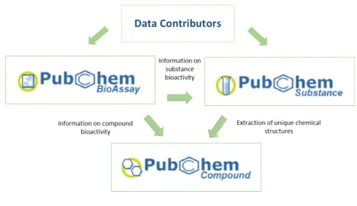
These databases provide different information, with the Substance database containing the chemical information for the substances submitted by the various data contributors while the Compound database stores the information regarding the unique chemical structures derived from the submitted substances through the PubChem standardization process (S. Kim et al., 2016). In the Bioassay database is stored the information about the individual Bioassays, that is, about the studies performed to determine the bioactivity of molecules on a specific target, and the respective results, providing datasets with the tested compounds and their classification as active or inactive (Y. Wang et al., 2014). The substances, compounds, and bioassays included in PubChem’s databases all have unique identifiers, respectively: SID (Substance ID), CID (Compound ID), and AID (Assay ID) (S. Kim, 2016). The origin and organization of PubChem’s data are presented in the following figure: Figure 1 - PubChem Structure There are several features that make PubChem a valuable resource for the implementation of virtual screening and subsequent physical testing of the compounds of interest identified (Kim, 2016):

• The complementary bioactivity information to the bioassay data that is extracted from scientific articles and is provided by contributors that include ChEMBL (Bento et al., 2014), PDBbind (Liu et al., 2015), BindingDB (Gilson et al., 2016), and IUPHAR/BPS Guide to Pharmacology (Southan et al., 2016).

• The availability of compound related information that complements the bioactivity data. This includes properties of FDA approved and investigational drugs provided by DrugBank (Law et al., 2014) such as their indications, mechanisms of action, target macromolecules, interactions with proteins and genes, and ADMET properties; toxicology data provided by the Hazardous Substances Data Bank (Fonger, Hakkinen, Jordan, & Publicker, 2014) and 3-D structures of small molecules provided by the Molecular Modelling Database (Madej et al., 2014); • Assurance of compound availability for subsequent testing. There is always at least one data contributor for each compound in PubChem who claims to have it. If the compound becomes unavailable for whatever reason, it becomes nonlive, meaning that it cannot be searched but is still present in the database. Data Contributors

5 • Easy identification of existent patents for compounds. Given the importance of being able to patent potential drugs in research programs, PubChem offers links between patent documents from U.S., Europe and Word Intellectual Property Organization (WIPO) and unique chemical structures. • Possibility of inferring, for less studied compounds, their chemical characteristics through the comparison with structurally similar compounds. PubChem makes this process easier by providing a precomputed list of such molecules, called “neighbors”. This similarity can be computed in relation to 2-D or 3-D characteristics, giving rise to 2-D or 3-D neighbors. • Programmatic access to PubChem. There are several programmatic ways by which it is possible to access PubChem’s data. These include Entrez Utilities, Power User Gateway (PUG), PUG-SOAP, and PUG-REST. It is also possible to download the databases in different file formats including XML and SDF (Spatial Data File – a type of chemical data file format) through the File Transfer Protocol.

2.2.

R

EVIEW OF WORKS USING VIRTUAL SCREENING

There have been several published works where virtual screening of PubChem was performed with different approaches. Here will be mentioned the ones found most relevant in terms of similarity of objectives with the study at hand. Chen and Wild (2010) have conducted a study where a Naïve Bayes model was created to predict activity using 1133 bioassays from the PubChem database. A particular type of molecular fingerprints (FCFP_6 circular) and their encoded structural features were used for the model creation. The authors concluded that Bayesian models generated from PubChem Datasets are reasonably accurate but that the variability in their accuracy is still quite higher than that observed in the more traditional QSAR (Quantitative Structure-Activity Relationship) modeling used for drug research (Cherkasov et al., 2014). This fact makes them suitable for virtual screening where the main objective is to obtain a smaller number of potentially active compounds to be tested, but not for prediction where high levels of accuracy are needed. The authors point that a way to improve the accuracy would be to include more information about inactive compounds. (Chen & Wild, 2010)

In 2008, Weis, Visco and Faulon (2008) developed a Support Vector Machine (SVM) classifier to identify compounds that act as Factor XIa inhibitors. The classifier was trained on one of the bioassays conducted for the identification of Factor XIa inhibitors, using the Signature molecular descriptor. The bioassay used was chosen considering two factors: the fact that it was a confirmatory assay which diminishes the number of false positives present and that it had a balanced number of positive and negative compounds which eliminates a problem that is common in HTS data. This problem resides in the fact that the sets are usually highly imbalanced with a much smaller number of active than inactive compounds, leading to classifiers that may have high accuracy but are unable to identify the positive compounds, a problem that will also be further mentioned in this study. After implementation of the authors’ version of recursive cluster elimination for feature selection, the final model’s 10-fold cross-validation accuracy was improved from that of a random classifier to 89%, proving its adequacy for the

6 usage in the case at hand. It was also used to screen the 12 million compounds that were present at the time in PubChem’s database. (Weis, Visco, & Faulon, 2008) Han et al. (2012), evaluated Support Vector Machines for the identification of Src inhibitors in large compound libraries by training and testing the models on 1703 inhibitors and 63318 putative non-inhibitors reported before 2011, with the result of correctly identifying 93.53%~ 95.01% inhibitors and 99.81%~ 99.90% non-inhibitors, in 5-fold cross validation studies. The model correctly identified 70.45% of the 44 inhibitors reported since 2011, with the model being applied both to the complete PubChem database and the MDDR database (A bioactivity database produced by BIOVIA and Thomson Reuters with information gathered from patent literature, journals, meetings, and congresses (“BIOVIA Databases | Bioactivity Databases: MDDR,” n.d.)). (B. Han et al., 2012) A study to predict activity against parasitic nematodes was conducted by Khanna and Ranganathan (2011) where a Support Vector Machine model was trained using data from various sources including PubChem to gather the active compounds, while the inactive compound set was derived from DrugBank (Law et al., 2014). The validation of each model was done using ten-fold stratified cross-validation and the best results, with an accuracy of 81.79% on an independent test set, were obtained using the radial basis function kernel. The authors concluded that the developed model would be able to identify new potentially anthelmintic active compounds. (Khanna & Ranganathan, 2011)

Prediction of activity on human ether-a-go-go related gene (hERG) potassium ion channel was performed by Shen, Su, Esposito, Hopfinger and Tseng (2011) using an SVM model and different hERG Bioassay datasets for training and validation, while a test set was derived from literature data. The evaluation was performed with 10-fold cross-validation, and the best model had an accuracy, sensitivity, and specificity of 95%, 90% and 96%, respectively and an overall accuracy for the testing set of 87%. The conclusions drawn by the authors were that the model was able to predict “predisposition” to block hERG ion channels and that it was robust across the structural diversity of the training set. (Shen, Su, Esposito, Hopfinger, & Tseng, 2011) Cheng et al. (2011) conducted a study to identify inhibitory activity of compounds on cytochrome P450 (CYP) since its inhibition is an important factor in drug-drug interactions. For this purpose, the authors used a data set composed of 24700 compounds extracted from PubChem and a combined classifier algorithm. This algorithm is an ensemble of different independent machine learning classifiers: Support Vector Machine, C4.5 Decision Tree, !-Nearest Neighbors And Naïve Bayes, fused by a back-propagation Neural Network. The models were validated by 5-fold cross-validation and separate validation set. The results obtained led to the conclusion that these models are applicable to the virtual screening of inhibitors of the different isoforms of CYP. (Cheng et al., 2011)

Another study to predict inhibitory activity on CYP was conducted by Su et al. (2015). The authors used a rule-based C5.0 algorithm and different descriptors, including, amongst others, PubChem’s Substructure fingerprints. An algorithm of rational sampling was also developed to select compounds from the training set in order to enhance the performance of the models. The optimized model showed improvements in relation to previously existing models, being useful for the screening of large data sets of compounds and also providing the most important rules to identify probable inhibitors which can give new insights about the structural features that are important for this activity. (Su et al., 2015)

7

Han, Wang and Bryant (2008) developed Decision Tree (DT) models to predict activity of 5HT1a agonists, antagonists, and HIV-1 RT-RNase H inhibitors using PubChem Bioassay data and compound fingerprints. The models were evaluated by 10-fold cross-validation and obtained sensitivity, specificity and Mathews Correlation Coefficient (MCC) in the ranges 57.2%-80.5%, 97.3%-99.0% and 0.4-0.5 respectively, with the conclusion that the DT models developed can be used for virtual screening as well as a complement to other more traditional approaches to activity prediction. (L. Han, Wang, & Bryant, 2008)

Schierz (2009) used Weka’s (Hall et al., 2009) cost-sensitive implementation of four classifiers (Support Vector Machines, C4.5 Decision Tree, Naïve Bayes And Random Forest) that were applied to data from several Bioassays on different targets. The authors concluded that Weka's implementations of the Support Vector Machine and C4.5 Decision Tree learner performed relatively well and that care should be taken with the use of primary screenings for their high number of false positives as well as with the use of Weka’s cost-sensitive classifiers as “across the board misclassification costs based on class ratios should not be used when comparing differing classifiers for the same dataset.” (Schierz, 2009, p. 21) A consensus model using the !-Nearest Neighbor algorithm was developed by Chavan, Abdelaziz, Wiklander and Nicholls (2016) for the classification of hERG potassium channel blockers. The authors first constructed 8 models based on 8 different kinds of signatures, one of which was PubChem’s Substructure Signature, that were obtained for a data set of 172 channel blockers that was created based on information retrieved from OCHEM (“Online Chemical Modeling Environment,” n.d.) and Fenichel (“Receptor Binding,” n.d.). The authors then created consensus models based on majority rule and on the sensitivity of the individual models (as in this case it was more important the ability to identify active compounds) using 3, 5 and 7 different signatures. The final consensus model showed sensitivity and specificity of 0.78 and 0.61 for the internal dataset compounds and 0.63 and 0.54 for an external validation set of PubChem data. (Chavan, Abdelaziz, Wiklander, & Nicholls, 2016)

Wang, Xie, Wang, Zhu and Niu (2016) applied four different Machine Learning algorithms to the prediction of selective estrogen receptor beta (ER-b) agonist activity: Naïve Bays, !-Nearest Neighbor, Random Forest and Support Vector Machine. The data about the active chemical structures was retrieved from public chemogenomics databases and five types of chemical descriptors were used, including PubChem’s fingerprint. The models were evaluated by 5-fold cross-validation with a reported range of classification accuracies between 77.10% and 88.34%, and a range of area under the ROC (receiver operating characteristic) curve between 0.8151 and 0.9475. The study suggests that the Random Forest and the Support Vector Machine classifiers are more suited for the classification of selective ER-β agonists than the other evaluated classifiers. (S. Wang, Xie, Wang, Zhu, & Niu, 2016) Novotarskyi, Sushko, Körner, Pandey and Tetko (2011) conducted a study that compared different models for their efficacy in predicting bioactivity on CYP1A2. These models were built using various combinations of Machine Learning methods and chemical descriptors. The ML algorithms used were Associative Neural Networks (“a combination of an ensemble of feed-forward neural networks and KNN” (Novotarskyi, Sushko, Körner, Pandey, & Tetko, 2011)), k-Nearest Neighbors, Random Tree, C4.5 Decision Tree and Support Vector Machine with all of the models being also used in combination with the Bagging technique. The different combinations of these methods with the different chemical descriptors and the usage of either the full set of descriptors or a subset of selected ones resulted in 80 evaluated models. The authors concluded that descriptor selection did not improve the quality of

8

the models and that the best performing model was ASNN with the full descriptor set with 83% and 68% of accuracy in the internal and external test sets, respectively. (Novotarskyi et al., 2011)

In a work conducted by Pouliot, Chiang and Butte (2011) the authors built Logistic Regression models with the goal of correlating postmarketing adverse reactions (ADRs) with screening data from PubChem’s Bioassay database. The developed pipeline used 508 BioAssays of the PubChem database with 485 different drug components. The ADRs were grouped in different system organ classes and models were built for each of these. The models were evaluated using Leave One Out Cross-Validation (LOOCV) and the authors report a better performance than expected given the simplicity of the Logistic Regression models with half of the models having an AUC of ³ 0.7 and all of the models having AUC ³ 0.6. (Pouliot, Chiang, & Butte, 2011) Recently, Yu, Shi, Tian, Gao and Li (2017) presented a study with the objective of developing a model for the classification of CYP450 1A2 inhibitors and non-inhibitors using a multi-tiered deep belief network (DBN) on a large dataset. The authors used a dataset of over 13000 compounds from PubChem and 245 molecular descriptors including both 2D and 3D descriptors that were calculated by molecular computational software. With the objective of improving the classifier’s performance and decrease the computational time a descriptor selection was performed by implementation of three rules: removal of descriptors with too many zeros, with small standard deviation values (< 0.5%) and with correlation coefficients higher than 0.9. For comparison purposes, shallow machine learning models were also trained, namely Support Vector Machine and Artificial Neural Network. All models were run several times to determine the best parameters to use and evaluated by 5-fold cross validation and by an external dataset. The best results were obtained by the DBN model using both 2D and 3D descriptors with an internal overall accuracy of 83.6% and an external accuracy of 77.0%. (Yu, Shi, Tian, Gao, & Li, 2017)

In the study by Bilsland et al. (2015), Artificial Neural Networks were used for virtual screening of Selective G1-Phase Benzimidazolone inhibitors. The dataset used was derived from PubChem Bioassay data with the authors opting to reduce the number of inactive compounds by applying similarity filters using chemical software to obtain a balanced dataset. The final training set contained 3924 compounds of which 1859 were active and 2065 were inactive. The descriptors used included PubChem’s fingerprints amongst others, resulting in a group of 2780 features. Successive runs were performed to identify the best parameter selection, to eliminate compounds that were consistently misclassified and to determine the optimal subset of descriptors. The authors opted to use as a final model an ensemble of 10 networks trained using the optimal combination of parameters, compounds and descriptor set. The overall sensitivity, specificity and accuracy evaluated by 10-fold cross validation were, respectively, 83.1%, 82.4% and 82.7% with the authors considering these results to indicate very good predictive performance. (Bilsland et al., 2015) While most of the QSAR studies for this target have used regression techniques, the works described below have used classification models to predict the inhibitory activity of compounds on EGFR: In the work published by Kong, Qu, Chen, Gong and Yan (2016) the authors have developed models for the classification of compounds as inhibitors or non-inhibitors of EGFR by using Kohonen’s Self-Organizing Map (SOM) and Support Vector Machine (SVM) algorithms. The used dataset was compiled from CHEMBL (Bento et al., 2014) keeping only the compounds with inhibitory concentration (IC50) under 10 µM, resulting in 1248 inhibitors. For the inactive compounds 3093 decoys where gathered

9

from the DUD database (Huang, Shoichet, & Irwin, 2006). A PCA analysis was performed on some properties to determine that there was overlapping in the active and inactive compounds as to make the identification challenging. The final dataset was divided into training and test set to perform evaluation of the model. For the molecular descriptors, ADRIANA.Code (Gasteiger†, 2006) descriptors were calculated and then a subset selected based on correlation with activity. The authors reported that the final models had prediction accuracies on training and testing set, respectively, of 98.5% and 96.3% for the SOM model and 99.0% and 97.0% for the SVM model, and sensitivity, specificity and MCC, respectively, of 94.0%, 97,3% and 0.91 for the SOM model and 94.2%, 98.2% and 0.93 for the SVM model, concluding that both models had good performance when distinguishing between inhibitors and decoys of EGFR. (Kong, Qu, Chen, Gong, & Yan, 2016)

Zhao et al. (2017) conducted a recently published study where the authors constructed 2D and 3D-QSAR models with the 2D model being built using a Support Vector Machine classifier. The used dataset was constructed using 100 inhibitors retrieved from the literature and 185 inhibitors from the DUD database. For the 2D study the dataset was divided into three training sets which accounted for

75%, 70% and 50% of the whole dataset. Forty-five molecular descriptors where calculated using ChemOffice (Irwin*, 2005) and a subset of 9 descriptors was selected using Correlation-Based Feature Selection combined with Genetic Search algorithms. The training of the model was conducted with the three different training sets with the authors opting to use the dataset accounting for 70% of the data which led to the higher accuracy. The final model presented sensitivity, specificity, accuracy and MCC of 98.55%, 99.23%, 98,99% and 0.978, respectively on the training set evaluated by ten-fold cross-validation and 96.77%, 98.18%, 97.67% and 0.950 on the test set, indicating good performance of the model. (Zhao et al., 2017) Singh et al. (2015) developed a model for the classification of compounds as inhibitors or non-inhibitors of EGFR. For this purpose, the authors obtained 3528 anti-EGFR compounds and their inhibitory concentration (IC50) from a database that was also developed by the authors and that contains

information gathered from around 350 research articles. With these compounds, the authors built three different data sets with different proportions of active and inactive compounds according to the chosen IC50 level threshold: EGFR10, EGFR100, EGFR1000. As the chemical descriptor, the authors used

PubChem’s Substructure fingerprints calculated for the compounds present in the datasets built by the authors. Each of the datasets was divided into training and validation sets for the purpose of model evaluation and different ML algorithms implemented in Weka were applied, including IBK (an implementation of !-Nearest Neighbors), Naïve Bayes, Support Vector Machine and Random Forest. The authors found that the best performing model was the Random Forest with an accuracy, sensitivity, specificity, and MCC of 83.66%, 69.89%, 86.03% and 0.49, respectively, when evaluated on the EGFR10 dataset which had the lowest threshold of IC50 and thus a smaller proportion of active

compounds. (Singh et al., 2015)

2.3.

E

PIDERMAL

G

ROWTH

F

ACTOR

R

ECEPTOR

(EGFR)

The Epidermal Growth Factor Receptor (EGFR) or erbB1/HER1 is a transmembrane glycoprotein (Herbst, 2004). It is a member of the erbB/human epidermal growth factor receptor family of tyrosine kinases, which also includes erbB2/HER2, erbB3/HER3 and erbB4/HER4 (Troiani et al., 2012). EGFR is found not only in the plasma membrane, but its expression levels are also high in the nucleus, endosomes, lysosomes, and mitochondria (H. Li, You, Xie, Pan, & Han, 2017).

10

The EGFR signaling pathway is of extreme importance in mammalian cells, having roles in growth, survival, proliferation, and differentiation of cells (Oda, Matsuoka, Funahashi, & Kitano, 2005). It is also overexpressed in a variety of cancers: EGFR is overexpressed in 50–80% of non-small cell lung cancers and ErbB2 and ErbB3 are overexpressed in 25–30% and 63% of breast cancers, respectively (Scharadin et al., 2017). It is also related to increasing resistance to chemotherapy and radiation therapy of tumor cells (Herbst, 2004), and is overexpressed in cancers of very poor prognosis such as pancreatic cancer (Troiani et al., 2012) making it a critical drug target, being its inhibition of particular interest. Currently, therapies directed at EGFR are included in two general categories: monoclonal antibodies that target the extracellular domain and small molecule tyrosine kinase inhibitors that show effectiveness but eventually lead to resistance (Scharadin et al., 2017) which justifies that the search for new potential inhibitors is continually necessary.

Because of its high prevalence in a number of pathways both healthy and pathogenic that make it a potential drug target of such importance and of the development of resistance, the research for compounds with bioactivity on this target has been great and continuous since the discovery of its role in cancer in the 1980’s (Vastag, 2005). This has led to the existence of vast literature on the subject which makes data on known inhibitors freely available (Singh et al., 2015).

All the previously mentioned characteristics, mainly the importance as a drug target, the ever-increasing need for new inhibitors driven by resistance, and the availability of data makes EGFR a great target for virtual screening.

2.4.

D

ATA

M

INING AND

M

ACHINE

L

EARNING

A

LGORITHMS

T

HEORETICAL

F

RAMEWORK

The term Data Mining (DM) was initially a derogatory term that meant the act of searching for an insight that was not supported by the data (Leskovec, Rajaraman, & Ullman, 2011). With the increase of readily available data both in quantity and size, it has taken a positive meaning and can be described as a process to discover patterns and relationships in data that can bring previously unknown insights and allow the making of valid predictions (Edelstein, 1999). It results from the crossing of several fields including Database Management, Artificial Intelligence, Machine Learning, Pattern Recognition, and Data Visualization (Friedman & Friedman, 1997). Data Mining has applications in any industry. These applications include customer segmentation and targeting, credit scoring, fraud detection and drug effect identification in drug trials (“Data Mining From A to Z,” n.d.). Some authors consider Data Mining and Machine Learning (ML) as synonyms and Data Mining does use algorithms from ML in its processes of Knowledge discovery (Leskovec et al., 2011). But Machine Learning can be said to be the discipline that aims at making computers modify or adapt their actions (which can be making predictions or others) so that these actions become more accurate in terms of the goal (Marsland, 2015) using metrics that evaluate this adaptation to guide the process. When it comes to the kind of tasks related to Data Science, we can say that Machine Learning refers to the creation and use of models that are learned from Data, which will typically have as a goal the prediction of a certain outcome (Grus, 2015). In the last decade, the multidisciplinary nature of Machine Learning has become apparent. Concepts from Neuroscience and Biology, Statistics, Mathematics and Physics have all contributed to the development of processes to make computers learn (Marsland, 2015), which is apparent in algorithms

11 such as Artificial Neural Networks (Rumelhart, Widrow, & Lehr, 1994), and Genetic algorithms (Koza, 1992).

2.4.1. Types of Data Mining Problems

2.4.1.1. Regression/Classification Problems

Data mining problems can be classified as either Regression or Classification problems. Both the input and predicted variables used to develop a model can be either quantitative or categorical. In a general sense, we can say that a problem that aims to predict a quantitative value is a Regression problem while problems that aim to assign a record to a certain category are Classification problems (James, Witten, Hastie, & Tibshirani, 2013).

2.4.1.2. Types of Learning

Data Mining problems can also be classified in terms of the amount and type of supervision they get during training. These include: • Supervised Learning: A training set of records with their correct responses (targets or labels) is provided (Marsland, 2015). In this case, the aim is to fit a model that relates the predictors with the response, in order to be able to predict the response for new observations (prediction) and/or to better understand the relationship between the response and the predictors (inference) (James et al., 2013). • Unsupervised Learning: On the other hand, in unsupervised learning, the training dataset does not include labels for a target variable, and in this case, the aim is to find relationships between the variables or between the observations (James et al., 2013). • Semi-supervised Learning: In this kind of learning there is a large amount of unlabeled data and a smaller amount of labeled data. Most semi-supervised systems consist of combinations of supervised and unsupervised algorithms (Géron, 2017). • Evolutionary Learning: Learning systems inspired by biological evolution using the concept of fitness as a measure of how good is the current solution (Marsland, 2015). • Reinforcement Learning: In reinforcement learning the algorithm is told when the answer is wrong but not how to get the right one. In this case, the algorithm or agent can observe the environment and experiment with different solutions that get rewarded, with the agent having to figure out which is the best policy to increase these rewards (Géron, 2017; Marsland, 2015). In this study, the problem at hand is a Classification problem with supervised learning since the objective is to classify the compounds in PubChem’s database or others as either active or inactive and the algorithms used will be provided with the correct category for the training examples.

12

2.4.2. Theoretical background of the used algorithms

2.4.2.1. Decision Trees

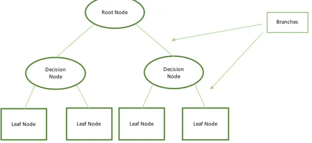
A simple way to describe Decision Trees is that they are a way of representing a set of rules that when applied to an observation can lead to a class or value (Edelstein, 1999). They are composed of a root node, decision nodes and leaf nodes that are connected by branches: Figure 2 - Decision Tree Structure At the root (the first split) and at the decision nodes, each attribute is evaluated according to a rule which is applied in each branch until a leaf node is reached where there are no more attributes to evaluate on (Daniel T. Larose, 2015). The greater the purity of the leaf nodes and the distance between them the better (Edelstein, 1999). Decision Trees have the advantages of being simple and allowing easy interpretation, but usually don’t perform as well as other more complex algorithms in terms of accuracy (James et al., 2013) and overfit to the training set very easily which means less generalization capacity (Grus, 2015). In the process of building decision trees, it is necessary to determine which questions are being asked in each decision node and in what order (Grus, 2015). To achieve this goal, it is necessary to have measures of purity of the nodes before and after the partition is applied and to calculate that difference which will be the measure of how much information will be gained by applying a certain partition. The two most used measures for this purpose are Entropy and Gini Impurity (Marsland, 2015): • Entropy of a set of probabilities #$: %&'()#* = − #$log1#$ $ 1 • Gini Impurity for a particular feature k: 34 = 1 − 7$895 6 1, 2 Root Node Decision Node Decision Node Leaf Node

Leaf Node Leaf Node Leaf Node

13

where c is the total number of classes and N(i) is the fraction of records that belong to class i.

Trees that are allowed to grow indefinitely will overfit to the training data. In order to avoid this, stopping rules must be applied. Common stopping rules are simply limiting the maximum depth that the tree can reach or establishing a lower limit to the number of records in a node. Alternatively, it is possible to prune the tree, where the tree is allowed to grow to full size and then is pruned back to the smallest size that does not compromise accuracy. (Edelstein, 1999) There are different algorithms that can be used to build a tree that include ID3, C4.5, C5.0, and CART. In this work, the algorithm used is CART. The CART algorithm produces binary trees, that is, for each feature, it splits the training set into two subsets based on a certain threshold value for that feature. The feature and threshold used are chosen so that the purest subsets are obtained. It follows these steps recursively until the stopping condition is met. CART is a greedy algorithm which means that the optimum splitting choice is made at each level without checking if it will lead to the purest subsets in the levels below. This usually leads to a good solution but doesn’t guaranty an optimal one (Géron, 2017).

2.4.2.2. Naïve Bayes

Studies have found the Naïve Bayes classifier to have comparable performance to Decision Trees and some Neural Network classifiers (J. Han, Kamber, & Pei, 2012). It is called Naïve Bayes because it assumes that the observation variables are independent of each other which will most of the times not be true. This classifier is based on Bayes’ theorem that states that (Marsland, 2015):

@ A B = @ B A @ A

@ B , 3

where @ A B is the conditional probability of H given X, @ B A is the conditional probability of X given H and @ A and @ B are the a priori probabilities of H and X, respectively. For the purpose of classifiers, we can consider @ A to be the probability of the hypothesis that the observation X belongs to a certain class, and @ B the probability that an observation X is equal to a certain vector of variables.

With the use of the assumption of independence of the variables in the dataset, we come to a simplified equation that states that the probability of an observation Xj being equal to a certain vector

of variables given that it belongs to class D$ (@ BE D$ = @(BE9, BE1, … BEG|D$), where the superscripts

of X represent the index of the variables of the vector), is equal to the product of the individual probabilities: @ B_E4 _{= I} 4 D$ J = @ BE9= I9 D$ × @ BE1= I1D$ × … × @ BEG= IG D$ , 4 and the classifier will select the class D$ for which the following computation is the maximum: @(D$) @(BE4 = I4|D$ 4 ). ₅ Although this computation is the result of an obviously incorrect assumption, several empirical studies

14

show that Bayesian classifiers perform well and are comparable to other more complex algorithms (J. Han et al., 2012) as the assumption made tends to not hurt classification performance (Foster & Fawcett, 2013). This classifier is very efficient in terms of used storage space and computational time and it is also a natural “incremental learner” as it can update its model one example at a time without having to reprocess all past training examples (Foster & Fawcett, 2013). In theory, Bayesian classifiers will have the minimum error rate in comparison to other models which not always happens in practice due to the inaccuracies resulting from the assumptions made (J. Han et al., 2012). Nonetheless, it is a very commonly used classifier to serve as a baseline to which other models are compared (Foster & Fawcett, 2013).

2.4.2.3. Logistic Regression

Linear Regression aims to approximate the relationship that exists between a set of variables and a continuous response, but when the response is categorical Linear Regression is not applicable. However, an analogous method can be used, Logistic Regression (Daniel T. Larose, 2015). It is mostly used to predict binary variables but can also be applied to the prediction of multi-class variables (Edelstein, 1999). In a classification problem, we want the examples that are further away from the boundary between classes to have a higher probability of belonging to that class. The problem of using Linear Regression is that the distance from the border can range from −∞ to +∞ while the probabilities should be in the range zero to one (Foster & Fawcett, 2013). Since the target variable is discrete and it is not possible to directly model using linear regression, instead of predicting if the event itself will happen the logistic model predicts the logarithm of the odds of its occurrence (Edelstein, 1999). To meet the objective of getting probabilities between zero and one we can use the logistic function (James et al., 2013): # B = ℯRSTRUV 1 + ℯRSTRUV, 6

where the XY and X9, represent the coefficients for a single predictor X.

With some manipulation of the formula we arrive at: log # B 1 − # B = XY+ X9B , 7 with the left side being the log-odds or logit that is linear to X. For a regression with multiple predictors the previous equation can be generalized to: log # B 1 − # B = XY+ X9B9+ ⋯ + X\B\. 8

15

To estimate the coefficients in the logistic regression model, the maximum likelihood method is used, where the coefficients sought are the ones that will make the predicted probability of each individual be as close as possible to their actual observed category. This can be formalized in the following equation called a likelihood function where the estimates XY and X9 are chosen to maximize the

following function (James et al., 2013): ^ XY, X9 = # _$ 1 − # _$` $`_:b c`8Y $:bc89 . 9 Logistic Regression is a very powerful modeling tool, but it does assume that the target variable (the log odds) is linear in the coefficients of the predictor variables. Also, the optimization of the model may depend on the choice of the right inputs and their functional relationship to the target variable by the modeler, who would also have to explicitly add terms for any possible interactions which requires skill and experience of the analyst (Edelstein, 1999).

2.4.2.4. k-Nearest Neighbors

The k-Nearest Neighbors (k-NN) algorithm uses the similarity between examples to classify them. It places an example in the class to which most of their neighbors belong to (Edelstein, 1999). Each of the training records described by n attributes represents a point in an n-dimensional space. When presented with a new example, the classifier searches the pattern space for the ! examples that are closer to it. For this purpose, it is necessary to have a measure of distance between the training records. The most commonly used distance measure is the Euclidean distance that can be represented by (J. Han et al., 2012): e6f' B9, B1 = _9$− _1$ 1 G $89 , 9

where B9 and B1 are two points represented by the tuples: B9 = (_99, _91, … , _9G) and B1 =

(_19, _11, … , _1G). The determination of which class to assign the new example to can be made by voting, that is, assigning the new example to the class where the majority of its k neighbors belong to, as previously described, or it can be determined by averaging the values of its k nearest neighbors which gives an estimate of the probability of the example belonging to that class. It is also possible to use weighted voting where the most distant neighbors will be assigned a smaller weight than the closer ones (Foster & Fawcett, 2013). There is no direct answer to what the value k should be, although odd numbers are advantageous for majority voting purpose. A too small value of k will make the classifier too sensitive to noise while a value that is too large will reduce accuracy as points that are very far from the example will be considered (Marsland, 2015). The most common approach would be determining it experimentally by running the model with several incremental values of k and using the k that gives the lowest error rate on the testing set (J. Han et al., 2012).

16 k-NN models have a large computational load because the calculation time increases as the factorial of the total number of points. It is necessary to make a new calculation for each new presented case. On the other hand, they are very easy to understand when there are few predictor variables and are useful for non-standard data types, such as text, as it is only required the existence of an appropriate metric. (Edelstein, 1999)

2.4.2.5. Support Vector Machine

Support Vector Machine (SVM) is an algorithm that can be used to classify both linear and nonlinear data. It works by applying a nonlinear mapping to transform the original dataset into a higher dimension where it searches for the linear optimal separating hyperplane, the maximum margin hyperplane. This hyperplane is determined by using support vectors and the margins that they define (J. Han et al., 2012).

Linearly Separable Data

For data that has linearly separable classes, an hyperplane exists that classifies all instances correctly and the maximum margin hyperplane will be the one that achieves this and gives the greatest separation between the classes (J. Han et al., 2012).

A hyperplane separating two classes can be expressed by:

0 = hY+ h9I9+ h1I1, 10

in a case with two attributes I9 and I1 and three weights to be determined.

Adjusting this equation to the hyperplanes that define the limits of the margin we get: A9: hY+ h9I9+ h1I1 ≥ 1 for *$ = 1 11 A1: hY+ h9I9+ h1I1 ≤ 1 for *$ = −1 12 Or, combining the two inequalities: *$ hY+ h9I9+ h1I1 ≥ 1, ∀$ 13 The instances located on the hyperplanes that define the margins are called Support Vectors, and for each class, there is always at least one. They are located at the same distance from the maximum margin hyperplane and are the most important in terms of the classification, since after being defined all other instances could be removed and the model would still be the same (Witten & Frank, 2005).

17 Figure 3 - Representation of Maximum Marginal Hyperplane The maximum margin hyperplane equation can be given by: _ = n + o$*$I 6 ∙ I 14

where *$ is the class value of training instance I 6 , n and o$ are parameters determined by the fitting

of the algorithm, and the term I 6 ∙ I represents the dot product of a test instance with one of the support vectors, and so we achieve a constrained quadratic optimization problem (Witten & Frank, 2005). Non-linearly Separable Data To apply SVMs to nonlinear data, an extension of the linear approach can be used where the original data is transformed into a higher dimensional space by applying real functions q on an input vector, where the algorithm will search for a linear separating hyperplane that corresponds to a nonlinear separating hypersurface in the original space (J. Han et al., 2012). This computation is very expensive as the dot product involves one multiplication and one addition for each attribute and the total number of attributes in the new space can be immense (Witten & Frank, 2005). However, instead of computing the dot product on the transformed input vectors, it is mathematically equivalent to apply a kernel function r(B$, BE) to the original input as in:

r B$, BE = q B$ ∙ q BE , 15

where q B is the nonlinear mapping function used to transform the training tuples.

18

As such, the dot products can be substituted by one of the less computationally expensive kernel functions that include the following (J. Han et al., 2012): • Polynomial kernel of degree h: r B$, BE = B$∙ BE+ 1 s 16 • Gaussian radial basis function kernel: r B$, BE = ℯt VctVu v 1wv ₁₇ • Sigmoid kernel: r B$, BE = tanh |B$∙ BE− } 18 Support Vector Machines are very useful as they produce very accurate classifiers but are quite slow when compared to other algorithms (Witten & Frank, 2005) and, as such, it is a major research goal to make SMVs faster both in the training and testing phases, so that they can be more easily applied to very large datasets (J. Han et al., 2012).

2.4.2.6. Neural Networks

Artificial Neural Networks are predictive models inspired by the way the brain works. The brain is composed of neurons wired together where each neuron receives inputs from other neurons and (according to the activation threshold) either fires and produces a response to other neurons or doesn’t (Grus, 2015).

Neural Networks are algorithms that are efficient in the modeling of large and complex problems and that may be used both in classification and regression problems (Edelstein, 1999). They were first introduced in the 60’s, and since then there have been several waves of new interest towards them (Géron, 2017). The simplest implementation of a Neural Network is a Perceptron. It is composed of an input layer with one node for each input variable and an output layer where each node is connected to all nodes in the input layer and, usually, a bias feature. The perceptron calculates a weighted sum of the input vector and then applies a step function to the result of the sum and outputs that result. The most commonly used step function is the Heaviside step function (Géron, 2017): A~I6f6e~ Ä = 0 6Å Ä < 0_{1 6Å Ä ≥ 0} 19 The Perceptron is trained by making a prediction for each example and, after comparing the result with the target, increasing the weights from the inputs that would have contributed to the right prediction. Perceptrons are capable of solving simple linear binary classification problems but are unable to solve some other trivial problems such as the XOR problem (Géron, 2017).

However, some limitations of the Perceptron can be eliminated by stacking multiple Perceptrons giving rise to what is called a Multilayer Perceptron (Géron, 2017):

19 Figure 4 - Simplified representation of Multilayer Perceptron, where Wij is the weight between units i and j and qj is the bias of unit j In the case of the Multilayer Perceptron, one or more hidden layers are located between the input and the output layers, where each node is connected to all the nodes in the previous layer and calculates the weighted sum of the inputs. Each output unit applies a nonlinear activation function to the result of its weighted input. The number of hidden layers and the number of neurons in each layer define the topology of the network. There are no simple rules to determine the best topology for a particular problem and the approach to determine it is experimental (J. Han et al., 2012).

The training of Multilayer Perceptrons is made by the Backpropagation algorithm that consists of several steps that are described next (J. Han et al., 2012): 1. The first step is the initialization of the weights which are small numbers randomly selected. 2. Forward propagation: After the inputs are passed through the input layer, the input and output of each unit in the hidden layer are computed. The net input of the hidden and output layers is computed as a linear combination of its inputs É_E = h_$E $ Ñ_$+ Ö_E, ₂₀

where ÉE is the net input, Ñ$ is the output from the previous unit, h$E is the weight of the

connection between the previous unit 6 and the current unit Ü, and ÖE is the bias of the current unit Ü. ! " Input layer Hidden layer Output layer #_$% &%

20 3. Application of the activation function: Each unit in the hidden and output layers applies the activation function to its net input. Most commonly the logistic or sigmoid functions are used, and this step allows the algorithm to classify nonlinear data. It is also referred to as a smashing function as it smashes a wide range input into values between 0 and 1. This produces the output of the unit and in the case of the output layer, gives the prediction of the network. 4. Error backpropagation: The goal of the backpropagation of the error is to update both the weights and the biases to reflect the error made in the network’s prediction. The error of a unit in the output layer is given by: %((E= ÑE 1 − ÑE áE− ÑE , 21

where ÑE is the actual output of unit Ü and áE is the target value for the particular example. The

error of a hidden unit Ü is given by:

%((_E = Ñ_E 1 − Ñ_E %((₄h_E4

4

, ₂₂

where hE4 is the weight of the connection from unit Ü to unit ! in the next layer and %((4 is

the error of unit !. 5. Update weights and biases. Weights are updated by applying: Δh_$E = ^ %((_EÑ_$ 23 h$E= h$E+ Δh$E 24 where ^ is the learning rate that is used to avoid the algorithm getting stuck on a local optimum. Biases are updated by applying: ∆ÖE= ^ %((E 25 Ö_E= Ö_E+ ∆Ö_E 26 In this case weights are being updated for each example which is called case updating, but they can also be stored in a variable and be updated after all the examples in the training set have been presented to the network, which is called epoch updating, as one iteration through the training set is named an epoch. 6. Termination of the algorithm: The training stops when a termination condition is met. This can be either when the weights of the previous epoch or the error of the network are below a certain specified value, or when a specified number of epochs have been run.

Although Neural Networks are versatile, powerful, scalable and appropriate for large and highly complex tasks (Géron, 2017), they have some disadvantages. These include their tendency to overfit, the fact that they are nearly impossible to interpret, being what is called a “black box”, and that they

21 have a long training time, although the predictions are provided quickly (Edelstein, 1999).

2.4.2.7. Ensemble methods

Ensemble methods are based on a principle similar to that of the wisdom of the crowd which is a phenomenon where the average answer of a large number of people to a certain question is often better than the single answer of an expert (Géron, 2017).

An ensemble model for classification is a composite model that results from combining different classifiers. Ensemble classifiers tend to perform better than their composing models individually (J. Han et al., 2012). Voting Classifiers The simplest form of Ensemble methods is the Voting method where the predictions for the individual classifiers are aggregated, and the prediction with the majority of votes from the composing classifiers is the one chosen. This strategy, albeit its simplicity, will generally outperform the best classifier in the ensemble and tends to achieve good performance even if all the composing classifiers are weak learners, that is, only slightly better than random guessing. This happens because of the law of large numbers, that states that over a large number of trials the average result will be close to the expected value. In the case of classifiers, this translates to the fact that if all classifiers have an accuracy of above 50%, as their number increases, the accuracy of the combined models will also increase. (Géron, 2017) Bagging Bagging is a method that also uses majority vote to get the final prediction of the ensemble, but it introduces the variety of classifiers in a different way than described previously. The several individual classifiers are built using the same algorithm but on different samples taken from the original dataset with replacement. This implies that a certain sample will likely exclude some examples and duplicate others from the original dataset. The aim of this process is to decrease a source of error for individual classifiers that arises from the use of a particular training set that is inevitably finite and not completely representative of the whole population. That is, it intends to diminish the variance component of the error of the classifier in the bias-variance trade-off. Because of this, Bagging is usually most useful when used with algorithms that are by themselves unstable, such as Decision Trees. (Witten & Frank, 2005) Boosting In Boosting, weights are assigned to each record and, after a classifier is trained, these weights are updated so that the following classifier will give more importance to the records that were misclassified. In the end, the ensemble chooses the correct prediction based on voting with each classifier’s vote weight being a function of its accuracy. (J. Han et al., 2012)

AdaBoost

The most commonly used algorithm to perform boosting is AdaBoost (from adaptive boosting). It can be described by the following (J. Han et al., 2012):