Does anything beat parametric portfolio policies?

! ! ! ! !

"#$%!&'()*+',!-$&)!

.&/&0$)/+1!.#/)2#3+#!

.#3+1+$%4!

!

!

!

!

5+)&!67,&3*#!8+9&%!:&3#1*&!

!

!

!

!

"+%%$/)&)+#'!;/+))$'!7'9$/!)*$!%7<$/=+%+#'!#2!6/7'#!:$/&/9!

!

!

!

"+%%$/)&)+#'!%7-0+))$9!+'!<&/)+&3!2732+30$')!#2!/$>7+/$0$')%!2#/!)*$!?@1!+'!

A+'&'1$!&)!)*$!B'+=$/%+9&9$!C&)D3+1&!.#/)7,7$%&E!F7,7%)!GH

_E!IJHKL!

!

!

!

!

Abstract

This thesis’ objective is to test the parametric portfolio policies (PPP) approach to asset allocation developed by Brandt, Santa-Clara and Valkanov (2009) on an investment universe of large stocks. I enlarge the number of conditional variables to include volatility and tail risk alongside value, size and momentum. I introduce a novel approach by using industry specific standardization when normalizing the characteristics. I also model the stocks for both the unconstrained and the long-only portfolio of stocks. Using a power utility function as representative of the investor’s preferences I test this approach using the Standard & Poor’s 500 as a market proxy. I include a sensibility analysis to different risk aversion coefficients. I conclude that despite the overall good performance of this strategy it should not be seen as a way to hedge the market exposure, but as a way to ’ride’ the market with high risk adjusted returns. I find that an investor always prefers small stocks and past winners. The preference between value and growth stocks depends on the models specifications.

Resumo

O objectivo desta tese é testar o método de alocação de riqueza desenvolvido por Brandt, Santa-Clara e Valkanov (2009) num universo de acções grandes. Além de incluir as variáveis propostas – value, size and momentum – incluo também volatilidade e risco de cauda. Inovo a normalização das características usando estatísticas específicas de cada divisão através do SIC Code. Também modelo a alocação para incluir só posições longas nas acções. Uso uma power

utility function como representativa das preferências de risco do investidor e testo a estratégia

usando o Standard & Poor’s 500 como representante do mercado. Incluo também uma análise de sensibilidade para diferentes coeficientes de aversão ao risco. Concluo, que apesar de no geral a estratégia apresentar boa performance, não deve ser vista pelo investidor como uma forma de alavancar a exposição do mercado, mas sim como uma forma de acompanhar o mercado com retornos ajustados a um risco elevado. Segundo a minha análise um investidor dá mais peso a empresas pequenas e empresas com retorno superior no ano anterior. A preferência entre acções value e growth depende das especificações do modelo.

Content

II. Data Description and Methodology ...8

III. Results ...15

a. Base Case ...16

b. Unconstrained Optimization with Five Characteristics ...20

c. Portfolio Policy with Industry Standardization ...23

d. Constrained Optimization ...25

e. Varying risk aversion ...28

f. Lewellen (2014) Strategy ...30

Table of Figures

Table I – Summary statistics for the characteristics ...9

Figure I – Characteristics mean ...9

Table II – Stock Divisions ...13

Table III – Base Case Portfolio Policy ...16

Figure II – Cumulative portfolio returns ...18

Table IV – Portfolio Policy with Five Characteristics ...20

Table V – Portfolio Policy with Industry Standardization ...23

Table VI – Portfolio Policy with No Short-Sales ...25

Figure III – Cumulative returns for long-only policy portfolio ...27

Table VII – Portfolio Policy with Varying Risk Aversion ...28

Figure IV – Cumulative return of varying risk aversion ...30

I. Introduction

The methods of allocating wealth across the menu of available assets – asset allocation – have long been a topic of great interest in the financial world. Both academics and practitioners devote a large amount of time and effort in applying the academic methods to the real world markets.

Ever since Markowitz (1952) introduced the static mean-variance paradigm, which directly related the trade-off between risk and return, that many other methods have risen. Most academics refer to Markowitz’s paradigm as being computationally intensive, but despite the many shortfalls Brandt (2010) still describes the former as the “de-facto standard in the finance profession”.

During the 1990’s there was a rise in the number of empirical research made in the field of patterns in the cross section of individual stock returns. Even currently, researchers such as Lewellen (2014) defend that the high significance in some patterns makes them almost undoubtedly real and not due to random luck or data snooping.

The uncertainty of the parameters characterizing financial markets is, according to Pástor and Veronesi (2009), erased by the vast quantities of financial data available, but also vulnerable to the randomness that characterizes financial markets. Thus, academic research has for a long time focused on which variables are more relevant in explaining asset returns. Fama and French (1992) start by showing that the market beta does not help explain the cross-section of average stock returns, and proceed to demonstrate that the combination of size and book-to-market ratio are better fit to describe the cross-section of average stock returns. Hanna and Ready (2005) describe the combination of the two characteristics as a “parsimonious characterization of all of the useful information about expected excess returns”.

Lately, more methods have been put into research such as the one presented by Brandt, Santa-Clara and Valkanov (2009) where they introduce a new approach for portfolio optimization with a large number of assets. By only using a limited set of cross-sectional parameters and optimizing the investors’ average utility function the authors provide a computationally simple method of asset allocation. The parameters used are the following firm specific characteristics: size, value and momentum. According to DeMiguel, Garlappi and Uppal (2007), “exploiting information about the cross-section characteristics of assets may be a promising direction to

When considering an investment universe of N stocks, Brandt, Santa-Clara and Valkanov (2009) model only requires the modelling of N weights independently of investors’ preferences while the traditional Markowitz approach involves the modelling of N first and (N2+N)/2 second order moments, which becomes more difficult as N grows larger if we don’t implement different fixes as suggested in Brandt, Santa-Clara and Valkanov (2009) - shrinkage of estimates or imposing a factor structure on the covariance matrix. These fixes require the use of extensive resources and, thus, the methods of portfolio optimization based on firm characteristics are rarely used.

The attractiveness of the method comes from its simplicity. There is no need to compute expected returns as in so many other asset allocation methods. Fama and French (1996) show that these three specific characteristics – value, size, and momentum - are robust proxies for the cross-section of expected returns. The absence of the variance-covariance matrix can be explained by the use of the three characteristics that, according to Chan, Karceski and Lakonishov (1998), hold a relationship with such matrix.

The modelling of the portfolio optimization problem as an utility maximizing one not only simplifies the problem by eliminating the need to use estimators such as the maximum-likelihood one, but also allows the expansion of the model to other asset classes by using characteristics specific to such classes. The estimation of portfolio weights is based on each asset’s characteristics followed by the optimization of the investor’s average utility.

My aim is to build on Brandt, Santa-Clara and Valkanov (2009) by introducing two new variables – volatility and tail risk – and see how this method behaves when considering different firm specific variables than the ones initially tested and compare it to three benchmarks: the naïve portfolio, the value-weighted portfolio and a portfolio created according to the methodology presented by Lewellen (2014), which has a similar approach to the one used by Brandt, Santa-Clara and Valkanov (2009) by also using firm specific characteristics to estimate cross-sectional slopes using Fama-Macbeth regressions. The importance of the comparison between these two methods rests on the fact that both use firm characteristics to maximize the cross-sectional return. The main difference is that while Lewellen (2014) simply maximizes the return not considering the risk of the portfolios held, Brandt, Santa-Clara and Valkanov (2009) maximize the utility, hence, they introduce the risk preference of the investor into the utility maximizing process. Also, using the naïve portfolio as a benchmark is of high significance. DeMiguel, Garlappi and Uppal (2007) compare this portfolio construction method with 14 other different models and none is consistently better in terms of both Sharpe ratio and certainty

equivalent. Although the simplicity of allocation 1/N of our wealth to the different available assets (N) cannot be beaten, I want to compare if there are performance gains in allocating wealth to stocks in a more complex way, as Brandt, Santa-Clara and Valkanov (2009) do. Further, I separate the stocks by industry by using an average and standard deviation of the cross-section of each industry instead of the cross-section statistics of the entire universe of stocks. According to Asness, Porter and Stevens (2001) estimates are more reliable when variables are measured within-industries by reducing measurement error. As an example are the different accounting practices across industries that may lead to differences in the same variable across industries. Subsequently I optimize the investor’s average utility in the same manner as before. My aim is to assess whether sorting stocks into industries and compute cross-sectional statistics accordingly provides extra capital gains for the investor.

The remaining of this thesis is structured as follows: section II described the data used and methodology followed to compute the different strategies, Brandt, Santa-Clara and Valkanov (2009) and its extensions and Lewellen (2014); section III shows the results obtained and compares the different strategies used; section IV concludes.

II. Data Description and Methodology

I use the Center for Research of Security Prices (CRSP) data base for market data and the CRSP-Compustat merged for accounting data. As a proxy for the market index I use US stocks, more precisely the Standard & Poor’s 500 (S&P500) index, which allows me to avoid liquidity concerns. I use the CRSP-Compustat database for the S&P500 from December 1964 to December 2015. To mitigate the effects of survivorship bias I analyze all the stocks that ever belonged to the S&P500 during the time period, therefore including all the stocks that are no longer present in today’s market. I do not exclude the smallest stocks of my sample as the S&P500 includes only large stocks in its listing. I will use the 1-month Treasury-Bill rate from the Kenneth French library as a proxy for the risk free rate.

To compute firm characteristics, I use the approach in Brandt, Santa-Clara and Valkanov (2009). The log of the firm’s market equity is used as the size indicator; the log of the book-to-market ratio represents value, the book value will be lagged six months so the book-to-market can incorporate the fiscal year-end characteristics into the stock price, which, according to Fama and French (1992), is a conservative approach; and the lagged one-year return compounded from t-13 to t-2 as the momentum indicator; in order to avoid the one-month reversal effect t-1 is not included in the computations.

In a given date I only consider stocks for which all characteristics are available. The average sample size is approximately 723 stocks. Its minimum is 499 stocks in the beginning of the analysis, January 1975 and has a maximum of 848 in the month of July 1997. The sample grows 0.035% on average.

To assess the model’s behavior when introducing different characteristics and to check whether its robustness holds I introduce two new conditioning variables: volatility and tail risk. I use the prior 30 day squared variation in daily returns for the former, while the latter will simply be the 95% monthly Value-at-Risk (VaR) measure.

Below I present a table with the summary statistics – mean, median, standard deviation, autocorrelation, skewness and kurtosis – for the five characteristics: value, size, momentum, volatility and tail risk, and also for the monthly stock returns. All the characteristics except returns are winsorized at their 99th percentile. As the focus of this analysis is cross-sectional the values below represent time-series averages of the monthly cross-sectional statistics.

Table I – Summary statistics for the characteristics

The table below presents the mean, median and standard deviation (St.Dev) for the five characteristics: value, size, momentum, volatility, and tail risk. For further analysis, I include skewness (Skew) and kurtosis (Kurt).

Value Momentum Size Volatility Tail Risk

Mean 0.62 0.07 20.86 0.02 0.06

Median 0.49 0.07 20.91 0.00 0.00

St.Dev 0.46 0.30 1.43 0.03 0.08

Skew 1.64 -0.04 -0.23 2.97 1.12

Kurt 7.43 4.09 3.15 13.73 3.25

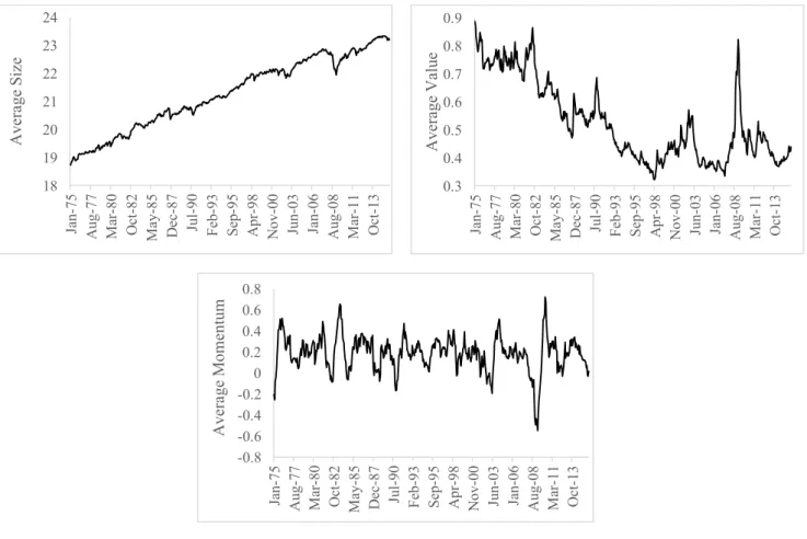
Figure I – Characteristics mean

Figure I below shows the development of the cross-sectional average of the value, size, and momentum characteristics throughout the data sample.

-0.8 -0.6 -0.4 -0.2 0 0.2 0.4 0.6 0.8 Ja n-75 A ug -77 Ma r-80 Oc t-82 Ma y-85 De c-87 Jul -90 Fe b-93 Se p-95 A pr -98 N ov -00 Jun -03 Ja n-06 A ug -08 Ma r-11 Oc t-13 A ve ra ge M om ent um 0.3 0.4 0.5 0.6 0.7 0.8 0.9 Ja n-75 A ug -77 Ma r-80 Oc t-82 Ma y-85 De c-87 Jul -90 Fe b-93 Se p-95 A pr -98 N ov -00 Jun -03 Ja n-06 A ug -08 Ma r-11 Oc t-13 A ve ra ge V al ue 18 19 20 21 22 23 24 Ja n-75 A ug -77 Ma r-80 Oc t-82 Ma y-85 De c-87 Jul -90 Fe b-93 Se p-95 A pr -98 N ov -00 Jun -03 Ja n-06 A ug -08 Ma r-11 Oc t-13 A ve ra ge S iz e

The investor problem is the same as in Brandt, Santa-Clara and Valkanov (2009): choosing the portfolio weights in period t that maximize the investor’s utility in period t+1. The optimal portfolio weights are a linear function of the stocks’ characteristics and are given as follows:

1 𝑤_$,& = 𝑤_(,&+ 1 𝑁&𝜃

,_𝑥 $,&

Where 𝑤(,& is stock’s i weight at time t in the benchmark portfolio, in this case I use the value-weighted market portfolio, 𝜃 is a vector for the parameters associated with the characteristics, and 𝑥_$,& the vector containing the standardized characteristics. The use of the 1/𝑁_& term is to scale the weights of the portfolio and avoid more aggressive allocations as the number of stocks in the sample increases. The standardization of characteristics is, according to Brandt, Santa-Clara and Valkanov (2009), necessary since it solves the non-stationary problem that might arise by using the raw 𝑥_$,&, while also restricts the optimal portfolio weights to sum to one. The investor’s trade-off between risk and return is incorporated in the utility function. I use a power utility function, representative of an investor with isoelastic preferences, with an Arrow-Pratt coefficient of relative risk aversion 𝛾 = 5.

2 𝑈& =

(1 + 𝑚𝑜𝑛𝑡ℎ𝑙𝑦 𝑟𝑒𝑡𝑢𝑟𝑛_&)>?@ 1 − 𝛾

With the understanding of equations (1) and (2) it is easier to interpret the following utility problem:

3 max

[GH,I] 𝐸& 𝑢 𝑟L,&M> = 𝐸&[ 𝑢 𝑤$,&𝑟$,&M>

NI

$O> ]

My aim is to estimate the set of parameters’ coefficients (𝜃) that optimize the portfolio return. It is possible to estimate 𝜃 by maximizing the following:

4 max Q

1

𝑇 𝑢 (𝑤(,&+

1

𝑁_&𝜃,𝑥$,&)𝑟$,&M> NI

$O> ,?>

&OS

I consider both the unconstrained and constrained cases of portfolio optimization. In the former I allow the weights to take any value, while in the latter, the constrained case, I restrict the weights to only positive values, therefore not allowing short selling, hence, creating a long-only equity portfolio. When simply restricting the weights to only take on positive values the optimal portfolio weights no longer sum to one. There is a need to renormalize the portfolio weights. I do so according to the manner presented by Brandt, Santa-Clara and Valkanov (2009):

5 𝑤_$,&M ₌ 𝑚𝑎𝑥 0, 𝑤$,& 𝑚𝑎𝑥 0, 𝑤_V,& NI

VO>

Note that in the unconstrained case I will ignore the margin account regarding short sales, just as Brandt, Santa-Clara and Valkanov (2009) do.

Regarding the performance analysis, I do an in-sample (IS) analysis using the first 10 years of the sample followed by an out-of-sample (OOS) analysis for the remaining dataset using the expanding window method as in Brandt, Santa-Clara, and Valkanov (2009). I will present results for three rebalancing frequencies: annual, semi-annual and quarterly.

Since results, by themselves, are not representative of success I use three benchmarks to assess the strategy’s performance. The first comparison is with the naïve portfolio, which attributes the same weight to every company in the portfolio regardless of their size - 1/N weight in each company. According to DeMiguel, Garlappi and Uppal (2007) the 1/N rule performs better as N grows larger since there is an increase potential for diversification, reducing idiosyncratic risk, among a larger number of stocks. Secondly, I weight each company according to their market capitalization and create a value-weighted portfolio. In this case, portfolio weights are not independent of company size, and larger companies have a larger portfolio weight.

The third and last benchmark used will be the one presented by Jonathan Lewellen in the working paper “The cross section of expected stock returns”. Using Fama-MacBeth (FM) regressions on up to fifteen firm characteristics Lewellen (2004) forecasts monthly returns. Following this measure, the stocks are sorted into portfolios. Regressing on fifteen variables, a relatively large number is to ensure that investors did not know ex ante which variables better suited the predictability of stock returns.

Lewellen (2014) disregards multicollinearity as a concern on the analysis even if some variables are “mechanically related” or “capture related features of the firm”. The argument presented for disregarding such concern is that the main focus of the study is the predictive power of the model and not of the individual characteristics.

This strategy focuses on combining different characteristics to form a portfolio of going long in high expected return stocks and short on stocks with low expected return. These portfolios are created using 12-month rolling averages of Fama-Macbeth slopes. I use a 5-year rolling regression to estimate the betas. Then I run a cross-sectional regression for every time period

Lewellen (2014) creates three models by expanding the firm characteristics used in the first model – size, value, and momentum. My focus here is to compare how different models that use the same set of characteristics but with different methodologies perform. Therefore, I only compute FM regressions for model one as it is the one that most resembles the characteristics used by Brandt, Santa-Clara and Valkanov (2009).

Since the variables used are level or flow variables. The former represents a set of variables that changes slowly over time, and the latter is measured over at least a year. Lewellen (2004) suggests that due to this, predictability might be persistent over longer time periods. I calculate the first three variables – size, value, and momentum – according to the methodology in Brandt, Santa-Clara and Valkanov (2009). This leads to a closer approximation between the two models, Model 1 and the one in Brandt, Santa-Clara and Valkanov (2009), allowing to draw more precise conclusions.

Furthermore, there is one extra specification which I include. For example, the value characteristics depends highly on the practices used by different firms for reporting different accounts in the balance sheet. I try to decrease the errors that the forecast may have, while also assess whether keeping track of which industry a firm belongs to leads to increased performance. According to Asness, Porter and Stevens (2001) estimates are more reliable when variables are measured within-industries since it reduces the effect of measurement errors in the data. Each industry has its own accounting practices and those differences may lead to wrong interpretations of the same variable when compared across industries. To minimize the possibility of this error occurring I use the SIC Code provided by CRSP-Compustat, a four-digit code that specifies the nature of the business. I use the first two four-digits to allocate stocks per division, using the 11 divisions established by SICS. After allocating each stock to its corresponding division I am able to compute cross-sectional means and standard deviations for each using only stocks from my data sample. In contrast with the base case I use the cross-sectional industry averages and standard deviations to normalize the characteristics. Due to the size of my sample it is not possible to maintain the quality of the results and increase division specifications provided by the remaining digits of the SIC Code.

It is possible to see from the table below (Table II) that I lose 35 stocks from my sample due to lack of information on which division the stock is allocated to. Therefore, this section of my analysis only covers 1522 stocks from the S&P500 during the sample period.

Table II – Stock Divisions

The table shows the codes and respective divisions according to the SIC codes. The last column represents how many stocks of my sample are allocated to each division.

SIC

Code Division No. Companies

01 - 09 Agriculture, Forestry, and Fishing 2

10 - 14 Mining 83

15 - 17 Construction 17

20 - 39 Manufacturing 693

40 - 49 Transportation, Communications, Electric, _{Gas, and Sanitary Service} 216

50 - 51 Wholesale trade 20

52 - 59 Retail trade 119

60 - 67 Finance, Insurance, and Real Estate 218

70 - 89 Services 148

91 - 97 Public Administration 0

99 - 99 Non-classifiable 6

Total number of companies 1522

The optimization with industry standardization is unconstrained and as in the base case I use a power utility function with a risk aversion coefficient of five.

The key assumption in all the strategies based on Brandt, Santa-Clara and Valkanov (2009) is that the risk aversion coefficient equals five (ɣ=5). I study how varying this assumption affects the model’s performance. I show results for five different levels of risk aversion from one (low risk aversion) to ten (high risk aversion). More precisely I use coefficients equal to one, three, five (base case), seven, and ten.

I intend to analyze the differences in performance obtained by the aforementioned strategies. I resort to the following performance metrics in order to compare the strategies: (i) Sharpe ratio (SR), (ii) certainty equivalent return (CEQ), and (iii) turnover. I provide a brief description of each below.

(i) Sharpe ratio (SR)

Introduced by Sharpe (1966) it is one of the most common measures to quantify the trade-off between risk and return of an investment. It divides the portfolio excess return (𝜇 − 𝑟𝑓) by its standard deviation (𝜎).

6 𝑆𝑅 =𝜇 − 𝑟𝑓 𝜎

(ii) Certainty equivalent (CEQ)

The certainty equivalent measure represents the risk-free rate that an investor is willing to accept instead of investing in a risky portfolio policy, and is defined as follows:

7 𝐶𝐸𝑄 = 𝜇 − 𝑟𝑓 −𝛾 2𝜎`

Where 𝜇 − 𝑟𝑓 is the excess return over the risk-free rate, 𝜎` _{is the portfolio’s} variance, and 𝛾 represents the level of an investor’s risk aversion.

(iii) Turnover

An important characteristic of an investment strategy is its turnover. In the absence of transaction costs in real world markets this measure would be irrelevant, but as it is a concern to portfolio managers I include it in the tables below. A high turnover means that there can be large capital gains distributions which can affect after tax returns. To consider all these concerns I provide a turnover measure as the one defined by DeMiguel, Garlappi, and Uppal (2007):

8 𝑇𝑢𝑟𝑛𝑜𝑣𝑒𝑟 = 1 𝑇 𝑤V,&M>− 𝑤V,& N VO> , &O>

T is the number of periods in the sample and N represents the number of assets that are invested in. This measures averages the absolute change in weights from one period to the following.

III. Results

This section presents the analysis of both the Brandt, Santa-Clara and Valkanov (2009) and Lewellen (2014) strategies. For the former I present four tables that display the results of the different portfolio optimization problems. The first table regards the unconstrained case – base case – of portfolio optimization. The second table shows how the optimization behaves when two extra characteristics are added to the problem’s design. Third, display the results given division specific cross-sectional standardization. Fourth, and last, I present the long-only portfolio of stocks. These tables are divided in three sections: (i) the first set of rows shows the parameter estimates for each of the characteristics, (ii) followed by the allocation of stocks, and the last set of rows (iii) displays performance measures in order to ease the comparison of the different strategies that are being assessed. The last table only presents the return for two long-only strategies using forecasted expected returns by the Lewellen (2014) method, this table displays performance measures and turnover.

Despite having data from December 1964 onwards the need of 10 years of data to estimate the coefficients for the out-of-sample analysis restricts the data span of my results. Therefore, the results shown in the tables found on this section are only representative of the time period between January 1975 to December 2015.

The coefficients computed through the optimization process can be directly compared to each other since the characteristics used are standardized in the cross-section.

Regarding the comparison of performance between the different strategies and the in and out-of-sample performance, I do a test for comparison of Sharpe ratios. I use the test developed by Opdyke (2007) to not only test if the Sharpe ratio is significantly different from zero, but also to test for differences between the Sharpe ratios of the various strategies.

a. Base Case

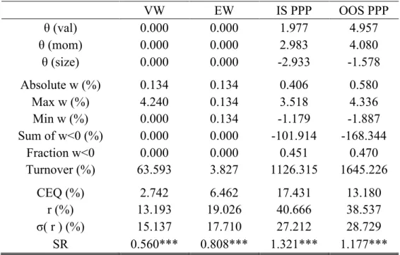
Table III – Base Case Portfolio Policy

The table shows the results of the optimization (Eq. 4) of a power utility function with a risk aversion of five with three characteristics: value (val), momentum (mom), and size. The four columns labeled “VW”, “EW”, “IS PPP”, and “OOS PPP” are representative of the results obtained in the value-weighted portfolio, equal-weighted portfolio, in-sample parametric portfolio policy, and out-of-sample parametric portfolio policy, respectively. The first three rows are the estimated coefficients for each characteristic. The out-of-sample coefficients are averaged across the time span. These statistics are followed by the average absolute portfolio weight, the average maximum weight, the average minimum weight, the average sum of negative positions, the average fraction of negative position in the overall portfolio, and, last, the portfolio turnover. This second set of statistics represents time-series averages of those monthly statistics. The final set of rows includes performance metrics: certainty equivalent return, average return, standard deviation of returns, and Sharpe ratio. For the out-of-sample calculations I compute the coefficients each year using the expanding window method. The coefficients are used for constructing out-of-sample portfolios for the twelve months that follow it. The *, **, and *** state the significance of the Sharpe ratio being above zero for 90%, 95%, and 99% significance level.

VW EW IS PPP OOS PPP θ (val) 0.000 0.000 1.977 4.957 θ (mom) 0.000 0.000 2.983 4.080 θ (size) 0.000 0.000 -2.933 -1.578 Absolute w (%) 0.134 0.134 0.406 0.580 Max w (%) 4.240 0.134 3.518 4.336 Min w (%) 0.000 0.134 -1.179 -1.887 Sum of w<0 (%) 0.000 0.000 -101.914 -168.344 Fraction w<0 0.000 0.000 0.451 0.470 Turnover (%) 63.593 3.827 1126.315 1645.226 CEQ (%) 2.742 6.462 17.431 13.180 r (%) 13.193 19.026 40.666 38.537 σ( r ) (%) 15.137 17.710 27.212 28.729 SR 0.560*** 0.808*** 1.321*** 1.177***

Although the investment universe being analyzed is of large stocks only, my findings are similar to those of Brandt, Santa-Clara and Valkanov (2009). This strategy has a particularity, the

weight allocated to each stock is a deviation from the weight that same stock has on the benchmark portfolio. The deviation depends on the characteristics of the stock and the coefficient loading for each of the characteristics.

Through the in-sample analysis (“IS PPP”) I found that the coefficients for value and momentum are positive while the size one is negative. This means that the parametric portfolio’s optimal weights deviate negatively with the firm’s size and positively with both the value and momentum of the firm. The coefficient with the highest loading is the momentum one, hence, a higher momentum triggers a larger overweight of a stock.

From the second set of rows in the table we can see that despite the strategy having an average absolute weight of approximately three times both the value-weighted and the equal-weighted portfolio, the maximum and minimum average weights for the parametric portfolio are 3.52% and -1.18%. Meaning the positions taken are not extreme and are possibly due to not having any restriction on short sales, while the value- and equal-weighted portfolio are long-only. The policy portfolio has an annual turnover of approximately 1126%, this level of turnover means the policy is hardly implementable if transaction costs are to be considered. This can have a large impact on performance. This value of turnover is extreme when compared to the benchmarks’ turnover of 63.6% and 3.8% for the value-weighted and equal-weighted portfolio, respectively, but the two benchmarks are not affected by changes in stock’s characteristics. The very low turnover in the equal-weighted portfolio is due to the stability of the sample of large stocks and is mostly affected by new listings, delistings, and equity issues, while the value-weighted portfolio only changes the allocation of wealth with the firms’ market capitalization, The third set of rows displays performance measures for the different asset allocation strategies, all the values are annualized. The optimal portfolio has a return of 40.67% and a standard deviation of returns of 27.21%. When comparing with the value-weighted portfolio it is possible to see that the return of the optimal strategy is approximately 308% of the benchmark while the standard deviation is only 180%, approximately, higher. This is reflected on the Sharpe ratio, a measure of the risk-return trade-off. The optimal portfolio reaches 1.32, an outstanding value when compared to 0.56 and 0.808, of the value- and equal-weighted portfolios, respectively. In terms of certainty equivalent returns this strategy also outperforms both the benchmarks, the equivalent risk-free rate needed for an investor to trade this strategy for a riskless outcome would be approximately 17.43% annualized return.

Based on the Opdyke (2007) I do a statistical test for the difference in Sharpe ratios, more precisely, H0: SRbase case ≥ SRbenchamark for both the value-weighted and equal weighted (naïve)

benchmarks. The Sharpe ratio of the base case (ɣ=5) is statistically larger than both the benchmarks at the 99% level (p-value is 0.9998 and 1.0000 for the naïve and value weighted portfolio). Implying this strategy brings a significant improve in the risk-return trade off an investor faces.

It must be noted that this analysis regards an in-sample optimization, hence, it is not unexpected that the strategy outperforms the benchmarks. I proceed to do an out-of-sample analysis to check the strategy’s robustness (as shown in the fourth column of Table III).

I do an estimation of the initial coefficients using 10 years of data, from December 1964 to November 1974, and use those coefficients to form monthly portfolios for the following 12 months. After, I re-estimate the coefficients with an expanding window, which is the enlargement of the sample, and construct the following year monthly portfolios with the new coefficients. This is done every year until the end of the sample.

In the out-of-sample results the signs of the coefficients remain the same, but it is possible to see a change in the coefficient loadings. Value and momentum have a higher impact on the deviations of the optimal portfolio weights from the benchmark, while size diminishes its influence. The principal change is in the fact that value is now the characteristic with the highest loading.

Concerning the allocations, the average absolute weight is higher, as also the average maximum and minimum weights are with values of 0.58%, 4.34%, and -1.89%, respectively. The allocations remain to not be extreme. The turnover increases to 1645% approximately, the magnitude of this measure is a relatively big concern for the practical implementation of the strategy. An important aspect of the out-of-sample portfolios is the performance measures which did not have a large decline. The average return is 38.54%, only 2p.p. lower than the one of the in-sample portfolios. The volatility increased by approximately 1.5p.p.. This leads to a lower Sharpe ratio of 1.18.

Figure II – Cumulative portfolio returns

The figure displays the cumulative portfolio return over the investment period from January 1975 to December 2015 of the in-sample optimal portfolio, out-of-sample optimal portfolio, naïve portfolio, and value-weighted portfolio.

The optimal portfolio policy provides for larger cumulative returns. There is not a meaningful out-of-sample deterioration in this metric, both lines follow closely. One thing must be noted, the ‘movements’ of the portfolio policy follow the ones of the naïve and value-weighted portfolio. Therefore, this strategy follows the market trends and, hence, should not be used as hedging strategy against market risk. Due to the high exposure to the market it is possible to see more accentuated drops than in the both the benchmarks, but the increases are also higher. The the optimal portfolio allows for short selling which is the cause for the increased exposure. The use of the three characteristics value, size, and momentum must be pointed out has one of the factors to why there is not a large deterioration in the out-of-sample results. These characteristics are stable through time and previously known to be related to sizeable risk-adjusted returns.

There are different factors that may have affected these results in a negative way. First, despite rebalancing the weights monthly, the coefficients are only calculated once every twelve months. Increasing the frequency at which coefficients are recalculated can be a way to improve performance. Second, enlarging the sample to include small and mid size stocks can lead to a lower turnover. An event that affects mostly large stocks can have a significant impact in the stocks’ characteristics (eg. momentum) and lead to an increase in trading activity, and, therefore, turnover. 0 200 400 600 800 1000 1200 1400 1600 1800 2000 Ja n-75 Jun -76 N ov -77 A pr -79 Se p-80 Fe b-82 Jul -83 De c-84 Ma y-86 Oc t-87 Ma r-89 A ug -90 Ja n-92 Jun -93 N ov -94 A pr -96 Se p-97 Fe b-99 Jul -00 De c-01 Ma y-03 Oc t-04 Ma r-06 A ug -07 Ja n-09 Jun -10 N ov -11 A pr -13 Se p-14 IS OOS Naive VW

b. Unconstrained Optimization with Five Characteristics

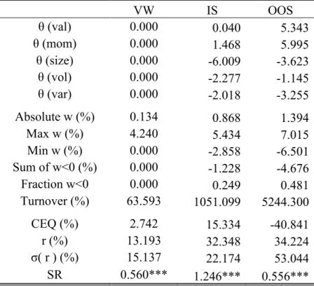
Table IV – Portfolio Policy with Five Characteristics

The table display the optimization results of a power utility function with a risk aversion of five and using five characteristics: value (val), momentum (mom), size, volatility (vol), and tail risk (tail). Characteristics are standardized cross-sectionally. The three columns labeled “VW”, “IS”, and “OOS” are representative of the results obtained in the value-weighted portfolio, in-sample optimal portfolio, and out-of-in-sample optimal portfolios, respectively. The five first rows are the estimated coefficients for each characteristic, the out-of-sample coefficients are averaged throughout the time span. These statistics are followed by the average absolute portfolio weight, the average maximum weight, the average minimum weight, the average sum of negative positions, the average fraction of negative position in the overall portfolio, and, last, the portfolio turnover. The turnover measure is annualized. This second set of statistics represents time-series averages of those monthly statistics. The final set of rows includes performance metrics: certainty equivalent return, average return, standard deviation of returns, and Sharpe ratio. For the out-of-sample calculations I compute the coefficients each year using the expanding window method. The coefficients are used for constructing out-of-sample portfolios for the twelve months that follow it. The *, **, and *** state the significance of the Sharpe ratio being above zero for 90%, 95%, and 99% significance level.

VW IS OOS θ (val) 0.000 0.040 5.343 θ (mom) 0.000 1.468 5.995 θ (size) 0.000 -6.009 -3.623 θ (vol) 0.000 -2.277 -1.145 θ (var) 0.000 -2.018 -3.255 Absolute w (%) 0.134 0.868 1.394 Max w (%) 4.240 5.434 7.015 Min w (%) 0.000 -2.858 -6.501 Sum of w<0 (%) 0.000 -1.228 -4.676 Fraction w<0 0.000 0.249 0.481 Turnover (%) 63.593 1051.099 5244.300 CEQ (%) 2.742 15.334 -40.841 r (%) 13.193 32.348 34.224 σ( r ) (%) 15.137 22.174 53.044 SR 0.560*** 1.246*** 0.556***

The three characteristics exploited by the base case – value, size, and momentum - have long been known in the literature to be related with above average risk-adjusted returns. Furthermore, those characteristics have been shown to be persistent throughout time.

By adding two characteristics – volatility and tail risk - that are not so deeply exploited by the literature my aim is to see how the model behaves. Below I show a table with the results from this policy and compare it with the value-weighted market portfolio.

In the in-sample analysis it is possible to observe that the coefficients for value, momentum, and size continue to have the same signal. The two first are positive, while size has a negative sign. The two characteristics introduced – volatility and tail risk – have negative coefficients. This means that, together with size, they trigger negative deviations from the weights in the valueweighted portfolio benchmark. The magnitude of the size coefficient is the largest, -6.009, followed by volatility and tail risk with -2.277 and -2.018, respectively.

Regarding portfolio allocations this policy has more extreme allocations. The average absolute weight is 0.868%. In comparison with the other strategies, is approximately six and a half and two and a half times the average absolute weight of the benchmark and the base case, respectively. The average sum of negative positions is -122.8%, this means that the positive weights sum 222.8%, which is quite extreme. There is a marginal improvement in turnover, nevertheless, this measure remains too large to be feasible and easily implemented in real world markets.

The certainty equivalent return deteriorated to 15.33% in comparison with the base case. The decrease in Sharpe ratio is approximately 0.08. With a confidence level of 99% the Sharpe ratio is significantly positive. As in the base case I do a test for Ho: SR5char ≥ SRbenchmark. Although I

only display the statistics for the value-weighted portfolio on Table IV I do the test for both the naïve and the value-weighted portfolios, using the same test by Opdyke (2007). With 99% significance I can infer that the Sharpe ratio of the policy portfolio with five characteristics is higher than the one of both the benchmarks (p-value is 0.9946 and 0.9999 for the naïve and value-weighted benchmark, respectively).

For robustness, I also do an out-of-sample analysis of this portfolio policy. Although the signs of the coefficients remain the same their magnitudes change. Value and momentum have the highest coefficient loadings of 5.343 and 5.995, respectively. Size and volatility decrease their

Concerning the portfolio weights the allocation is more extreme than in the in-sample portfolio. The average absolute weight is 1.394%, more than ten times the one of the benchmark. The average sum of negative weights is -467.6%, meaning there are 567.6% positive allocations. Also, turnover is more than five times larger than its in-sample counterpart.

Regarding performance analysis, the return only increases approximately 2p.p. for twice the volatility. This means that the risk-return trade off represented by the Sharpe ratio falls to below half of what was its in-sample value, 0.556. I test the H0: SRIS ≥ SROOS and with 95% confidence

level the null hypothesis is not rejected (p-value of 0.9983). Hence, there is significant deterioration in performance when implementing this strategy.

The deterioration of performance when conducting out-of-sample analysis should be the main concern for an investor that tries to expand the number of characteristics in the model. Even when ignoring the need for a margin account the five characteristic portfolio policy is extreme and its performance deteriorates when conducting out-of-sample performance analysis. Both the characteristics introduced are not as persistent as the ones from the base case, which can be one reason for the large performance decrease. Second, volatility and tail risk are related to whether the market is bull or bear, which can change several times during a short period of time leading to more variability in the results.

An investor that wants to expand this model to include more information on stocks should choose characteristics that are known to be persistent and have been previously known to be linked to above average risk adjusted returns. This can be considered a snooping bias, but as it was proven in the analysis above, adding random characteristics does not bring robust benefits on performance. The approach of trying to include more characteristics as if an investors did not know beforehand which ones brought more favorable risk adjusted returns such as Lewellen (2014) does by expanding the models to better forecast expected stock returns and construct portfolios from those, does not work in the model by Brandt, Santa-Clara and Valkanov (2009) as they model directly the weights and do no do forecasts before. Furthermore, despite just being a short extension it increases the computations in the model. In an extreme, if one tries to include all information regarding stocks in the model it would eventually become computationally exhausting.

c. Portfolio Policy with Industry Standardization

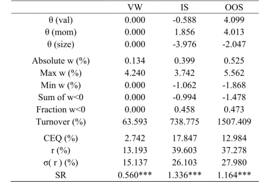
Table V – Portfolio Policy with Industry Standardization

The table shows the results of the optimization (eq. 4) of a power utility function with a risk aversion of five with three characteristics: value (val), momentum (mom), and size. In this case the cross-sectional standardization of characteristics is done using the mean and standard deviation of each stock’s division. The three columns labeled “VW”, “IS”, and “OOS” are representative of the results obtained in the value-weighted portfolio, in-sample optimal portfolio, and out-of-sample optimal portfolios, respectively. The first three rows are the estimated coefficients for each characteristic. The out-of-sample coefficients are averaged across the time span. These statistics are followed by the average absolute portfolio weight, the average maximum and minimum weight, the average sum of negative positions, the average fraction of negative position in the overall portfolio, and, last, the portfolio turnover. This second set of statistics represents time-series averages of those monthly statistics. The final set of rows includes performance metrics: certainty equivalent return, average return, standard deviation of returns, and Sharpe ratio. For the out-of-sample calculations I compute the coefficients each year using the expanding window method. The coefficients are used for constructing out-of-sample portfolios for the twelve months that follow it. The *, **, and *** state the significance of the Sharpe ratio being above zero for 90%, 95%, and 99% significance level. VW IS OOS θ (val) 0.000 -0.588 4.099 θ (mom) 0.000 1.856 4.013 θ (size) 0.000 -3.976 -2.047 Absolute w (%) 0.134 0.399 0.525 Max w (%) 4.240 3.742 5.562 Min w (%) 0.000 -1.062 -1.868 Sum of w<0 0.000 -0.994 -1.478 Fraction w<0 0.000 0.458 0.473 Turnover (%) 63.593 738.775 1507.409 CEQ (%) 2.742 17.847 12.984 r (%) 13.193 39.603 37.278 σ( r ) (%) 15.137 26.103 27.980 SR 0.560*** 1.336*** 1.164***

As it is possible to see from the table above the coefficients follow the same trend as in the unconstrained policy with the exception of value, that presents a negative in-sample coefficient. In the in-sample analysis momentum plays the most important role in setting the deviations from the benchmark weights. The weights remain fairly stable, there are no extreme allocations to stocks, which increases the feasibility of the strategy. There is a marginal improvement in the fraction of negative positions when comparing with the base case (0.384 vs. 0.381). The improvement in turnover has to be highlighted. This measure decreases to approximately 739% while performance suffers a marginal improvement.

Using the Opdyke (2007) statistical test for the significance of Sharpe ratios I can infer with 99% confidence that the null hypothesis, H0: SRind ≥ SRbenchmark, cannot be rejected. Meaning,

with 99% significance using industry standardization when constructing portfolios provides a higher risk-return trade off than investing on a portfolio that mimics the benchmarks, both the and equal-weighted portfolio (p-value of 0.9999 and 1.0000 for the naïve and value-weighted portfolio).

In terms of performance there is a slight increase in the certainty equivalent measure to 17.85%. The Sharpe ratio is 0.015 higher, therefore I test the hypothesis SRindustry=SRbase case. I conclude

that the difference in Sharpe ratios is not significant at a 95% confidence level (p-values equals 0.9159). Hence, the increase in Sharpe ratio is not a reliable framework for defining it as a better strategy than the base case.

When proceeding for the out-of-sample analysis to assess the robustness of this strategy I find that value plays the most important role, alongside momentum. Both characteristics’ coefficients enlarge out-of-sample while the one for size decreases in absolute terms.

There is a large increase in turnover from the in-sample analysis to the out-of-sample. Despite the large increase it still performs better than the out-of-sample base case. The certainty equivalent is 12.98%. One thing must be noted, there is not a large deterioration in Sharpe ratio when moving to the out-of-sample analysis. The Sharpe measure is 1.164 compared to the 1.336 in-sample.

The standardization of characteristics to include differences in divisions can be beneficial for an investor. There are possibilities to try to take more advantage of this improvement. One can be to deepen the segregation and use the full SIC Code to allocate stocks. Second, if the different accounting practices across divisions are well known there is the possibility of creating adjustment factors for those and use them to standardize the cross-sectional characteristics. This

way, even though the standardization would be with the full cross-section all those accounting differences would already be accounted for.

d. Constrained Optimization

Table VI – Portfolio Policy with No Short-Sales

The table display the optimization results of a power utility function with a risk aversion of five and using three characteristics: value (val), momentum (mom), and size. Characteristics are standardized in the cross-section. I constrain the model to only allow for positive weights as explained in equation (5). The three columns labeled “VW”, “IS”, and “OOS” are representative of the results obtained in the value-weighted portfolio, in-sample optimal portfolio, and out-of-sample optimal portfolios, respectively. The three first rows are the estimated coefficients for each characteristic, the out-of-sample coefficients are averaged throughout the time span. These statistics are followed by the average absolute portfolio weight, the average maximum and minimum weight, the average sum of negative positions, the average fraction of negative position in the overall portfolio, and, last, the annual portfolio turnover. This second set represents time-series averages of the monthly statistics. The final set of rows includes performance metrics: certainty equivalent return, average return, standard deviation of returns, and Sharpe ratio. For the out-of-sample calculations I compute the coefficients each year using the expanding window method. The coefficients are used for constructing out-of-sample portfolios for the twelve months that follow it. The *, **, and *** state the significance of the Sharpe ratio being above zero for 90%, 95%, and 99% significance level.

VW IS OOS θ (val) 0.000 -1.730 4.957 θ (mom) 0.000 3.556 4.080 θ (size) 0.000 -5.555 -1.578 Absolute w (%) 0.134 0.282 0.288 Max w (%) 4.240 1.326 1.394 Min w (%) 0.000 0.001 0.001 Sum w<0 (%) 0.000 0.000 0.000 Fraction w<0 0.000 0.000 0.000 Turnover (%) 63.593 243.952 311.705 CEQ (%) 2.742 0.131 12.194

Some practitioners face everyday one of the most common investment restriction, they are not allowed to make short sales. Hence, they can only take advantage of positive news while leaving out the possibility of extra returns from negative news. Furthermore, an unconstrained investor can increase the exposure to the benefits brought by long positions through the proceeds from short selling. I include this restriction in my analysis with the aim of intertwining this strategy with the investors’ needs.

There is a change in the coefficients from the unconstrained portfolio policies examined before. Considering the in-sample (IS) performance, in this constrained case the coefficient for value changes sign and is now negative. Meaning, value firms are no longer preferred, just like large firms. The largest coefficient in absolute terms is size, therefore, the larger the firm the higher the deviation from the benchmark portfolio is.

Although the wealth allocation to each stock in the previous cases is not extreme, the constrained case figures are even lower. The average maximum and minimum weight allocated to a stock is 1.33% and 0.00%, respectively. The average weight is 0.28%.

The most noticeable improvement that constraining the weights brings is in terms of turnover. The turnover reduction is approximately 882%, from 1085% (column 3, Table III) to 244%. The turnover is in annual terms. Although this figure is still high, it represents a large improvement from the base case and a more feasible implementation.

Performance measures are displayed on the third set of rows. The optimal constrained portfolio has an annualized return of 29.14% and a standard deviation of returns of 21.32%. In terms of Sharpe ratio there is a decrease to 1.145.

The long-only policy portfolio is the one that most resembles the benchmarks. By not being able to take advantage of the negative forecasts it loses the opportunity to make extra returns from it. Therefore, statistically comparing the risk-return trade off, Sharpe ratio, performance between this policy portfolio and the benchmarks is crucial for the analysis. I test the following null hypothesis, H0: SRconstraines ≥ SRbenchmark. As in the other cases I use the Opdyke (2007) test.

Despite being a long-only strategy, it still performs well in the statistical tests. At a 99% confidence level, the null hypothesis holds and, therefore, this strategy outperforms both the benchmarks (naïve and value-weighted) in terms of Sharpe ratio (p-value of 1.0000 and 0.9982 for the value- and equal-weighted portfolio).

When checking for out-of-sample robustness I use the same methodology as in the base case. The sign of the value coefficient changes and its absolute value is higher than in the in-sample

analysis. According to this analysis, an investor prefers value firms to growth firms. Value becomes the coefficient that most deviation brings from the original benchmark weights. Although the average weight is higher than the one in the in-sample portfolios, the increase of 0.006p.p. does not raise concerns in terms of extreme out-of-sample allocations. There is a rise of 67.75 p.p. in turnover.

Figure III – Cumulative returns for long-only policy portfolio

The figure displays the cumulative portfolio return over the investment period from January 1975 to December 2015 of the in-sample optimal portfolio, out-of-sample optimal portfolio, naïve portfolio, and value-weighted portfolio, for a long-only policy portfolio.

The benefits of employing a Brandt, Santa-Clara, and Valkanov (2009) long-only portfolio optimization leads to improvements in terms of out-of-sample variability in results. The decrease in Sharpe ratio is only marginal and there is not a large deterioration in certainty equivalent. Overall when choosing whether to implement this strategy or the base case an investor should evaluate the trade-off between a small deterioration in Sharpe ratio and a large turnover. 0 200 400 600 800 1000 1200 1400 De c-74 Ju l-76 Fe b-78 Se p-79 Ap r-81 No v-82 Ju n-84 Ja n-86 Au g-87 Ma r-89 Oc t-90 Ma y-92 De c-93 Ju l-95 Fe b-97 Se p-98 Ap r-00 No v-01 Ju n-03 Ja n-05 Au g-06 Ma r-08 Oc t-09 Ma y-11 De c-12 Ju l-14 IS OOS Naive VW

e. Varying risk aversion

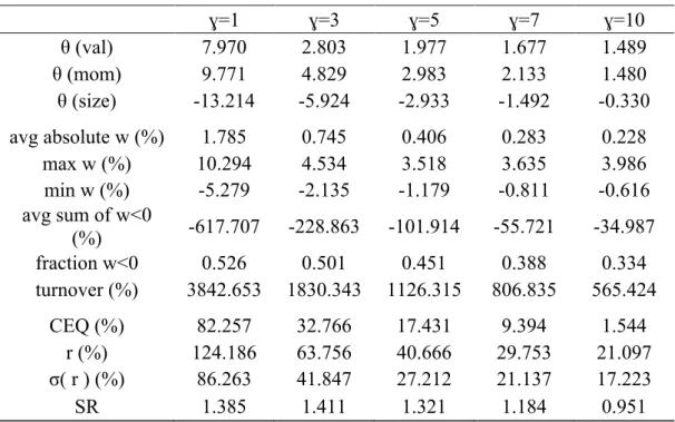
Table VII – Portfolio Policy with Varying Risk Aversion

The table shows the results of the portfolio optimization (Eq. 4) with three characteristics: value (val), momentum (mom), and size. The optimization is done with different power utility functions with relative risk aversion of one, three, five (base case), seven, and ten. Panel A and Panel B display in-sample and out-of-sample results, respectively. The three first rows are the estimated coefficients for each characteristic, the out-of-sample coefficients are averaged throughout time. Followed by the average absolute portfolio weight, the average maximum weight, the average minimum weight, the average sum of negative positions, the average fraction of negative position, and the portfolio annual turnover. This second set of statistics represents time-series averages of those monthly statistics. The final set of rows includes performance metrics: certainty equivalent return, average return, standard deviation of returns, and Sharpe ratio. For the out-of-sample calculations I compute the coefficients each year using the expanding window method. The coefficients are used for constructing out-of-sample portfolios for the twelve months that follow it. The *, **, and *** state the significance of the Sharpe ratio being above zero for 90%, 95%, and 99% significance level.

Panel A. In-sample optimization

ɣ=1 ɣ=3 ɣ=5 ɣ=7 ɣ=10 θ (val) 7.970 2.803 1.977 1.677 1.489 θ (mom) 9.771 4.829 2.983 2.133 1.480 θ (size) -13.214 -5.924 -2.933 -1.492 -0.330 avg absolute w (%) 1.785 0.745 0.406 0.283 0.228 max w (%) 10.294 4.534 3.518 3.635 3.986 min w (%) -5.279 -2.135 -1.179 -0.811 -0.616 avg sum of w<0 (%) -617.707 -228.863 -101.914 -55.721 -34.987 fraction w<0 0.526 0.501 0.451 0.388 0.334 turnover (%) 3842.653 1830.343 1126.315 806.835 565.424 CEQ (%) 82.257 32.766 17.431 9.394 1.544 r (%) 124.186 63.756 40.666 29.753 21.097 σ( r ) (%) 86.263 41.847 27.212 21.137 17.223 SR 1.385 1.411 1.321 1.184 0.951

Panel B. Out-of-sample optimization ɣ=1 ɣ=3 ɣ=5 ɣ=7 ɣ=10 θ (val) 16.180 6.943 4.957 4.121 3.518 θ (mom) 14.228 6.569 4.080 2.930 2.032 θ (size) -9.092 -3.633 -1.578 -0.605 0.168 avg absolute w (%) 2.185 0.919 0.580 0.449 0.373 max w (%) 14.215 6.109 4.336 3.902 3.936 min w (%) -6.896 -2.960 -1.887 -1.457 -1.177 avg sum of w<0 (%) -7.703 -2.952 -168.344 -1.196 -0.908 fraction w<0 0.530 0.501 0.470 0.446 0.427 turnover (%) 5792.775 2623.714 1645.226 1199.950 858.739 CEQ (%) 71.607 26.551 13.180 5.947 -1.416 r (%) 119.456 59.092 38.537 28.962 21.442 σ( r ) (%) 92.873 43.064 28.729 22.862 19.045 SR 1.235 1.263 1.177 1.060 0.878

All the portfolio policies presented before assume that the investor’s risk aversion can be translated to a coefficient equal to five. When modelling the utility function, the risk aversion coefficient plays a big role in allocating wealth throughout the available assets. My aim here is to assess how changing this assumption affects the portfolio outcome, both in terms of coefficients and performance metrics.

The signs of the coefficients remain the same throughout all levels of risk aversion. Hence, independently of risk preferences, an investor prefers smaller firms, past winners, and value firms. The absolute value of the coefficients decreases with the increase in the level of risk aversion, suggesting the three characteristics are related to mean returns and risk. This means that the less the risk aversion the more the weights will deviate from the benchmark weights, leading to more extreme allocations. This can be seen in the second set of rows of the table (Table VII) in both panels.

An investor with ɣ=1 – low risk aversion – incurs on more short positions, the size of such positions is also larger. When compared to the base case (ɣ=5), the fraction of negative weights in the portfolio is only 7.5% larger, implying the bets on stocks are similar, but the decrease in risk aversion indicates the use of more leverage. An investor with ɣ=1 has -617.7% of negative

a 3843% annual turnover approximately. On the other hand, when ɣ=10 – high risk aversion – the investor holds approximately 135% long positions, and the turnover figure is 565% annual, half of what the base case provides. Despite looking as a more attractive strategy for an investor that wants to avoid risk taking in terms of turnover and asset allocation, the certainty equivalent (CEQ) when ɣ=10 is negative, meaning the investor is better off leaving this strategy behind and investing in the riskless asset.

Both in-sample (IS) and out-of-sample (OOS), from ɣ=2 to ɣ=10, there are increases in Sharpe ratio with the decrease of risk aversion. Implying the investor receives more return per unit of risk bore. Nevertheless, when ɣ=1 there is a marginal decrease in Sharpe ratio. At such an extreme level of risk the return received per unit of risk taken decreases.

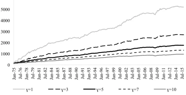
Figure IV – Cumulative return of varying risk aversion

The figure displays the in-sample cumulative returns for portfolios constructed according to different power utility functions with relative risk aversion of one, three, five (as in the previous analysis), seven, and ten over the investment period from January 1975 to December 2015.

This figure shows what has been mentioned before, the lower the risk aversion the larger the investor’s bets. The higher return is also due to the short positions providing some hedge on the stocks that perform worse.

f. Lewellen (2014) Strategy 0 1000 2000 3000 4000 5000 6000 Ja n-75 Jul -76 Ja n-78 Jul -79 Ja n-81 Jul -82 Ja n-84 Jul -85 Ja n-87 Jul -88 Ja n-90 Jul -91 Ja n-93 Jul -94 Ja n-96 Jul -97 Ja n-99 Jul -00 Ja n-02 Jul -03 Ja n-05 Jul -06 Ja n-08 Jul -09 Ja n-11 Jul -12 Ja n-14 Jul -15 ɣ=1 ɣ=3 ɣ=5 ɣ=7 ɣ=10

My focus here is not on proving how reliable estimates of expected returns provided by model one in Lewellen (2014) are. My aim is to compare it with the long only portfolio by Brandt, Santa-Clara and Valkanov (2009).

In this section I use the strategy constructed by Lewellen (2014) to form long-only monthly portfolios of stocks. I allocate wealth to the stocks that are above the 50th percentile. I use FM regressions to estimate the expected return of each stock. As in the other strategies employed I only consider firms that have all the characteristics available at the time.

Lewellen (2014) chooses as a threshold for the long policy the 90th percentile of stocks. This is not logical as I am only assessing the behavior of the S&P500. Using only the 90th percentile to invest in would not be appropriate due to the size of my sample.

I construct two portfolios of stocks. One goes long on the 75th percentile. The second portfolio resembles the first one but goes long on the 50th percentile. Due to the number of stocks in my sample investing in long positions on the 90th percentile only as Lewellen (2014) does would not be appropriate since the average number of stocks included may not be sufficient to extract enough diversification benefits. Enlarging the percentiles tackles this loss and allows to make a more informed comparison without incurring in a small sample bias.

According to the forecasted expected returns I equal-weight my investment across the stocks that meet the percentile requirements and, hence, are included in the portfolio.

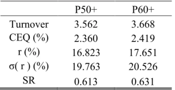
Table VIII – Portfolio Statistics

The table below reports the turnover, certainty equivalent return (CEQ), return, standard deviation, and Sharpe ratio for a portfolio of stocks that meet the 50th _{percentile threshold in}

the estimated expected returns (P50+) and a portfolio of stocks that meet the 60th percentile threshold (P60+). All values are annualized. For the certainty equivalent return computations, I assume a risk aversion coefficient of five.

P50+ P60+ Turnover 3.562 3.668 CEQ (%) 2.360 2.419 r (%) 16.823 17.651 σ( r ) (%) 19.763 20.526 SR _{0.613 0.631}

Since these portfolios are equally weighted the low turnover figure is not surprising. Turnover is only affected by new listings and delistings, that cause the sample to enlarge or diminish, or if firms that meet the percentile requirements change. The turnover resembles the one of the equal-weighted portfolio presented in Table III. In comparison with the turnover provided by the other strategies exploited in this thesis this one is by far the best value. Nevertheless, the remaining statistics fail to meet their counterparts from the naïve portfolio (column 2, Table III).

Overall, it is best to equally allocate wealth to firms in the whole universe of stocks than to sort them into percentiles and define a threshold.

IV. Conclusion

I test the Brandt, Santa-Clara, and Valkanov (2009) approach for a portfolio of large stocks only. My aim is to asses whether their argument that it is ‘easily modified and extended’ holds when introducing three different cases to their base case. The base case models the weights allocated to each stock according to three characteristics: value, size, and momentum. I extend the characteristics used to incorporate volatility and tail risk. I also use characteristics standardization within the divisions provided by the SIC Code to find optimal portfolios. Finally, I model the constrained case to allow investors with short selling limitations to use this model.

In the base case and the model with five characteristics there is more wealth allocated to small firms, value firms, and past winners. In the extended model firms that are less volatile and firms with less tail risk are favorites. All these strategies have large certainty equivalent returns and significant Sharpe ratios at the 99% confidence level. What makes them less likely to be implemented by fund managers is the high turnover.

Standardizing the characteristics by industry specific means and standard deviations has similar results as the long-only case. Both allocate more wealth to small firms and past winners, but now growth firms are preferred over value firms. There is not a large deterioration in results when comparing to the base case in terms of certainty equivalent and Sharpe ratio. Both models in-sample provide more attractive values for turnover, easing the implementation process. The long-only portfolio turnover holds through robustness tests, making it the most attractive strategy when using the Brandt, Santa-Clara, and Valkanov (2009) approach.

The results given by the Lewellen (2014) specification fail to meet the equally-weighted in terms of performance. Hence, this strategy main focus should be in forecasting returns and not on constructing portfolios from it.

References

Asness, Clifford S., R. Burt Porter, and Ross L. Stevens, 2001, “Predicting Stock Returns Using Industry-Relative Firm Characteristics”, Working Paper, AQR Capital Management

Brandt, Michael W. and Pedro Santa-Clara, 2006, “Dynamic Portfolio Selection by Augmenting the Asset Space”, Journal of Finance 61:2187-217

Brandt, Michael W., Pedro Santa-Clara and Rossen Valkanov, 2009, “Parametric Portfolio Policies: Exploiting Characteristics in the Cross-Section of Equity Returns”, Review of

Financial Studies, 22(9)

Brandt, Michael W., 2010, “Portfolio Choice Problems”, Handbook of Financial Econometrics Chan, Louis K.C., Jason Karceski and Josef Lakonishok, 1998, “The Risk and Return from Factors”, Journal of Financial and Quantitative Analysis 33:159-88

DeMiguel, Victor, Lorenzo Garlappi and Raman Uppal, 2007, “Optimal versus Naïve Diversification: How Inefficient is the 1/N Portfolio Strategy”, Review of Financial Studies, 0 Fama, Eugene F., Kenneth R. French, 1992, “The cross-section of expected stock returns”,

Journal of Finance 47:427-465

Fama, Eugene F., Kenneth R. French, 1996, “Multifactor Explanations of Asset Pricing Anomalies”, Journal of Finance 51:55-84

Fama, Eugene F., James MacBeth, 1973, “Risk, return and equilibrium: Empirical tests”,

Journal of Political Economy 81:607-636

Hanna, J. Douglas, Mark Ready, 2005, “Profitable predictability in the cross section of stock returns”, Journal of Financial Economics 78:463-505

Lewellen, Jonathan, 2014, “The Cross Section of Expected Stock Returns”, Working Paper, Dartmouth College.

Markowitz, Harry, 1952, “Portfolio Selection”, Journal of Finance 7, 77-91

Opdyke, J.D., 2007. “Comparing Sharpe ratios: so where are the p-values?” Journal of Asset

Management 8 (5), 308–336

Pástor, Lubos, and Pietro Veronesi, 2009, “Learning in Financial Markets,” Annual Review of