Fundação Getúlio Vargas
Essays on Regulation and Risk
Tese submetida à Escola de Pós-Graduação em Economia da Fundação Getúlio Vargas como requisito de obtenção do
título de Doutor em Economia
Aluno: Régio Soares Ferreira Martins
Orientador: Humberto Luiz Ataíde Moreira
Escola de Pós-Graduação em Economia - EPGE
Fundação Getúlio Vargas
Essays on Regulation and Risk
Tese submetida à Escola de Pós-Graduação em Economia da Fundação Getúlio Vargas como requisito de obtenção do
título de Doutor em Economia
Aluno: Régio Soares Ferreira Martins
Banca Examinadora:
Humberto Luiz Ataíde Moreira (Orientador, EPGE-FGV)
Renato Galvão Flôres Junior (EPGE/FGV)
Caio Ibsen Rodrigues de Almeida (EPGE/FGV)
Vinícius Carrasco (PUC/RJ)
Rodrigo de Losso da Silveira Bueno (FEA/USP)
Agradeço,
Ao Humberto, pelas discussões, preocupações e cobranças que foram funda-mentais para a conclusão desse trabalho.
Aos membros da banca examinadora, pela paciência na leitura dos artigos, sugestões e constribuições feitas.
Ao meu co-autor, Daniel Lima, pelas ideias, discussões (e diversões) em San Diego.
RESUMO
Essa tese investiga alguns aspectos da relação entre regulação econômica e risco da empresa regulada. No primeiro capítulo, o objetivo é entender as implicações do modelo tradicional de regulação por incentivos (Laffont e Tirole, 1993) sobre o risco sistemático da firma. Generalizamos o modelo de forma a incorporar risco agregado ao lucro da atividade, e descobrimos que o contrato ótimo deve ser severamente restringido para que reproduza betas (CAPM) próximos aos observados em setores regulados. Usamos um caso particular do modelo, de regulação por repartição de lucro (profit-sharing regulation), para avaliar a relação entre a potência do contrato e o nível de risco não diversificável. Encontramos resultados compatíveis com a evidência disponível, de que regimes com alta potência impõem mais risco sobre a firma. No segundo capítulo, escrito em co-autoria com Daniel Lima da Uni-versidade da Califórnia em San Diego (UCSD), partimos da constatação de que empresas reguladas podem estar sujeitas a práticas regulatórias que po-tencialmente afetam a simetria da distribuição de seus lucros futuros. Se essas práticas forem antecipadas pelos investidores no mercado secundário de ações, poderemos identificar diferenças no padrão da assimetria da dis-tribuição empírica de retornos das empresas reguladas com relação às não-reguladas. Nesse capítulo revisamos alguns métodos de mensuração de as-simetria propostos recentemente na literatura, que são robustos à caracterís-ticas comuns em séries de retornos financeiros (caudas pesadas e correlação serial), e investigamos se existem diferenças significativas na distribuição de assimetria entre empresas reguladas e não-reguladas.
No terceiro e último capítulo, três diferentes abordagens empíricas do modelo de apreçamento de ativos de Kraus e Litzenberger (1976) são testadas com dados do mercado brasileiro de ações. Descobrimos que a distribuição empírica de retornos costuma exibir co-assimetria significativa com relação à carteira de mercado, e que portanto os retornos das ações são sensíveis à volatilidade (retornos quadráticos) do mercado. No entanto, apesar da base teórica para a preferência por retornos assimétricos esteja bem estabelecida e seja bastante intuitiva, não encontramos evidência que suporte a hipótese de que os investidores requeiram um prêmio para aceitar esse tipo de risco no mercado local.
ABSTRACT
In this thesis, we investigate some aspects of the interplay between eco-nomic regulation and the risk of the regulated firm. In the first chapter, the main goal is to understand the implications a mainstream regulatory model (Laffont and Tirole, 1993) have on the systematic risk of the firm. We generalize the model in order to incorporate aggregate risk, and find that the optimal regulatory contract must be severely constrained in order to reproduce real-world systematic risk levels. We also consider the optimal profit-sharing mechanism, with an endogenous sharing rate, to explore the relationship between contract power and beta. We find results compatible with the available evidence that high-powered regimes impose more risk to the firm.
In the second chapter, a joint work with Daniel Lima from the University of California, San Diego (UCSD), we start from the observation that regu-lated firms are subject to some regulatory practices that potentially affect the symmetry of the distribution of their future profits. If these practices are anticipated by investors in the stock market, the pattern of asymmetry in the empirical distribution of stock returns may differ among regulated and non-regulated companies. We review some recently proposed asymme-try measures that are robust to the empirical regularities of return data and use them to investigate whether there are meaningful differences in the dis-tribution of asymmetry between these two groups of companies.
In the third and last chapter, three different approaches to the capital asset pricing model of Kraus and Litzenberger (1976) are tested with re-cent Brazilian data and estimated using the generalized method of moments (GMM) as a unifying procedure. We find that ex-post stock returns gener-ally exhibit statisticgener-ally significant coskewness with the market portfolio, and hence are sensitive to squared market returns. However, while the theoretical ground for the preference for skewness is well established and fairly intuitive, we did not find supporting evidence that investors require a premium for supporting this risk factor in Brazil.
1 Incentive Regulation and Beta 1
1.1 Introduction . . . 2
1.2 Model . . . 4
1.3 Regulatory Policies . . . 7
1.3.1 Complete Information (FB) . . . 7
1.3.2 Asymmetric Information . . . 10
1.4 Numerical Analysis . . . 18
1.4.1 Sensitivity ofβ to Industry Parameters . . . 21
1.4.2 Sensitivity ofβ to the Contract Space . . . 25
1.4.3 Sensitivity ofβ to Contract Power . . . 28
1.5 Conclusions . . . 31
2 Regulation and Return Asymmetry 33 2.1 Introduction . . . 34
2.2 Measuring Asymmetry in Financial Returns . . . 38
2.2.1 Unconditional Asymmetry Tests . . . 43
2.2.2 Conditional Asymmetry Tests . . . 45
2.2.3 Empirical Results of Asymmetry Tests . . . 46
2.3 Regulatory Status and Return Asymmetry . . . 47
2.3.1 Contingency Tables . . . 47
2.3.2 Equality of the Conditional Densities . . . 50
2.3.3 Location and Scale Differences . . . 52
2.4 Conclusions . . . 53
3 The Pricing of Coskewness Risk 55 3.1 Introduction . . . 56
3.2 Skewness in Asset Pricing . . . 60
3.2.1 A Fully Specified Equilibrium Model . . . 61
3.2.2 Arbitrage Pricing . . . 62
3.2.3 Stochastic Discount Factor . . . 64
3.3 Empirical Results . . . 65
3.3.1 Summary Statistics of Returns . . . 65
3.3.2 Estimates of the Three-Moment CAPM . . . 66
3.4 Conclusion . . . 67
A Appendix for Chapter 1 71 A.1 Regulation under Complete Information . . . 73
A.1.1 Optimal Payment Profile . . . 73
A.1.2 Optimal Investment . . . 73
A.2 Regulation under Asymmetric Information . . . 74
A.2.1 Cost Unobservability . . . 75
A.2.2 Price-Cap Regulation . . . 75
B Appendix for Chapter 2 77 B.1 Moments of the Return Process . . . 77
B.2 The Skewed-t Distribution . . . 79
B.3 Summary of Results . . . 80
C Appendix for Chapter 3 93 C.1 Descriptive Statistics of Return Data . . . 93
C.2 Estimation Results . . . 97
A.1 Average betas of regulated industries (global). . . 71 A.2 Historical returns of the U.S. equity market and risk-free rate. 72 A.3 Feasible parameter domain by the source of restriction. . . 72
B.1 Firms with significant skewness by the (2.9) and (2.11) tests. . 80 B.2 Results of the asymmetry tests described in Section 2.2.1, at
5% nominal size . . . 81 B.3 Results of the asymmetry tests described in Section 2.2.1, at
10% nominal size . . . 82 B.4 Results of the asymmetry tests described in Section 2.2.2, at
5% and 10% nominal sizes . . . 83 B.5 True contingency table under observability of S . . . 84 B.6 Observed tabulation based on an estimator Sbof S . . . 84 B.7 Odds ratio by period and asymmetry test performed. Power
= 95% . . . 85 B.8 Odds ratio by period and asymmetry test performed. Power
= 80% . . . 86 B.9 Odds ratio by period and asymmetry test performed. Power
= 65% . . . 87 B.10 Proportion of tables with odds ratio different from unity . . . 88 B.11 Randomness in the sequence of {r(i)} ordered by asymmetry . 88
B.12 Results of the ZA test for equality of empirical distributions. . 89 B.13 Results of the Db test for equality of density estimates . . . 90 B.14 Results of the Wilcoxon test for location shift . . . 91 B.15 Results of the tests for scale shift . . . 91
C.1 Measures of asymmetry in the returns of the market portfolio. 93 C.2 Summary statistics for size-sorted portfolios. . . 94 C.3 Summary statistics for portfolios sorted on price-to-book ratio. 95 C.4 Summary statistics for industry portfolios . . . 96 C.5 Estimates of the KL/SW model with monthly returns . . . 97
1.1 Expected price-elasticity of demand under the price-cap. . . . 21 1.2 Sensibility of β to industry parameters in the SB regime. . . . 23 1.3 Sensibility of β to industry parameters in the WC regime. . . 24 1.4 Sensibility of β to industry parameters in the PS regime. . . . 26 1.5 Sensibility of β to industry parameters in the PC regime. . . . 27 1.6 β profiles by regulatory regime. . . 29 1.7 Contract power and risk implied by PS regulation. . . 30
B.1 Skewed versions of a Student-t Density . . . 79
Incentive Regulation and Beta
We generalize the Laffont and Tirole (1993) model of regulation in order to incorporate aggregate risk in the firm’s profit. We find that the opti-mal regulatory contract must be severely constrained in order to reproduce real-world systematic risk levels. We also consider the optimal profit-sharing mechanism, with an endogenous sharing rate, to explore the relationship be-tween contract power and beta. We find results compatible with the available evidence that high-powered regimes impose more risk to the firm.
Keywords: Incentive regulation, CAPM, beta, regulatory risk. JEL Classification: L51, L140
1.1
Introduction
Regulatory agencies are the primary forum where interest groups exert their influence and lobby for a favorable policy. As a consequence of the political process, regulators usually have many different goals to pursue and instru-ments at their disposal. The modern economic theory of regulation1 works with a more parsimonious characterization of the institutional framework and objectives of regulators, assuming that they choose a few instruments such as retail prices, quality standards, rate revision rules or legal barriers to entry and exit towards maximizing some concept of social welfare. But given the complex nature of their business and environment, regulators usually keep a certain amount of discretion in conducting policy as complete contracts are impractical to be written.
When setting output prices and the rules for their revision, the regulator inevitably allocates risk between consumers and the firm. The form of price regulation has a major role in determining which group will support most of demand or supply shocks. In low-powered regimes such as the cost-plus, prices are frequently adjusted so that the firm is guaranteed an explicit rate of return on its invested capital, and hence consumers bear most cost and demand fluctuations. But in high-powered systems such as the price-cap, prices cannot be raised above the predetermined ceiling between rate hear-ings, so the firm is the residual claimant of any cost hikes or reductions and must support some of the demand risk as well.
Usually the regulated service is supplied by one or few firms, so the price rule must strike a balance between limiting market power and allowing the firm to recover the investment made. In the longer term prices should be cost-oriented, and the required rate of return on the firm’s capital is an important part of the total cost to be covered2. As Guthrie (2006) explains it, the allowed price for period t+ 1 should generate an expected revenue that satisfiesEt[Rt+1] =Et[Ct+1] +rtBt+Dt+1, whereCt+1 is the operating
cost, rt is the opportunity cost of capital, Bt is the invested capital or rate
1
Armstrong and Sappington (2007) provide a thorough survey of the recent develop-ments in the field.
2
base and Dt+1 is the depreciation. If the regulator calculates depreciation
as Dt = Bt −Et[Bt+1 −It+1], where It+1 is the next period’s investment,
and allows a rate of return equal to the opportunity cost of capital, then the market value of the firmVt=Et[Rt+1−Ct+1−It+1+Vt+1]/(1 +rt)will equal the rate base Bt. However, the opportunity cost of capital is not exogenous but partially determined by the risk allocation embedded in the regulatory policy. Marshall, Yawitz and Greenberg (1981) and Brennan and Schwartz (1982) were the first attempts to model the simultaneous determination of output prices and rates of return under uncertainty. Brennan and Schwartz callconsistent regulation one in which allowed prices are compatible withVt=
Bt at every t. These models, however, were developed under the cost-plus benchmark, before the advent of the modern incentive theory of regulation. In this paper we explicitly account for the joint determination of equilibrium output prices and rates of return under optimal incentive schemes, so our model yield consistent policies in the sense of Brennan and Schwartz and consider productive incentives at the same time.
It is not entirely clear, however, whether incentive regulation increases the risk of the firm when compared to the traditional rate of return system. For instance, firms under a price-cap have downward price flexibility, which mitigates negative demand shocks and lowers the cost of capital. Also, their rate base and allowed prices are revised less often, diminishing the additional uncertainty brought by the regulatory process. On the other hand, they face more risk concerning the valuation of the rate base, which in many cases follows the efficient (or replacement) principle. Due to all these opposing effects, the end result is fundamentally an empirical issue. There is some ev-idence that higher-powered systems raise the firm’s CAPM beta. Alexander, Mayer and Weeds (1996) compare a cross-section of regulated firms from sev-eral countries and industries and find higher average betas where regulation is more powered, while Alexander, Estache and Oliveri (2000) find the same evidence for the global transportation sector. Grout and Zalewska (2006) show how betas of regulated firms in the U.K. decreased during the period in which the Labour Party tried to replace the prevailing price-cap system with a profit-sharing one.
three major challenges in such studies: (i) the lack of a clear event window where an announcement is made by the authority and market expectations change; (ii) the non-uniform impact of the new rules across regulated firms; and (iii) the fact that an announcement may affect many companies in the same industry at the same time, and may be confounded with exogenous industry-specific shocks.
It is therefore clear that the interaction between regulation and the firm’s cost of capital is not only important but complex in nature and hard to be measured empirically. It is useful to understand how the regulatory system creates systematic risk, specially under a consistent policy with simultaneous determination of retail prices and betas. Even if the risk characteristics of extreme forms of price regulation such as the cost-plus and price-cap could be understood, Laffont and Tirole (1986, 1993) showed that the optimal regulatory contract has an intermediate power between these two extremes, depending on the cost efficiency of the firm. It is therefore of natural interest to investigate how risk and the power of the regulatory contract interact.
The regulatory model developed in this article starts from the approach of Laffont and Tirole. Then, we allow for aggregate uncertainty in a non-trivial way, as the overall performance of the economy exerts some influence on the cost efficiency of the regulated firm and partially influences policy. Since the regulatory contract is a set of state-contingent production plans and rents, the link between the firm’s type and the aggregate shocks creates systematic risk in the regulated business. As a consequence, the firm’s rational entry decision is based on a risk-adjusted valuation of the uncertain profits, and the regulator must explicitly account for this when designing the contract terms, a feature that is also absent in the original Laffont and Tirole model.
1.2
Model
We consider a one-period economy with complete financial markets and an aggregate market portfolio whose return is denoted by rm. Without loss of generality, this return is decomposed asrm =rf+γ+ ˜m, where rf >0is the risk-free rate, m˜ ∈ {mL, mH} is a random shock with zero mean and finite varianceσ2
m and γ ≡E[rm−rf]>0is the market risk premium.
There is a single-product firm with access to a constant returns to scale technology represented by the cost function C(q, e,θ˜) = (˜θ − e)q, where
˜
from exerting effort, measured in monetary terms as a cost incurred by the firm’s manager. The industry is small relative to the overall economy so the impact of the firm’s earnings on the performance of the market portfolio is negligible.
Consumers have inverse demand p(q,m˜) = d(1 +νm˜)−q for the good, where d > 0 is a taste parameter and 0 < ν < 1/σm reflects how sensitive demand is to the aggregate shock m. The gross surplus derived from the˜
consumption ofq units isS(q,m˜)≡R0qp(z,m˜)dz.
The random shocks θ˜and m˜ can assume either a high or low value, so we characterize a state of nature by a realization (θj, mk) ∈ {µθ −σθ, µθ+
σθ} × {−σm, σm}, where σθ > 0 is the standard deviation and µθ > σθ is the expected value of θ. Throughout this paper, we use˜ j = L, H to index realizations of θ˜and k =L, H for realizations of m.˜
The firm’s technology is partially determined by the aggregate perfor-mance of the economy, and we let ρ denote the correlation between θ˜and
˜
m. The probability of state (θj, mk) is(1 +ρ)/4 if j =k, and (1−ρ)/4 oth-erwise. This joint probability distribution implies that the (unconditional) marginal probability of each shock being either low or high is the same,
P
kP(θj, mk) = 1/2for any j and
P
jP(θj, mk) = 1/2 for any k.
We follow the general framework of the Laffont and Tirole (1986, 1993) model of regulation under adverse selection and moral hazard, in which the realized cost and output are observable, but effort and efficiency are not. In this model, the regulator reimburses the realized production cost C(q, e, θj)
and pays a net subsidy t to the firm using public funds with marginal cost λ > 0. The regulator is utilitarian and maximizes the sum of net surplus with firm’s cash flow, S(q, mk)−(1 +λ)[C(q, e, θj) +t] +U, using (C, q, t)as policy instruments. Theex-post social surplus function can be re-written in the (q, e, U)-space as
Wjk(q, e, U)≡S(q, mk)−(1 +λ)[(θj −e)q+ Ψ(e)]−λU, (1.1) to become explicit that rent is socially costly. As Ψ(·) is strictly increasing andθ˜can be observed (or correctly inferred through a direct revelation mech-anism), there is a one-to-one mapping from contracts in the(C, q, t)-space to the (q, e, U)-space. Welfare is globally concave in (q, e) if and only if
ψ >1 +λ, (1.2)
so the first order conditions for the maximization of (1.1) are sufficient for a global optimum when the marginal disutility of effort is bounded below by
Let(qjk, ejk, Ujk)denote the output, effort and utility of the firm in state
(θj, mk). The firm operates under limited liability, and we normalize her
ex-post cash flow to be non-negative in every state,
Ujk ≥0 j, k =L, H. (1.3)
LetI ≥0 be the required (and verifiable) capacity level. Then
qjk ≤I j, k =L, H (1.4)
is the feasibility constraint. There is no capacity in place in the beginning of the period, and the full investment cost of $I should be borne by the firm. Capacity takes time to be built, so it must be doneex-ante and cannot be made contingent on the state. For simplicity, we also assume that this investment is completely sunk and fully depreciates at the end of the period. A regulatory policy specifies a capacity level and a set of state-contingent production plans and rents
{I,(qjk, ejk, Ujk)j,k=L,H} (1.5)
that is feasible and satisfies limited liability, i.e., (1.3) and (1.4) hold. The regulatory policy must be revealed to the firm in the beginning of the period, before uncertainty is resolved, so that she may decide whether or not to enter the regulated business. The firm’s entry decision is modeled as follows. Let rjk =Ujk/V −1denote the net return in state(θj, mk), whereV is the value of the firm’s equity at the beginning of the period. The expected return on the regulated business is E[r] = E[U]/V −1. In a CAPM equilibrium the required rate of return on the firm’s equity isE[r] =rf +βE[rm−rf], thus
E[U]
V −1 = rf +
cov(r, rm) σ2
m
E[rm−rf] =rf +E[U m]
V σ2
m γ,
where the second equality follows from the fact thatm˜ is a zero mean shock. Solving the above for V yields the risk-neutral (or certainty equivalent) for-mula for V. The firm shareholders will invest if and only if
V = E[U]−(γ/σ 2
m)E[U m]
1 +rf ≥I. (1.6)
Consequently, the systematic riskβ implicit in the regulated business is given by
β = E[U m](1 +rf)
σ2
mE[U]−γE[U m]
The denominator in (1.7) is simply the value of the firm multiplied by the variance of rm, so it must be positive in equilibrium (the firm would not be created if V < 0), and the sign of β will be determined by the sign of the covariance between the firm’s cash flows and the market shocks, E[U m]. Also, one can also show that∂β/∂Ujk >0if and only if k=H, so allocating rent in good states increases β.
The regulator’s problem is to choose a policy (1.5) that maximizes ex-pected welfare
E[W]≡X
j
X
k
P(θj, mk)Wjk(qjk, ejk, Ujk) (1.8)
where j, k = L, H, subject to (1.3), (1.4), (1.6) and possibly other restric-tions imposed by the contracting environment, such as the impossibility of transfers or incomplete information about the firm’s type or realized cost. We will characterize the optimal set of contracts under full commitment in Section 1.3.
1.3
Regulatory Policies
When the regulator is able to credibly commit to a policy in which (1.6) also holds, there is no problem of inducing investment at the beginning of the period. The firm can be certain to receive a rent of Ujk when the state is
(θj, mk)and consequently is valued at least as much as the initial investment. Thus, by assumption, the firm sunks capital before uncertainty is resolved as there is no default risk from the regulator.
1.3.1
Complete Information (FB)
First, we characterize the first-best output and effort levels under no capacity or financial restrictions, obtained by the unconstrained maximization of (1.8):
e∗jk = d(1 +ν mk)−(1 +λ)θj
ψ−(1 +λ) , (1.9a)
q∗jk =ψ e∗jk. (1.9b)
When d ν σm ≥ (1 + λ)σθ, we have q∗
LH > qLL∗ ≥ qHH∗ > qHL∗ , otherwise q∗
LH > qHH∗ > q∗LL > q∗HL. In any case, the maximal desired output is implemented when cost is low and demand is high. In order to simplify the analysis, from now on we assume a fixed capacity at this maximal level,
and refrain from discussing its optimal determination under the different policies that we study. Obviously, the regulator can choose the capacity op-timally and simultaneously with the other variables, but we avoid to do so as this would complicate the analysis unnecessarily. An exogenously fixed in-vestment level is sufficient to raise the problem of rent allocation across states and the issues associated with the absence of commitment. In Appendix A.1, we show that the optimal capacity level under complete information is dis-torted downwards from q∗
LH by an amount that reflects the social cost of funds, as the full cost of the investment must be borne by the firm which is indirectly financed by taxpayers. For instance, when the marginal cost of fundsλor aggregate uncertainty σm are low, (1.10) is a good approximation of the optimal capacity in the first-best.
The timing of regulation is the following. First, the regulator designs a set of state-contingent contracts (1.5) conditional on the firm to be willing to participate, i.e. under (1.3) and (1.6). The firm observes this set of contracts and starts building the capacityI in (1.10), which effectively slacks the constraints (1.4) so they can be ignored. Then, a state of nature(θj, mk)
realizes and is observed by all agents, so the firm executes the production plan {ejk, qjk} and collects a rent equal to Ujk.
Under the complete information case, the maximization of (1.8) subject to (1.3) and (1.6) yields the same effort and output given by the unrestricted solution (1.9a) and (1.9b) above. The (implicit) price that would prevail if customers paid for the good directly is
p∗jk = (θj −e∗jk) + ψ
ψ−(1 +λ)λ
θj− d(1 +νmk) ψ
, (1.11)
so it is optimal to set a state-contingent mark-up that is counter-cyclical (decreases when m˜ = mH) and proportional to the shadow cost of public funds. Also, limψ→∞p∗jk = (1 +λ)θj, so when the cost of inducing effort is too high, price is set to the basic marginal (social) cost.
The optimal payment profile related with (1.9) and (1.10) is a set of non-negative, contingent rents that minimizes its expected value E[U] subject to a binding financial restriction (1.6), and is given by
ULH∗ =UHH∗ = 0, (1.12a)
ULL∗ = 4I(1 +rf) (1 +ρ)(1 +γ/σm) −
1−ρ
1 +ρU
∗
HL, (1.12b)
values of ULL and UHL that satisfy (1.12b). The expected cost of (1.12) is
E[U∗] =I 1 +rf
1 +γ/σm, (1.13)
which is less than I if we replace the parameters in (1.13) by estimates based on their historical averages. If we interpret time in our one-period economy as how long it takes for an entire investment cycle to mature in an infrastructure sector (for instance, five years) and if we base our estimates on the U.S. capital markets, we can use the returns on short-term Treasury bonds and on the S&P 500 as proxies for the risk-free rate and market return. Historical data from the Stocks, Bonds, Bills and Inflation (SBBI) Yearbooks for the period from 1925 to 2005 and averaged for five-year holding periods yield rf = 31%, γ = 34% and σm = 54% (see Table A.2 in Section 1.4). These figures indicate that the expected value of the firm’s compensation would be approximately 80% of the investment cost.
The regulator achieves such a low cost of inducing investment by turn-ing the firm into a hedge asset, as (1.12) is a counter-cyclical compensation profile. In effect, under (1.12) the firm’s beta is negative:
βF B =− 1 +rf
γ+σm, (1.14)
where βF B denotes the firm’s beta under the first-best payment scheme. The level of risk attained in (1.14) can be considered the lowest bound for the regulated β, and is the result of a very powerful regulator, who has perfect information about the firm’s operating environment and can freely allocate transfers across states and directly to the firm. The historical values for the risk-free rate and market return mentioned before would result in βF B ≈ −1.50, which is unrealistic as real betas are rarely negative: estimates provided by A. Damodaran for global industry betas in 2009 range from 0.03 to 2.73. Table A.1 shows average (unlevered) betas for traditionally regulated services, which range from 0.24 to 0.55.
The regulation specified in (1.9a), (1.9b), (1.10) and (1.12) imposes some basic parameter restrictions for equilibrium values to be sensible. First, effort must be positive, and we have e∗
jk >0 for all j, k when the good is socially valuable enough,
d > (1 +λ)θH
1−ν σm . (1.15)
Second, marginal cost must also be positive, i.e., e∗
jk < θj for all j, k which requires the marginal disutility of effort to be high enough,
ψ > d(1 +ν σm)
It is easy to see that (1.15) and (1.16) imply (1.2), so these two are the minimum set of conditions on the exogenous parameters that guarantee con-cavity of the welfare function and a well-behaved solution under complete information and full commitment. From now on we assume both (1.15) and (1.16) hold, so for each choice of the parameters{µθ, σθ, σm, γ, ν, rf, ρ, λ}that obey the basic primitive restrictions discussed in Section 1.2 (and summa-rized here for convenience: µθ > σθ > 0, σm > 0, γ > 0, 0 < ν < 1/σm, rf >0, ρ∈(−1,1) and λ >0), the set of feasible economies under complete information is denoted byE∗ ={(d, ψ)∈R2
+|(1.15) and (1.16) are valid}.
1.3.2
Asymmetric Information
Now consider the case in which, after entry and sunking investment, the firm privately observes its efficiency parameter θj and effort level e. In this case, the regulator observes only the total cost C and output q and cannot disentangle the different components of marginal cost C/q = θ −e. The regulator also observes the market return mk and could, theoretically, use this information to completely eliminate the firm’s advantage. Riordan and Sappington (1988) and Crémer and McLean (1988) showed that, under some assumptions, the principal can recover the first-best outcome by condition-ing the contracts on any ex-post verifiable signal that conveys some (what-ever small) information about the agent’s type. How(what-ever, as pointed out by Demougin and Garvie (1991), this result is not generally applicable in reg-ulatory environments as it requires a strong assumption: the possibility of unbounded transfers (of either sign) to the firm. It is unrealistic to assume that the firm can be taxed by an unlimited amount or receive a very large bonus from the regulator. When there are limited liability restrictions, the first-best outcome cannot be implemented and the regulated firm can use this information differential in her advantage.
By the Revelation Principle, the regulator may resort, without loss of generality, to a self-selecting menu of contracts that induces truthful rev-elation of types. Such contracts must then satisfy the following incentive compatibility restrictions
ULL ≥UHL+ Φ1(eHL), (1.17a)
UHL≥ULL−Φ2(eLL), (1.17b)
ULH ≥UHH + Φ1(eHH), (1.17c)
restrictions). By inducing revelation of θ and by observing the realized cost, the regulator can deduce with certainty, and therefore contract, the effort level. Proposition 1 below characterizes the optimal regulation in this setting, which is the maximization of (1.8) subject to (1.3), (1.6) and (1.17) above.
Proposition 1(Second-Best (SB) Policy). Under full commitment and asym-metric information the optimal regulatory policy induces the first-best effort and output levels in all states except (θH, mH), in which
ˆ
eHH =e∗HH−4σθ λ
1 +λ
ψ ψ−(1 +λ)
1−ρ
1 +ρ γ γ+σm,
ˆ
qHH =qHH∗ −4σθλ ψ ψ−(1 +λ)
1−ρ
1 +ρ γ γ+σm
=ψ
ˆ
eHH + 4σθ λ
1 +λ
1−ρ
1 +ρ γ γ+σm
.
The firm’s rent is zero only in the (θH, mH) state, and its expected value is
E[ ˆU] =I 1 +rf
1 +γ/σm + (ˆqHH−ψσθ)(1−ρ) γ σθ γ+σm.
The systematic risk of the firm’s cash flows are slightly higher under asym-metry, as some profit is received when mˆ = mH. Assuming I = q∗
LH, we
have
βSB =βF B+ (1−ρ) σθ
γ+σm
ˆ
eHH−σθ e∗
LH
. (1.18)
Proof. See Appendix A.2.
When cost is privately observed by the firm, the regulator must leave some rent to the efficient firm to elicit that information even in good states of the economy, so ULHˆ > U∗
LH = 0. As long as eHHˆ > σθ, the equilibrium profile of state-contingent profits raises the firm’s systematic risk vis-a-vis the complete information case. This effect, however, is not large enough to result in a positive beta when we consider typical values for (1.18). See Section 1.4 for details.
Under incomplete information the regulator faces the usual trade-off be-tween rent extraction and allocative efficiency at each realization ofm. The˜
ˆ
UHH = 0 in equilibrium). In order to minimize the expected cost of rents, output and effort are distorted downwards in the high-cost / high-demand state, lowering the necessaryULH to induce the efficient firm to reveal its cost truthfully. Also, notice thatlimρ→1eˆHH =e∗HH, i.e., allocative distortion de-creases withρ. When cost is highly correlated with the aggregate shock, it is more likely that either (θL, mL) or (θH, mH) happens, so informational rent would naturally be counter-cyclical. And there is someρ¯∈(−1,0)such that if ρ ≤ ρ¯ production in the (θH, mH) state would be shut down altogether. In that case, states (θH, mL) and (θL, mH) would be more likely and rents pro-cyclical, so∂βSB/∂ρ <0 in (1.18) above.
The implicit price of the good is similar to (1.11) in all states but the
(θH, mH), in which price is higher to limit the rent the efficient firm would extract under strong demand.
Under the policy described in Proposition 1, the highest effort level takes place in the(θL, mH) state, like the complete information case, so condition (1.16) is still sufficient to guarantee a positive marginal cost in equilibrium (e∗
LH < θL). But the sufficient condition for ejkˆ > 0 for all j, k is different, becauseeHHˆ may be severely reduced for incentive reasons and end up being lower than e∗HL. A sufficient condition for min{e∗HL,eHHˆ } > 0 is an upper bound for ψ,
ψ < [d(1 +νσm)−(1 +λ)θH](1 +λ)(1 +ρ)(γ+σm)
4σθ(1−ρ)γλ . (1.19)
Then, we denote by
ˆ
E ={(d, ψ)∈R2+|(1.15),(1.16) and (1.19) are valid}
the set of feasible economies under incomplete information. Conditions and it is straightforward to verify that E ⊂ Eˆ ∗.
Regulation Without Cost Observability (WC)
The previous section assumed that realized cost can be observed with cer-tainty by all parties. This is a crucial assumption that allows the regulator to correctly infer (and contract) the level of effort employed by the firm by simply inducing revelation of the efficiency parameter θ. The observation of costs however may be an strong assumption in certain industries. Indeed, the pioneering work of Baron and Myerson (1982) is specifically based on this sort of informational advantage of the firm. Lack of cost observability restricts the regulator to a smaller set of instruments, which in our model would consist of only a transfer and output pair, or equivalently, the menu
In this context, individual rationality requires the transfer must be high enough to cover all costs incurred, so the ex-post rent become Ujk(q, e) =
tjk −C(q, e, θj) − Ψ(e) as costs cannot be reimbursed explicitly. As the contract specifies only a transfer and a quantity, the firm will privately choose the level of effort E(q) ≡ arg maxeUjk(q, e) = q/ψ, and the truth-telling conditions, derived in Appendix A.2, are given by
ULL ≥UHL+ 2σθqHL, (1.21a)
ULH ≥UHH+ 2σθqHH, (1.21b)
UHL ≥ULL−2σθqLL, (1.21c)
UHH ≥ULH −2σθqLH. (1.21d)
Ex-post welfare is re-written asWjk(q, U)≡Wjk(q, E(q), U)and the optimal regulation is a set of contracts (1.20) that maximizes the expected welfare subject to (1.3), (1.6) and (1.21), and is summarized in Proposition 2.
Proposition 2. Under full commitment, asymmetric information and cost unobservability, output is distorted in the (θH, mH) state to a level similar as
described in Proposition 1, so
q
jk = ˆqjk,
for all j, k = L, H. However, since the firm will always exert the first-best level of effort,ejk =qjk/ψ for allj, k =L, H. In particular,eHH =qHH/ψ >
ˆ
eHH. The firm’s rent is null only in the (θH, mH) state and has an expected value of
E[U] =I 1 +rf
1 +γ/σm +qHH(1−ρ)σθ γ γ+σm,
which is higher thanE[ ˆU]. The systematic risk suffers an additional increase when cost is not observable:
βW C =βF B + (1−ρ) σθ
γ+σm
ˆ
qHH q∗
LH
> βF B,
=βSB+ (1−ρ) σθ
γ+σm
ˆ
qHH −ψ(ˆeHH−σθ)
q∗
LH
> βSB.
Proof. See Appendix A.2.1.
When costs are observable, truthful revelation of θ allows the regulator to contract the firm’s privately observed effort. As shown in Proposition 1, this flexibility allows the regulator to implement a quantity qHHˆ > ψeHHˆ
state. The regulator can, to some extent, decouple the distortion of effort for rent extraction purposes from the distortion of output. But when costs are not observable, the firm will always choose to apply the efficient level of effort ejk =q
jk/ψ, so rent extraction is more costly in terms of welfare as it has to be carried out directly on output.
In terms of restrictions on exogenous parameter for a meaningful equilib-rium, condition (1.16) is still sufficient forejk < θj at all j, k. For a positive effort in every state, as eHH > ˆeHH, the upper bound for ψ is less strict than (1.19), so these two set of restrictions are sufficient for a well-behaved solution when cost is not observed.
Price-Cap Regulation (PC)
In addition to not being able to observe realized cost and its constituents, the regulator is usually forbidden to operate direct transfers with the firm. As a matter of fact, this is the rule rather than the exception in regulatory (as opposed to procurement) environments. In this case the regulator may resort to a price-cap system in which the firm is allowed to charge a state-independent maximum price p per unit directly from customers. In this system there is no revelation mechanism, and given a price-cap p the firm will enjoy a cash flow of
Ujk(p, e) = (p−θj +e)qk(p)−ψe2/2, (1.22) where qk(p) ≡ q(p, mk) is the demand function. At the prevailing price p the firm will optimally choose to exert effort Ek(p) = arg maxeUjk(p, e) =
qk(p)/ψ, and we denoteUjk(p)≡Ujk(p, Ek(p))the cash flow under the price-cap p and efficient effort. Individual rationality is then
Ujk(p)≥0 for all j, k (1.23) and the financing condition becomes
V(p)≡X
j
X
k
P(θj, mk)Ujk(p)(1−γ/mk)≥I. (1.24)
Under this regime, the regulator does not reimburse the firm the pro-ductions costs, so an utilitarian social welfare is more appropriately defined as
Wjk(p)≡
Z d(1+mkν)
p
qk(z)dz+αUjk(p),
social welfare. As noted by Armstrong and Sappington (2007), a regulatory environment with an objective such as Wjk(p) and α <1 results in policies that are similar in qualitative terms to those obtained in a set-up where wel-fare is (1.1) and λ > 0. Also, in (1.1) profit has a weight equal to −λ, so the planner strictly dislikes leaving rent to the firm. On the other hand, any α > 0 in Wjk(p) would attach positive weight to profits. Hence, in order to retain the comparability of the different regimes considered, and to avoid the inclusion of one additional parameter with negligible qualitative effects on policy, we set α= 0 to obtain
Wk(p)≡qk(p)2. (1.25) The optimal price-cap policy is a pair {p, I} that maximizes the expected value of (1.25) subject to (1.23), (1.24) and the capacity constraints
qk(p)≤I for all k. (1.26) From (1.26) we immediately deduce that qL(p) ≤ I is redundant and that qH(p) = I at any optimum. Also, in the appendix we show that if θH < p < d(1 +σmν), thenUHL(p)≤Ujk(p)for all j and k, so we can replace the four IR constraints in (1.23) by UHL(p)≥ 0. We verify ex-post whether the optimal price is indeed in the range(θH, qH−1(0)) and summarize the optimal price-cap regime in Proposition 3 below.
Proposition 3. The optimal price-cap regime is the pair{ppc, Ipc} such that ppc maximizes
EW(p)≡X j
X
k
P(θj, mk)Wk(p)
subject to V(p)≥qH(p) and UHL(p)≥0. Also,
Ipc=qH(ppc).
The price-cap is feasible when effort and marginal cost are positive in every state, which requires 0< EL(ppc) and EH(ppc)< θL or
d(1 +σmν)−ψ θL < ppc < d(1−σmν). (1.27)
Proof. See Appendix A.2.2.
As a consequence, the full expression for βP C, the systematic risk of a firm under the price-cap, is also too involved and will not be given here. It is also very difficult to obtain the exact regions for the parameters(d, ψ) such that the price-cap solution is feasible. Given these difficulties, we will simulate optimal policies in economies that belong toEˆand will verify ex-post whether the resulting policies generate sensible equilibrium values, with positive effort and marginal cost at any state.
Profit-Sharing Regulation (PS)
A price-cap regime, while providing strong incentives for cost reduction, gen-erally allows the firm to earn substantial profits. This phenomena has been used to justify profit-sharing systems, where the company is given a price-cap pbut a fraction τ ∈[0,1]of earnings are taxed by the regulator. Compared with the price-cap regime, a profit-sharing rule gives less incentive for cost reduction (i.e., the power of the regulatory contract is lower) but the ability to extract rent from the firm is higher. It also requires the observability of profits and the possibility of transfers from the firm to the regulator. Under a profit-sharing rule, the firm’s net profit is
Ujk(p, e, τ) = (1−τ)(p−θj +e)qk(p)−ψe2/2, (1.28) as the disutility of effort is not observed by the regulator and thus cannot be part of the taxable income. When faced with a profit-sharing policy{p, τ, I}, the firm chooses to exert Ek(p, τ) ≡ arg maxeUjk(p, e, τ) = (1−τ)qk(p)/ψ, and we denote by Ujk(p, τ) ≡ Ujk(p, Ek(p, τ), τ) the net profit under the optimal effort. Notice that the optimal effort decreases with the tax rate. The limited liability restrictions become
Ujk(p, I)≥0 for all j, k (1.29) As in the price-cap case, one can show that UHL(p, τ) ≤ Ujk(p, τ) for all j, k and (p, τ). Therefore, the restrictions in (1.29) can be replaced by UHL(p, τ)≥0. The financing constraint of the firm under the profit-sharing regime is given by
V(p, τ)≡X
j
X
k
P(θj, mk)Ujk(p, τ)(1−γ/mk)≥I. (1.30)
The total amount of tax revenue raised isTjk(p, τ) =τ(p−θj+e)qk(p), which when used to decrease taxes elsewhere in the economy, addsλTjk(p, τ)to the net welfare of consumers. The ex-post welfare under a profit-sharing rule is then given by
The optimal profit-sharing policy is the set{pps, τps, Ips}that maximizes the expected value of (1.31) subject to UHL(p, τ) ≥ 0 and V(p, τ) ≥ I and the capacity restraints (1.26). Note however that we have qL(p) < qH(p) = I at the solution, so we can search for the optimal price and tax-rate only. Proposition 4 below characterizes the optimal profit-sharing regime.
Proposition 4. The optimal profit-sharing regime is the triple{pps, τps, Ips}
such that pps and τps maximize
EW(p, τ)≡X j
X
k
P(θj, mk)Wjk(p, τ)
subject to V(p, τ)≥qH(p), UHL(p, τ)≥0 and 0≤τ ≤1. Also,
Ips =qH(pps).
The price-cap is feasible when effort and marginal cost are positive in every state, which requires 0< EL(pps, τps) and EH(ppc, τps)< θL or
d(1 +σmν)− ψ θL 1−τps < p
ps < d(1
−σmν). (1.32)
Proof. Ommited.
Although it can be easily obtained numerically, the profit-sharing policy is intractable to be given explicitly. The restrictions on the exogenous pa-rameters that guarantee a well-behaved solution are also difficult to obtain in closed form. Hence, we follow the same approach used in the price-cap system and will simulate policies in economies that belong to the more re-stricted set Eˆ, and will very ex-post whether equilibrium values are feasible and meaningful.
transferred to customers in the form of a lower price in the next rate revision3, so power is minimal (equals 0). The power in a profit-sharing contract stands between these two extremes, because the company keeps100(1−τ)% of cost reductions from a marginal increase in effort, so power is exactly the fraction
(1−τ). It is interesting to see how the systematic risk of a company under profit-sharing varies with τ. In fact, as τ is endogenous, in Section 1.4 we will investigate how the optimal tax rate changes when exogenous quantities like cost and demand uncertaintyσθ andν vary, and the associated response fromβP S, the systematic risk of the firm under profit-sharing regulation.
1.4
Numerical Analysis
Some of the regulatory models discussed do not yield closed-form solutions for the equilibrium policy variables and beta, so it is difficult to compare their different quantitative properties. It is necessary to calibrate the relevant pa-rameters so we can have a better understanding of how the fundamental characteristics of the industry such as cost and demand uncertainty, σθ and ν, affect the systematic risk of the regulated firm. With the numerical sim-ulations we can also show how beta responds to increasing limitations on the regulatory environment, as we gradually move from a first-best policy in which transfers are allowed to a second-best contract without transfers. We can also shed some light on the relationship between beta and contract power, using the profit-sharing regime described in Section 1.3.2 as the benchmark model.
Some parameters in our model are related to aggregate and macroeco-nomic variables, so are exogenous to the regulated industry and can be di-rectly evaluated by plugging in historical averages or estimates from previous studies. For the risk-free raterf, the market risk premiumγ and the volatil-ity of the market portfolio σm, we use historical averages observed in the U.S. capital markets. In Table A.2 we show the returns, averaged for 5-year holding periods, of intermediate-term Treasury bonds and a portfolio of large stocks, proxies for the risk-free rate and market portfolio, respectively.
3
The historical 5-year averages in Table A.2 are compatible with commonly reported annual returns of 6% for the risk-free rate and 12% for the stock market with a 20% standard deviation. We set rf = 30%, γ = 35% and σm = 50% in the simulations.
The shadow cost of public funds λ is set at a base value of 0.3, consid-ered a reasonable estimate for a developed country (see Ballard, Shoven and Whalley, 1985; Hausman and Poterba, 1987) and used by Gasmi, Kennet, Laffont and Sharkey, 2002 in their analysis of the telecommunications sector in the United States.
With the macro parameters defined as above, we now discuss the industry-specific ones. First, we normalize the expected value of the base marginal cost atµθ = 1 so it will serve as the numeraire for the other industry param-eters, which will then be interpreted as multiples or percentages of the basic marginal cost. We work with the intervals σθ ∈ (0,0.20] and ν ∈ (0,0.30], which probably cover a fair portion of the actual degree of cross-sectional vari-ation of cost and demand uncertainty that might exist in a regulated sector. When σθ = 0.20, there is a difference of approximately 40% in the marginal cost between the least and most efficient firms. And since σm = 50%, when ν = 0.30the actual demand vary between ±15%around the expected value, which is also a large level of uncertainty in regulated sectors of essential services, where demand tends to be relatively stable over time.
We consider ρ ∈ [−0.50,0.50] a representative interval, as the firm’s ef-ficiency does not seem to depend too much on aggregate shocks in the real world. Although economies of scale and scope and input costs are partially influenced by the business cycle, there are many factors that have a deep impact on efficiency that are not related to the performance of the economy (managerial talent and experience, access to new technologies, etc.). We are not aware of any empirical study that estimated such a parameter for a reg-ulated industry, so the chosen interval is arbitrary. But in our model, in spite the fact that a ρ 6= 0 does influence policy by changing the likelihood of higher costs and the cyclicality of informational rents, this is not an es-sential requirement for the qualitative results we obtained. There are still departures from the first-best allocation even when ρ = 0 under incomplete information. In conclusion, extreme values of ρ seem unlikely in practice, and we are able to retain most qualitative features of the different polices by working with this restricted interval.
arguments exceptσθ. For each choice ofd, the smallest possible range size of feasible values forψ isRψ(d)≡ψ2(d,0.20,0,−0.50)−ψ1(d,0.20,0.30), which strictly increases withd and is non-empty whend >2.33. Then, we let
ψL(d)≡ψ1(d,0.20,0.30) + 0.1Rψ(d), ψH(d)≡ψ2(d,0.20,0,−0.50)−0.1Rψ(d),
˜
ψ(d)≡ψ1(d,0.20,0.30) +Rψ(d)/2,
so that ψL(d) is slightly above the highest lower bound, ψH(d) is sligthly below the lowest higher bound, ψH(d)−ψL(d) > 0 is the largest possible feasible interval for ψ with ψ˜(d) as its midpoint. These three levels of ψ are always within the bounds (1.16) and (1.19) for any values of the σθ, ν and ρ parameters, so they form a consistent basis for comparison that can be held fixed when simulating different regulatory systems, while providing a reasonable variation across the spectrum of possible values for the cost of inducing effort. Thus, we consider the set {ψL(d),ψ˜(d), ψH(d)} for ψ in the simulations.
Finally, the demand interceptdmust obey the lower bound (1.15), which is an increasing function of σθ and ν. Evaluating (1.15) at σθ = 0.20, ν = 0.30, λ = 0.3 and σm = 0.50, we conclude that any d > 1.84 is in
ˆ
E. We consider three levels for the demand intercept, based on the fol-lowing rationale. Consider the optimal price-cap policy of Section 1.3.2, evaluated at the midpoints σθ = 0.10, ν = 0.15, ψ = ˜ψ(d) and with profits mildly pro-cyclical,ρ=−0.25. Under these assumptions, there is an optimal price-cap for each value of of the intercept, ppc(d). Figure 1.1 below plots the expected price-elasticity of demand evaluated at the optimal price-cap,
E[η] =ppc(d)/(d−ppc(d)), against d.
In Figure 1.1 above we see that typical price-elasticities found in regu-lated industries, e.g., 0.50, 0.25 and 0.05 in absolute value, are associated, in our model, with demand intercepts at approximately 7.38, 12 and 50, respec-tively. A range between -0.05 to -0.50 is a reasonable representation of ac-tual price-elasticities of demand for essential goods. See, for instance, Taylor (1975), Taylor (1994) and Bohi and Zimmerman (1984) for empirical stud-ies of demand in the telecommunications and energy sectors. Schmalensee (1989) and Gasmi, Ivaldi and Laffont (1994) setd as the numeraire and ad-justθ to a chosen elasticity atp=θ. We therefore considerd ∈ {7.38,12,50} for the simulations.
10 20 30 40 50
d
0.1 0.2 0.3 0.4 0.5
E@ΗD
Figure 1.1: Expected price-elasticity of demand under the price-cap.
and regimes on a consistent basis. We obtained analytical results for just a subset of possible regimes, so in order to have a better understanding of the properties of each one we simulate4 the optimal policy and calculate the equilibriumβ at different levels of the parameters. In Section 1.4.1 we gauge the sensitivity ofβ to industry parameters, i.e., related to demand (d andν) or technology (ψ,σθ and ρ). Next, in Section 1.4.2 we fixdand ψ at average levels and compare how the different regulatory regimes affect β when mar-ket uncertainty parameters (ν, σθ andρ) change. Finally, in Section 1.4.3 we focus on how the (endogenous) contract power and beta vary with market un-certainty parameters in a profit-sharing regime. In every scenario, we verified
ex-post that the conditions (1.27) and (1.32) are satisfied, so the equilibrium price-cap and profit-sharing regimes are feasible throughout all simulations. Table A.3 summarizes the restrictions imposed on the endogenous param-eters by the model (in the first column), by the equilibrium conditions in the SB regime (second column) and by the additional refinements discussed previously (in the third and last column).
1.4.1
Sensitivity of
β
to Industry Parameters
In the complete information case, the firm has a systematic risk that is invari-ant to any policy variable and depends only on exogenous macro parameters. But in more restricted contracting environments, β is affected by cost and
4
demand conditions and the degree of uncertainty in those parameters. We simulated the value and responsiveness of β to changes in industry conditions in the following manner. Taking as given the values of the macro parameters discussed previously and for each regulatory system described in Section 1.3, we performed two sets of scenarios. In the first, we held fixed the demand parameter at its mid-point (d= 12) and calculated the equilibriumβ against each uncertainty parameterν,σθ andρand level of the cost of effort, ψL(12), ψ˜(12) and ψH(12), while keeping the remaining parameters fixed at their average (or representative) values: ν = 0.15,σθ = 0.10and ρ=−0.25. In the second set we simulated β against the uncertainty parameters in the same manner, but across all levels of d ∈ {7.38,12,50} while keeping the disutility of effort constant at its average value, ψ = ˜ψ(d). In Figures 1.2 to 1.5 we plot the results for each regulatory regime and simulation scenario.
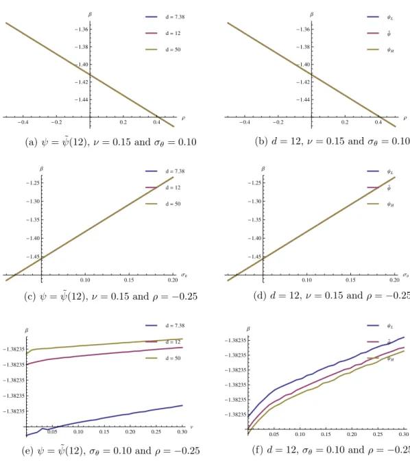
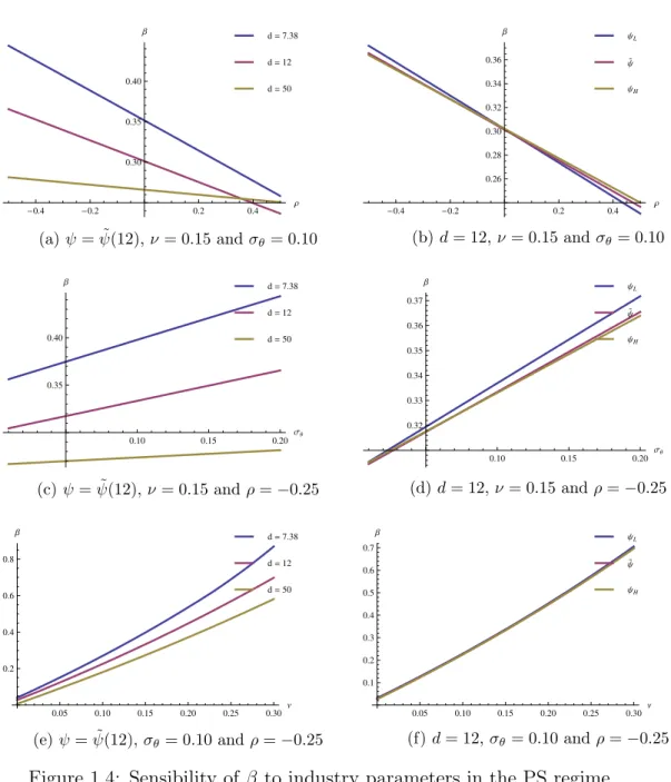
In the second-best regulation (SB), shown in Figure 1.2, the firm’s beta is slightly larger thenβF B across most of the parameter space, but it is fairly insensitive to industry characteristics. When the desutility of effort is held at its average value (panels 1.2a, 1.2c and 1.2e), wide variation in price-elasticity (different values of d) has a negligible impact on β, and changes in cost uncertainty (σθ) or market correlation (ρ) do not cause a change of more than 6 decimal points in β. Panels 1.2(b), 1.2(d) and 1.2(f) show that the impact of ψ is slightly more pronounced in the SB regime, but the influence of the remaining factor are still very small. In the second-best regime, in spite of having an informational disadvantage against the firm, the regulator is capable of allocating rents in a way that almost completely mitigates aggregate risk.
The situation does not change much when we remove the regulator’s abil-ity to observe ex-post costs. Under the WC regime, β is almost completely insensitive to demand elasticity and to the cost of inducing effort, as Figure 1.3 shows. As it might be expected, cost-related parameters have the larger (but still small in absolute magnitude) effect on β: raising cost uncertainty (standard deviation) from 1% to 20% raisesβ in 25 decimal points (regardless the choice of d or ψ); and as cost efficiency becomes more pro-cyclical (de-creasingρ from 0.5 to -0.5), β raises by a full decimal point. The end result however still resembles less restricted regimes such as the first and second-best, asβW C is never higher than -1 in any of the simulated scenarios. For the SB and WC systems, there does not exist a combination of parameters that significantly departures their equilibrium betas from βF B (of approximately -1.50 given our calibrated macro parameters).
re--0.4 -0.2 0.2 0.4 Ρ -1.47 -1.46 -1.45 Β
d=50 d=12 d=7.38
(a)ψ= ˜ψ(12),ν= 0.15andσθ= 0.10
-0.4 -0.2 0.2 0.4 Ρ
-1.48 -1.46 -1.44 -1.42 Β ΨH Ψ ΨL
(b)d= 12,ν= 0.15andσθ= 0.10
0.10 0.15 0.20
ΣΘ -1.50 -1.49 -1.48 -1.47 -1.46 -1.45 Β
d=50 d=12 d=7.38
(c)ψ= ˜ψ(12),ν = 0.15andρ=−0.25
0.10 0.15 0.20
ΣΘ -1.50 -1.48 -1.46 -1.44 -1.42 -1.40 Β ΨH Ψ ΨL
(d)d= 12,ν= 0.15andρ=−0.25
0.05 0.10 0.15 0.20 0.25 0.30Ν
-1.450 -1.448 -1.446 -1.444 -1.442 Β
d=50 d=12 d=7.38
(e) ψ= ˜ψ(12),σθ= 0.10andρ=−0.25
0.05 0.10 0.15 0.20 0.25 0.30Ν
-1.46 -1.45 -1.44 -1.43 -1.42 Β ΨH Ψ ΨL
(f)d= 12,σθ= 0.10andρ=−0.25
Figure 1.2: Sensibility ofβ to industry parameters in the SB regime.
-0.4 -0.2 0.2 0.4 Ρ -1.44 -1.42 -1.40 -1.38 -1.36 Β
d=50 d=12 d=7.38
(a)ψ= ˜ψ(12), ν= 0.15andσθ= 0.10
-0.4 -0.2 0.2 0.4 Ρ
-1.44 -1.42 -1.40 -1.38 -1.36 Β ΨH Ψ ΨL
(b)d= 12,ν= 0.15andσθ= 0.10
0.10 0.15 0.20
ΣΘ -1.45 -1.40 -1.35 -1.30 -1.25 Β
d=50 d=12 d=7.38
(c)ψ= ˜ψ(12),ν = 0.15andρ=−0.25
0.10 0.15 0.20
ΣΘ -1.45 -1.40 -1.35 -1.30 -1.25 Β ΨH Ψ ΨL
(d)d= 12,ν= 0.15andρ=−0.25
0.05 0.10 0.15 0.20 0.25 0.30Ν
-1.38235 -1.38235 -1.38235 -1.38235 -1.38235 Β
d=50 d=12 d=7.38
(e)ψ= ˜ψ(12), σθ= 0.10andρ=−0.25
0.05 0.10 0.15 0.20 0.25 0.30Ν
-1.38235 -1.38235 -1.38235 -1.38235 -1.38235 -1.38235 Β ΨH Ψ ΨL
(f)d= 12,σθ= 0.10andρ=−0.25
Figure 1.3: Sensibility ofβ to industry parameters in the WC regime.
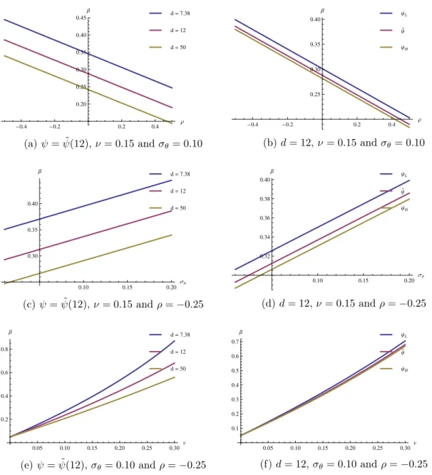
demand5, as we would expect. Third, the simulated betas are very close to the observed ones reported in Table A.1, specially when we consider average
5
For all practical purposes, we can safely ignore the regions with ρ > 0 in Figures 1.4(a) and 1.4(b) in whichβP S is larger for d= 50 thand= 12, i.e., when the expected
levels of demand and cost uncertainty in the simulation. Lastly, the numer-ical value of cost of inducing effort does not have a significant influence on βP S orβP C. This is a fortunate result, because although ψ plays a very im-portantqualitative role in the regulatory game, it is by far the most abstract parameter in the model and has no natural counterpart in the real world from where we can search for a representative numerical value. For the simulation exercise, we identified upper and lower bounds forψ that are consistent with meaningful equilibrium values for all regulatory regimes simultaneously, and found that β does not change significantly as we raise ψ fromψL toψH.
If we consider the different forms of second-best regulation (SB and WC) as one group, and the profit-sharing and price-cap systems as another, and compare their major numerical properties, two clear distinctions emerge. First, the responsiveness ofβ to changes in the market fundamentals is signif-icantly higher under the regimes where transfers are restricted. For example, the largest variation in β we were able to generate in the first group was 25 decimal points, as can be seen in Figures 1.3(c) and 1.3(d). On the other hand, there is a difference of approximately 80 decimal points among the low-est and highlow-estβ in some scenarios of the second group, as shown in Figures 1.4(e) and 1.5(e). Second, while in the first group cost-related variables (σθ and ρ) were the most influential onβ, in the second group demand variables (ν and d) play the major role. It seems that direct transfers are an effec-tive way to mitigate demand risk, and in the absence of such an instrument the systematic risk of the regulated entity is mainly influenced by demand uncertainty and price-elasticity.
1.4.2
Sensitivity of
β
to the Contract Space
-0.4 -0.2 0.2 0.4 Ρ 0.30
0.35 0.40
Β
d=50 d=12 d=7.38
(a)ψ= ˜ψ(12), ν= 0.15andσθ= 0.10
-0.4 -0.2 0.2 0.4 Ρ
0.26 0.28 0.30 0.32 0.34 0.36 Β ΨH Ψ ΨL
(b)d= 12,ν= 0.15andσθ= 0.10
0.10 0.15 0.20 ΣΘ
0.35 0.40
Β
d=50 d=12 d=7.38
(c)ψ= ˜ψ(12),ν = 0.15andρ=−0.25
0.10 0.15 0.20 ΣΘ 0.32 0.33 0.34 0.35 0.36 0.37 Β ΨH Ψ ΨL
(d)d= 12,ν= 0.15andρ=−0.25
0.05 0.10 0.15 0.20 0.25 0.30Ν 0.2
0.4 0.6 0.8
Β
d=50 d=12 d=7.38
(e)ψ= ˜ψ(12), σθ= 0.10andρ=−0.25
0.05 0.10 0.15 0.20 0.25 0.30Ν 0.1 0.2 0.3 0.4 0.5 0.6 0.7 Β ΨH Ψ ΨL
(f)d= 12,σθ= 0.10andρ=−0.25
Figure 1.4: Sensibility ofβ to industry parameters in the PS regime.
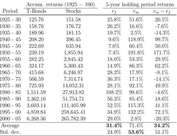
are only a price-tax rate pair (p, τ) that is constant across states. Finally, the most restricted contract is the price-cap (PC), in which no transfers are allowed and the contract specifies a single ceiling price p to be charged by the firm in every state.
-0.4 -0.2 0.2 0.4 Ρ 0.20 0.25 0.30 0.35 0.40 0.45 Β
d=50 d=12 d=7.38
(a)ψ= ˜ψ(12),ν= 0.15andσθ= 0.10
-0.4 -0.2 0.2 0.4 Ρ
0.25 0.30 0.35 0.40 Β ΨH Ψ ΨL
(b)d= 12,ν= 0.15andσθ= 0.10
0.10 0.15 0.20 ΣΘ
0.30 0.35 0.40 Β
d=50 d=12 d=7.38
(c)ψ= ˜ψ(12),ν = 0.15andρ=−0.25
0.10 0.15 0.20
ΣΘ 0.32 0.34 0.36 0.38 0.40 Β ΨH Ψ ΨL
(d)d= 12,ν= 0.15andρ=−0.25
0.05 0.10 0.15 0.20 0.25 0.30Ν 0.2
0.4 0.6 0.8 Β
d=50 d=12 d=7.38
(e) ψ= ˜ψ(12),σθ= 0.10andρ=−0.25
0.05 0.10 0.15 0.20 0.25 0.30Ν 0.1 0.2 0.3 0.4 0.5 0.6 0.7 Β ΨH Ψ ΨL
(f)d= 12,σθ= 0.10andρ=−0.25
Figure 1.5: Sensibility ofβ to industry parameters in the PC regime.
discrepancies to the varying level of flexibility in the space of contracts. In order to do that, we fixed all industry parameters at their average, represen-tative values, and calculated the equilibrium β under each policy and across the entire feasible range of each parameter at a time.
Figure 1.6 makes it clear why it is meaningful to classify the different regimes in two classes, one in which transfers are unrestricted (FB, SB and WC) and the other with PS and PC, as we did at the end of Section 1.4.1. Policies that belong to the second group are the only ones capable of generating positive betas, in line with the results obtained in Section 1.4.1. We can also the previous finding that, at least when measuring at average parameter values, β varies the most in the second group and by changing the level of demand uncertainty.
Another general conclusion that can be drawn is that the risk profile of each regime can be sorted in the same ordering that we have classified the regimes themselves, i.e.
βF B < βSB < βW C <0< βP S ≈βP C
so the simulation exercise suggests that contract flexibility, specially the abil-ity to operate transfers, significantly affect the regulated business’ β. How-ever, once we endogenize the optimal sharing ruleτ, we cannot tell whether the profit-sharing or the price-cap induce more risk to the business, as they appear to generate approximately the same profile of betas.
1.4.3
Sensitivity of
β
to Contract Power
In this section, we focus exclusively on the profit-sharing regime to assess the relationship between contract power and risk. Profit-sharing is the only system described in Section 1.3 in which the power of the contract can be explicitly obtained from the optimal policy. It is therefore the most natural choice to investigate the before mentioned relationship. In Figure 1.7, we plot the equilibrium values of risk (β) and power (1−τ) implied in the profit-sharing policy against each of the five industry parameters, while keeping the remaining four at their representative levels (d = 12, ψ = ˜ψ(12), σθ = 0.10, ν = 0.15and ρ=−0.25).
20 30 40 50 d -1.5 -1.0 -0.5 Β PS PC WC SB FB
(a) Sensibility tod
0.05 0.10 0.15 0.20 0.25 0.30Ν
-1.5 -1.0 -0.5 0.5 Β PS PC WC SB FB
(b) Sensibility to ν
0.10 0.15 0.20
ΣΘ -1.5 -1.0 -0.5 Β PS PC WC SB FB
(c) Sensibility toσθ
-0.4 -0.2 0.2 0.4 Ρ
-1.5 -1.0 -0.5 Β PS PC WC SB FB
(d) Sensibility to ρ
25 30 35 40 Ψ
-1.5 -1.0 -0.5 Β PS PC WC SB FB
(e) Sensibility toψ
20 30 40 50 d 0.3
0.4 0.5
Β,H1-ΤL
BetaHΒL PowerH1-ΤL
(a) Sensibility tod
0.10 0.15 0.20 0.25 0.30Ν
0.1 0.2 0.3 0.4 0.5 0.6 0.7
Β,H1-ΤL
BetaHΒL PowerH1-ΤL
(b) Sensibility toν
0.10 0.15 0.20
ΣΘ 0.35 0.40 0.45 0.50 0.55 0.60 0.65 Β,H1-ΤL BetaHΒL PowerH1-ΤL
(c) Sensibility toσθ
-0.4 -0.2 0.2 0.4 Ρ
0.4 0.5 0.6 Β,H1-ΤL BetaHΒL PowerH1-ΤL
(d) Sensibility to ρ
25 30 35 40 Ψ
0.40 0.45 0.50 0.55 0.60 0.65 0.70
Β,H1-ΤL
BetaHΒL
PowerH1-ΤL
(e) Sensibility toψ
Figure 1.7: Contract power and risk implied by PS regulation.
rises, power and risk also increase, monotonically.
One additional feature worth of comment is that, in our simulated econ-omy, the optimal power not only varies with demand conditions but it is also never greater than 80%, at least in the cases depicted in Figure 1.7. This implies that a pure price-cap mechanism, in which power is 100% whatever the market conditions or firm characteristics are, is rarely optimal.
1.5
Conclusions
We expanded, in a parsimonious way, the regulatory model of Laffont and Tirole (1986, 1993) to incorporate aggregate risk in the cash flows of the firm, and showed how the gradual introduction of restrictions in the space of contracts lead to an increase in the systematic risk of the firm. In incentive theory, from where the modern regulatory models were derived, the principal is usually allowed to operate direct transfers to the agent, but this ability prevents the model from generating sensible levels of risk to the firm. Only when the regulator is restrained from using this instrument we are able to reproduce CAPM betas like those observed for regulated companies in the real world.
By simulating our model, we managed to uncover the effect that major industry characteristics have on the risk of a regulated firm, and the results obtained were in line with the usual beliefs of how β is supposed to behave or respond to those characteristics.
Regulation and Return
Asymmetry
Regulated firms may be subject to some regulatory practices that potentially affect the symmetry of the distribution of their future profits. If these prac-tices are anticipated by investors in the stock market, the pattern of asym-metry in the empirical distribution of stock returns may differ among regu-lated and non-reguregu-lated companies. In this paper We review some recently proposed asymmetry measures that are robust to the empirical regularities of return data and use them to investigate whether there are meaningful differences in the distribution of asymmetry between these two groups of companies
Keywords: Economic regulation, skewness, non-parametric methods. JEL Classification: L51, G12
2.1
Introduction
Economic regulation is generally motivated on efficiency grounds, for instance as a response from a benevolent central planner to a market failure such as a natural monopoly. In those situations, a formally constituted regulatory institution, acting on behalf of the public interest, tries to emulate the condi-tions of a long-run competitive market equilibrium, in which industry partic-ipants earn a rate of return on their investment compatible with their cost of capital. There are certainly other reasons, not necessarily welfare enhancing or based on the public interest, that also gives rise to regulation. Stigler (1971) and Peltzman (1976) for instance suggested that regulatory institu-tions are the outcome of special interest groups that compete for political influence and the allocation of rents, in what has been called the capture theory of regulation.
In either case, the actions and policies of the regulator have a direct and profound impact on the profitability and risk of regulated entities. Peltzman argued that the regulatory process attenuates profit fluctuations, so the risk of the firm decreases when regulation becomes more stringent. This “buffer-ing” hypothesis has been interpreted as a reduction in the variance of profits and possibly on the (CAPM) beta of the regulated firm. This hypothesis was tested by several authors, e.g. Norton (1985) and Davidson, Rangan and Rosenstein (1997), and it seems to be valid at least in sectors under low-powered regulation. High-powered (incentive-based) regulatory systems such as the price-cap seem to impose more risk on the firm, as claimed for instance by Alexander, Mayer and Weeds (1996) and Grout and Zalewska (2006) who find a positive relation between contract power (incentives for cost reduction) and beta.