UNIVERSIDADE TÉCNICA DE LISBOA INSTITUTO SUPERIOR DE ECONOMIA E GESTÃO

(1)

UNIVERSIDADE TÉCNICA DE LISBOA

INSTITUTO SUPERIOR DE ECONOMIA E GESTÃO

MESTRADO EM:

Finanças

Volatility Forecasts and Value-at-Risk estimation using TGARCH

model

Sandra Cristina Rosa Ruivo

Orientação:

Prof. Doutor João Carlos Henriques da Costa Nicolau

Júri:

Presidente:

Prof. Doutor João Luís Correia Duque

Vogais:

Prof. Doutor João Carlos Henriques da Costa Nicolau

Prof. Doutor José Joaquim Dias Curto

(2)

(3)

Volatility Forecasts and Value-at-Risk estimation using TGARCH

model

Sandra Cristina Rosa Ruivo

Abstract

Value-at-Risk (VaR) has emerged in recent years as a standard tool to measure and control the risk, mainly the market risk, of financial portfolios. It measures the worst loss to be expected of a portfolio over a given time horizon at a given level of confidence. The calculation of Value-at-Risk commonly, involves estimation of the volatility return price and quantile of standardized returns.

In this paper, two parametric techniques were used to estimate the volatility of the returns (market prices) of a Portuguese Financial Institution portfolio. Although to achieve the quantiles of standardized returns, both parametric technique and one nonparametric technique were considered. The quality of the measuring result was analysed through the backtesting technique for the forecasting multiperiod.

In this study it is revealed that AR(1)-TGARCH methodology produces the most accurate VaR forecast, for one day holding period. The volatility forecasts for the two other holding periods, considering the three methodologies, revealed to be biased.

Key words: Market Risk, Value-at-Risk, Volatility, Forecasting, TGARCH, Backtesting

(4)

Index

Abstract……….….. 3

Index……….…… 4

List of Tables……….……. 5

List of Pictures……….….. 6

1. Introduction……….… 7

2. Literature Review………..….….. 10

3. Technical Background and Data analysis………. 18

3.1 Estimating Volatility………..……. 18

3.1.1 Historical Simulation…………..……….……. 20

3.1.2 RiskMetrics….………….………..……….….. 20

3.1.3 AR(1)+TGARCH………..……… 20

3.2 Estimating Value-at-Risk………. 24

3.2.1 Historical Simulation…………..……….……. 24

3.2.2 RiskMetrics…...………..………... 25

3.2.3 AR(1)+TGARCH………..……… 26

3.3 Backtesting………..……….……….. 29

3.4 Data analysis……..……….……….. 31

4. Estimation Results………..……. 34

5. Main Findings………. 38

References……….………..……….. 41

Appendix

(5)

List of Tables

Table 1 – Statistics TGARCH Model Eviews Output ……...……… 23

Table 2 – Return Statistics for the entire sample………. 33

Table 3 – Parameters estimated for Normal distribution and for t-Student distribution….. 33

Table 4 – TGARCH Model Eviews Output……….………...…. 34

Table 5 – Backtesting Results for one holding period……….. 35

Table 6 – Backtesting Results for one week holding period……… 36

Table 7 – Backtesting Results for two weeks holding period……….. 37

Table 8 – Value-at-Risk for one day holding period, 5% confidence level………. 39

Table 9 – Value-at-Risk for one day holding period, 1% confidence level………. 39

(6)

List of Figures

(7)

1. Introduction

During the 90’s, the financial world watched the fail of many large institutions, see

Jorion (1997), due to the exposures to specific movements in the financial market. The

instability in emerging markets, starting in Mexico in 1995, continuing in Asia in 1997, and

spreading to Russia and Latin America in 1998, plotted the interest in Risk Management

best practice.

These financial disasters brought clearly, to the financial world, the need to control

financial risks. The regulatory authorities imposed the Risk-Based-Capital adequacy

requirements on financial institutions (see Dimson and Marsh, 1995; Wagster, 1996).

Consequently, good measures of risk have come into focus, and Risk Management

became of supreme importance in the finance industry, especially for Institutional Investors

such as Pension Funds, Insurance Companies and as well Asset Management Firms that

manage funds on their one.

The need to determine the amount of risk, achieve the sense of the possibility of

losses and measuring the risk accurately, turned out to be a critical matter for Financial

Institutions.

The possible extent of a loss caused by an adverse market movement over the

next day or next few days/months given the current volatility background, generally

associated with the market risk of a given portfolio, became, especially for Risk Managers,

(8)

For Risk Managers the main question turns out to be: how can we quantify risk;

how much capital do we need to cover the risks under our business?

Theoretically, there are several possibilities: standard deviation, quantiles,

interquantiles range or shortfall measures. Value-at-Risk (VaR), a quantile measure, has

been the preferred tool in financial industry. Following the 1995 Basle Committee

agreement, the Value-at-Risk (VaR) has turned into the standard risk measure adopted to

define the market risk exposure of a financial position.

Nowadays, for Insurance Companies, Value-at-Risk (VaR) is a standard tool which

quantify, with a certain confidence level, for a certain time period, the maximum anticipated

loss in portfolio value due to adverse market movements. As providers of financial security

the need to control the financial risk grows in order to provide protection and economic

security to policyholders.

The actual European Capital Solvency Requirement, regulating the insurance

activity, is not sufficiently sensitive to risk. A new risk based regulatory framework is under

developing - Solvency II (see Swiss Re, Sigma n. º4, 2006). This new system gives special

attention to the development of internal models which identify and capture the principal risk

factors under the insurance activity (market, underwriting, operational and credit risk).

Market Risk is, generally, the highest risk for a life Insurance Company.

Using a real Portuguese Life Insurance portfolio, this dissertation aims to measure

(9)

using three different methodologies, two parametric techniques (RiskMetrics and

TGARCH) and one non parametric technique (Historical Simulation).

Value-at-Risk was estimated for two different confidence levels,

α

=5% and %

1

=

α

for three forecasting holding time periods; one day, one week and two weeks.

The three methodologies revealed to be a good VaR estimator for one day

forecasting period, excepting Risk Metrics with 1% of confidence level. There is evidence

that for all methodologies the final results are biased for the forecasting holding periods,

five and ten days.

This study is structured as follows: Section 2 categorizes parts of the existing

literature under the methodology. The theoretical background and data analysis are

described on section 3. On section 4 the estimation results are presented. Section 5

(10)

2. Literature Review

The development of models for measuring forecasting volatility began with Engle

(1982). Many findings resulting of Engle’s original work had huge implications on actual

risk management techniques.

One of those was the important contribution of the RiskMetrics by J.P.Morgan

(1996) methodology: the introduction of the Value-at-Risk (VaR) concept. The new

concept, as mention by Christoffersen, Hahn and Inoue (2001) «transforms the entire

distribution of the portfolio returns into a single number, which investors have found useful

and easily interpreted as a measure of market risk».

The object of VaR is to determine a distribution of the end-of-period portfolio taking

into account the probable changes in the market risk factors, research in this matter is

reported in Dowd (1998) and Duffie and Pan (1997).

Ahlgrim (1999) defined Value-at-Risk (VaR) as a probabilistic measure of the

losses that are expected over a period of time under normal market conditions. Given a

confidence level defined by a probability, losses over the defined horizon will exceed the

VaR only a small percentage of the time. VaR is essentially a

α

-percentage quantile of

the conditional distribution of the portfolio returns.

In actuarial terms, Wirch (1999) defines VaR, or VaR capital requirement, as

quantile reserve, often using the 5% percentile of the loss distribution, using the empirical

(11)

In spite of its definition, the main goal of VaR is to quantify the uncertain amount

which may be lost on a portfolio over a given period of time with a certain confidence level.

There are several models for calculating VaR. The existing models differ in the

methodology they use, the assumptions they make and the way they are implemented.

VaR models can be particularly different in the way they address the problem of the

portfolio estimation, leading to the essential question: how to forecast the quantiles?

The different approaches that are used to model their variability distinguish VaR

methodologies (see Manganelli and Engle, 2001);

i) Non Parametric (Historical Simulation);

ii) Parametric (Risk Metrics and GARCH);

iii) Semiparametric (Extreme Value Theory – EVT)

During several years, Risk Managers preferred choice was the use of non

parametric techniques, mainly the Historical Simulation (HS) for estimating VaR (see

Giannopoulos, 2002). Based on the return of the portfolio value, VaR is the percentile that

corresponds to the VaR probability. The changes in the risk portfolio are associated only

with the historical experience of the portfolio. For this non-parametric methodology, the

final quantiles are under the assumption that any return in a particular period is equally

likely. This method is relatively simple to implement since it does not make any

distributional assumption about portfolio returns (see Danielsson and Vries, 1997; Dowd,

1998; Manganelli and Engle, 2001). It does not specify any assumptions about valuation

(12)

The main problem with this technique is that VaR predictions consider all historical

data equally relevant. As mention by Manganelli and Engle, (2001), «the distribution of

portfolios returns does not, therefore, change within the window». Giannopoulos (2002)

referred «that leaving out the highly volatile market conditions that may have occurred a

little earlier than the beginning of the data window will make a huge difference in VaR

prediction».

Historical simulation is based on an independent and identically distributed (i.i.d.)

assumption, which is known to be incorrect under financial data; this limitation is seen in

Sarma (2003).

Regarding the parametric models, Financial Institutions are using ARCH

(autoregressive conditional heteroscedasticity) models and the related GARCH

(generalised autoregressive conditional heteroscedasticity) formulations because they

capture volatility persistence in a simply way (see Duffie and Pan, 1997). Models such as

RiskMetrics and GARCH offer a specific parameterisation for the behaviour of returns (see

Manganelli and Engle, 2001).

The ARCH models were introduced by Engle (1982) and express the conditional

variance as a linear function of the past squared innovations (see Angelidis, Benos and

Degiannakis , 2003).

A high order for the ARCH process was needed in order to grab the dynamic of the

(13)

ARCH (GARCH) developed by Bollerslev (1986) was the answer to the infinite

parameters.

In GARCH models the conditional variance depends not only on the latest

innovations, but also on the previous conditional variance. The simplest GARCH model is

given by

2 1 2

1 2

) 1 , 0 .( . . ~

−

− +

+ = =

t t

t

t t t t

u

d i i u

βσ

α

ω

σ

ε

σ

where

σ

_t₋₁2 is the conditional variance using information up to time t-1 and u_t₋₁ the latest innovations. To achieve the conditional variance positive the following conditions must be

verified,

ω

>0 and

α

,

β

≥0.

In these models the sum of parameters

α

+

β

measures the persistence. The

persistence parameter indicates the rate at which the multiperiod volatility forecast reverts

to its unconditional mean (see Campbell, Lo and Craig, 1997).

The particular specification of the variance equation and the assumption

ε

_t i.i.d.,

are the two essential elements of the model. The first one it is due to the characteristics of

financial returns and the second one is a necessary mechanism to estimate the unknown

parameters (see Manganelli and Engle, 2001). An additional step is the specification of the

distribution of the u_t. The most used distribution is the standard normal (see Nicolau, 2007). After this distribution assumption being defined, becomes possible to write down a

likelihood function and get an estimate of the unknown parameters (see Manganelli and

(14)

The flexibility of ARCH modelling produced the developing of several volatility

models. Extensive researches have focused on evaluating other volatility measures that

improved conditional volatility forecasts. Developed by Glosten, Jagannathan and Runkle

(1993), the GJR-GARCH as well known Threshold GARCH (T-GARCH), is the most

common model used among asymmetric volatility. It was proposed using a dummy

variable for negative shocks in the GARCH model.

Shock returns volatility reacts differently to positive and negative movements but

generally when the asset price rises up, the variance of the return gets down. Although,

daily returns are uncorrelated while the squared returns are strongly autocorrelated, letting

that periods of persistent high volatility are followed by periods of persistent low volatility.

This is the so called asymmetric effects, one of the most important characteristic of the

financial data. Black (1976) called this phenomenon as Leverage Effect.

The RiskMetrics technique is a particular case of the GARCH family; the volatility

under this parametric technique uses a particular autoregressive moving average process:

Exponentially Weighted Moving Average (EWMA), for the price model, representing the

finite memory of the sample.

RiskMetrics follows the assumption that returns are conditionally1_normally

distributed. This approach is a special case of the GARCH (1,1) process, where

ω

=0 and

α

+

β

=1,

σ

t2 =

λσ

t2₋₁+(1−

λ

)ut2₋₁.

1_{Conditionally means: conditional on the prices set at time t, which usually consists of the past returns prices}

(15)

RiskMetrics considers the parameter of the model: λ (0< λ<1), usually set equal to

0.94 for daily data or 0.97 for monthly data, and assumes that standardised residuals are

normally distributed, see J.P.Morgan (1996).

Under RiskMetrics methodology, VaR measure has only a few unknown

parameters, which are simply calibrated and work quite well in common situations.

However, several studies such as Christoffersen (1998) and Danielsson and Vries (1997)

have found significant improvements when some modifications from the rigid RiskMetrics

were explored.

Among the literature, the main findings related to both GARCH and RiskMetrics

refer that both underestimate the VaR. This is due to the assumption of normality of the

standardised residuals that are not quite consistent with the general behaviour of financial

returns. There are some study’s were these methods allow a complete identification of the

distribution of returns and were an improvement of their performance has been achieved

putting normal distribution assumption aside, see McNeil, and Frey (2000).

An alternative measure of market risk has been proposed, namely Extreme Value

Theory (EVT). According to Sousa (1999), EVT is the appropriate methodology for tails

with significant levels equal or less than 1%. According to his study, the semi parametric

technique EVT is the best practice to model stress situations and also atypical situations.

As shown, for instance, in Danielsson and Vries (1997), models based on

conditional normality are not well-matched to estimating large quantiles. The estimation of

(16)

issue that has originated several works; see Embrechts (1998), Lauridsen (2000),

Manganelli and Engle (2001).

The purpose of this dissertation was not to test the use of small confidence levels,

therefore the EVT via was not used; however literature references are mentioned for this

matter.

The most common time horizons used by commercial and investment banks to

achieve VaR’s are one day, one week, and two weeks. The Basle Committee and Banking

Supervision (2001), mandate that banks using VaR models should control market risk

using a holding period of two weeks and a confidence level of 1%. On the opposite,

Institutional Investors holding long periods VaR figures are performed from one month to

several years. The time horizon or the holding period can vary a lot in different

applications; see Christoffersen (2001) and Jorion (1997).

If VaR is used to establish capital requirements, then regulators must decide the

appropriate time of period ahead. As asset management firms, given the conservative

view of accounting and its focus on liquidation values, it is appropriate to have a capital

standard based on a short time period, such as one month or less. For example, due to

the long-term of life insurance contracts it raises a potential difficulty in determining the

appropriate time for a VaR calculation. The use of daily data to estimate volatilities among

assets may not be valid over long time horizons. Giannopoulos (2002) refers the main

(17)

Backtests first performed by J.P.Morgan (1996) determine that Risk Managers

should back test all models. Illustrated by the Basel rules, the Backtesting technique will

evaluate how a model actually performed for a given period versus what was predicted,

representing how often the actual losses have exceeded the level predicted by VaR.

Backtesting will verify the accuracy, certifying that models are not systematically biased.

Even being one of the best practices in financial market, Value-at-Risk has some

established criticisms. VaR only gives the upper value of the losses that can occur with a

given frequency and, VaR does not reflect the potential size of the loss given that a loss

exceeding the upper bound has occurred. Artzner (1999) shows that VaR as a measure of

market risk has various theoretical deficiencies; Artzner refers «this situation in general

occurs in portfolios containing non linear derivatives». Other critical statements related to

(18)

3. Technical Background and Data analysis

The aim of this dissertation is to evaluate the three methodologies (one non

parametric and two parametric techniques) to measure Value-at-Risk, evaluating if they

are good VaR estimators. The next chapters tend to resume the technical background and

the data analysis used to achieve the final goal.

3.1. Estimating Volatility

Let P_t be the price of a portfolio at a time t. The observed return at time t is given by rt =ln(Pt /Pt₋₁), denoting the continuously compound rate of the return from time t-1 to

t. For a holding period h, the aggregate return at time t can be written by

Rt_,h =ln(Pt₊h₋₁/Pt₋₁)=rt +...+rt₊h₋₁.

The historical information produced by the process

{ }

P_t , namely the ℑ_t, is the σ -algebra generated by P_t,P_t₋₁,....The value of the portfolio at time t+h will be

) exp( _t ₁_,_h t

h

t P R

P₊ = ₊ .

According to Value-at-Risk definition, the potential loss of a portfolio over a

predetermined holding period h with a predefined confidence level (1-

α

), see Dowd

(1998), is mathematical defined by,

prob(R_t₊₁_,_h >q_t₊₁_,_h|ℑ_t)=1−

α

(19)

prob(R_t₊₁_,_h <q_t₊₁_,_h |ℑ_t)=

α

, were, q_t₊₁_,_h is the

α

-quantile of the conditional distribution of Rt+1,h.

VaR, with a probability of

α

, is given by VaR =P_tq~_t₊₁_,_h (see Dowd, 1998 and Jorion, 1997). At time t, P_t is known, the unknown figure is the quantile of the conditional

distribution. Several methods could be considered; in this study three different

methodologies were used.

In practice, the selection of h≠1 period makes some complications in the

estimation of VaR, see Wong and So (2001). Being F_n_,_t(.) the cumulative distribution function for h-period return Rn,h given ℑt, i.e., Fn,t (x) = Pr(Rn,h ≤x|ℑt).

To achieve VaR, the inverse of Fn,t (.) for a certain confidence level is needed. As

referred by Nicolau (2007) and Wong and So (2001), Fn,t (.) is generally intractable,

especially when h is large. The conditional distribution of Rn,h given ℑt is written as

) ,...., (

) | ( ) |

( )

( 1 ₁

1 1

1 ,

, , n n h

h

i

i n i n h

n h n R

h

n x f R f r d r r

F _n_h _x ₊ ₊

−

= + +−

− +

∫

ℑ

∏

ℑ

= _≤ .

The evaluation of the inverse of the error distribution has to involve high-dimension

integration. Generally the exact value is usually unavailable when h is greater then one.

As referred by Nicolau (2007) and Wong and So (2001) that will be adopt in this

(20)

[

] [

]

(

nh n nh n

)

n h

n NER R

R_, |ℑ ~ _, |ℑ ,var _, |ℑ

3.1.1. Historical Simulation

According to this non-parametric method, the changes in the risk portfolio are

related with the historical past experience of the portfolio. The final quantiles imply the

assumption that any return in a particular period is equally likely. This method is relatively

simple since it doesn’t make any distributional assumption about portfolio returns. The past

returns are used to predict future returns, see Danielsson and Vries (1997). Some details

under the historical volatilities can be seen also in Duffie and Pan (1997).

3.1.2. RiskMetrics

The estimation of volatility using the RiskMetrics technique for one period return is

defined by 2

1 2

1

2 ₍₁ ₎

−

− + −

= t t

t

λσ

λ

r

σ

with

λ

=0.94. By iterating it comes,

{

....

}

) 1

( 2

3 2 2

2 2

1

2 ₌ ₋ ₊ ₊ ₊

− −

− t t

t

λ

r

λ

r

λ

r

σ

reflecting the exponential smoothing. For multiple

periods return, the square root is frequently used

σ

_t₊_h_|_t = h

σ

_t₊₁_|_t.

3.1.3. AR(1)+TGARCH

(21)

[

t t

]

t

t Er u

r = |ℑ₋₁ + , where ℑt₋₁ is the available information at time t-1,

µ

t =E

[

rt |ℑt−1

]

is the conditional mean and u_t is the unpredictable part, or also known as the innovation process.

The predictable component, conditional mean return was considered as a k-th

order autoregressive process, AR(k), defined by

[

t t

]

t t k t k

t E r c r r r

k

AR( )⇒

µ

= |ℑ₋₁ = +

φ

₁ ₋₁+

φ

₂ ₋₂+...+

φ

₋ .

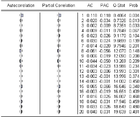
The autocorrelation (AC) and partial autocorrelation (PAC) functions were

analysed, using the Eviews2_{, to achieve the specify order lag, characterizing the pattern of}

the temporal dependence in series. By definition the PAC of a autoregressive process of

order k, AR(k), cuts off at lag k.

From Figure1 below, the output from the Eviews, provides some evidence that time

series considered is a 1-th order autoregressive process, AR(1) or a 1-th order moving

average process, MA(1). For lags higher then one, the autocorrelation is within the

bounds, which means it is not significantly different from zero at a 5% confidence level.

Due to the final results AR(1) provides the best out-of-sample forecast for the studied

portfolio. Therefore the predictable component, was considered as a 1-th order

autoregressive process, AR(1).

(22)

Figure 1 – Auto and Partial correlations - Eviews output

The unpredictable component was expressed as an ARCH model,

σ

2t is the

conditional variance, being positive, changing with time and is a measurable function at

time t-1, see Angelidis and Benos and Degiannakis (2003).

Thus, the final model used was specified as:

t t

t c r u

r = +

φ

₋₁+

) , 0 ( ~

| 2

1 t

t

t N

u ℑ₋

σ

t t t

(23)

In order to capture the asymmetry exhibited of returns, reflecting the effect of good

and bad news on volatility, the so called GJR-GARCH model, developed by Glosten, and

Jagannathan and Runkle (1993), was developed, and is defined by,

{ } 21 2 1 2 1 2 0 1 − −

− + Ι +

+

= t t u₋_< t

t

ω

α

u

γ

u t

βσ

σ

, where

{ }    ≥ < = Ι − − <

− 0 0

0 1 1 1 0 1 t t u u if u if

t .

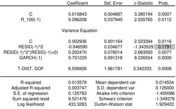
For the time series considered in this study, the positive model variations, which

are good news, are not statistically significant for a 5% confidence level, see below table 1,

output of Eviews. The positive variations do not influence the volatility under this portfolio.

Table 1 - Statistics TGARCH Model EVIEWS Output

Dependent Variable: R_100

Method: ML - ARCH (Marquardt) - Student's t distribution Sample (adjusted): 2 610

Coefficient Std. Error z-Statistic Prob.

C 0.015843 0.004687 3.380194 0.0007

R_100(-1) 0.096208 0.037940 2.535765 0.0112

Variance Equation

C 0.002936 0.001164 2.523394 0.0116

RESID(-1)^2 -0.046590 0.034677 -1.343529 0.1791 RESID(-1)^2*(RESID(-1)<0) 0.202470 0.076014 2.663593 0.0077

GARCH(-1) 0.751229 0.091318 8.226554 0.0000

T-DIST. DOF 6.556926 1.961781 3.342333 0.0008

(24)

Therefore, the final model used in this study was a particular GJR-GARCH model,

{ } 21 2

1 2

0

1 −

−Ι +

+

= t u₋_< t

t

ω

γ

u t

βσ

σ

,

where { }    ≥ < = Ι − − <

− 0 0

0 1 1 1 0 1 t t u u if u if t .

3.2. Estimating Value-at-Risk

3.2.1. Historical Simulation

The Historical Simulation (HS) approach simplifies the procedure to obtain

Value-at-Risk. No distribution assumption is needed and, as previously mentioned, the past

returns are used to predict future returns. VaR at a

α

% confidence level will be the

α

% quantile of the worst outcomes. If the corresponded number falls between two consecutive

returns, then an interpolation rule is applied (see Manganelli and Engle, 2001).

Mathematically, VaR for one holding period is defined by, see Nicolau (2007),

α

α ℑ =

− <

− +

+ | )

(P_n ₁ P_n VaR_n_,_n ₁_, _n

prob ⇔ prob(R_n₊₁P_n <−VaR_n_,_n₊₁_,_α |ℑ_n)=

α

⇔

⇔ _<− + α _ℑ ₌

α

+ | )

( , 1,

1 n n n n n P VaR R

prob ⇔ prob(R_n₊₁<q_α |ℑ_n)=

α

,

(25)

) (

) |

(r ₁ q_α prob r ₁ q_α

prob _n₊ < ℑ_n = _n₊ < ,

Value-at-Risk can be estimated, VaˆR_n,_n+1,_α =−q~_αP_n where the Pn represents the portfolio amount at time t, and q~_α represents the empirical

α

-quantile of the returns

{

Rn+h(h),n=1,2,...

}

.

3.2.2. RiskMetrics

To achieve VaR through the RiskMetrics methodology, according to J.P.Morgan

(1996), two different steps must be carried out. The first one requires the need to estimate

the volatility for holding portfolio for one day before converting it into the volatility for

multiple days. The second one requires the compute of the quantile of the standardised

return processes, based on the assumption that the process follows a standard normal

distribution.

For one holding period, the daily VaR, for the confidence level

α

, 5% and 1%, is

calculated by multiplying the volatility estimated on a given day, with the (1-α) quantile of

the standard normal distribution, according to RiskMetrics techniques.

To achieve a multiperiod forecast it applies the use of the “squared-root-of-time”;

t t t

h

t+ | = h

σ

+1|

σ

derived on the assumption of uncorrelated returns, see J.P.Morgan

(1996).

(26)

3.2.3. AR(1) + TGARCH

The GJR-GARCH model considered in this study is given by,

t t

t c r u

r = +

φ

₋₁+ , with

t t t

u =

σ

ε

σ

_t2 →TGARCH

{ } 21 2

1 2

0

1 −

−Ι +

+

= t u₋_< t

t

ω

γ

u t

βσ

σ

, (volatility)

where { }    ≥ < = Ι − − <

− ₀ ₀

0 1 1 1 0 1 t t u u if u if t .

Under the ARCH models the maximum likelihood estimation is frequently used.

Following the assumption, for (r_t −

µ

_t), of independently and identically distributed standardized innovations (i.i.d.), and being f the density function, the log-likelihood function

based on standardised t-student distributed innovations is given by

∑

= = n t t L L 1 ) ( )

(

θ

, where

2 1 2 2 1 2 1 2 2 1 ) 2 ( 1 log ) | ( log ) ( + − −               −       ₋ +       Γ       + Γ         − = ℑ = ν

ν

σ

ν

π

σ

θ

t t t t t t t r y r f L

(

2

)

log 2 1 log 2 1 log 2

1 2 ₋ ₋ ₋

−

=

σ

t

π

ν

        ₋ − + + −       Γ       ₊ Γ

+ ( ₂ )2

(27)

(.)

Γ is the Gamma function and

ν

is the number of degree of freedom, and

µ

_t,

σ

_t2

are the conditional mean, and variance of the model respectively. Under this model the

unknown parameters are denoted by

θ

. To achieve the real parameter vector, the

maximum likelihood estimator

θ

ˆ, is obtained by maximizing the equation above.

The unknown parameters for the presented model are

θ

=(c,

φ

₁,

ω

,

γ

,

β

,

ν

)′ under the usual restrictions of the GARCH models, and with

γ

>0.

The distribution of the quantile for h=1 (one period forecasting) is known (z_α), under the studied model, is a t-Student (standardised), but for periods higher than one the

distribution is generally unknown. Regarding literature, for h>1, the quantile of the normal

distribution was taking into account.

Following the assumption that the conditional portfolio returns for h>1 holding

periods has a normal distribution (see Nicolau, 2007);

[

]

[

]

(

n h n n h n

)

n h

n h NEr h r h

r ₊ ( )|ℑ ≈ ₊ ( )|ℑ , var ₊ ( )|ℑ

leads to

[

n h n

]

[

n h n

]

n h

n

n Er h z r h P

VaR , + ,α =−( + ( )|ℑ + α var + ( )|ℑ ) .

It is known that

[

rn h h n

]

n n n hn

E ₊ ( )|ℑ =

µ

₊₁_, +...+

µ

₊ _, , working with a AR(1) structure

n h h

n h

n c

_φ

φ

y

φ

µ

+

− − =

+ ₁

1

(28)

therefore,

[

]

n

h h

n n

h

n h c y c y

r E

φ

₊ − − + + + − − = ℑ + 1 1 ... 1 1 | )

( 1 1

using the Mathematica Software, the following is obtain;

[

]

₂

) 1 ( )) 1 ( ) 1 ( ( ) 1 ( ) 1 ( | ) (

φ

+ − + − + − + + − + − = ℑ + h h n n h n h c y h r E .

It was also necessary to calculate thevar

[

rn+h(h)|ℑn

]

. For the specific model in this study

{ } 21 2

1 2

0

1 −

−Ι +

+

= n u₋_< n

n

ω

γ

u n

βσ

σ

for one period forecasting, it comes

{ } 2

2 2

,

1n n u 0 n

n

ω

γ

u n

βσ

σ

+ = + Ι _< +

for two periods forecasting,

2 , 1 2

,

2n ₂ n n

n+  +

     + +

=

ω

γ

β

σ

for h forecasting periods,

2 , 1 2

,n n h n

h

n+ =

ω

+

δσ

+ −

σ

, where

δ

=

γ

+

β

2 iterating 2

,n h n+

σ

in order of 2 , 1n n+

σ

, it appears

) 1 ( 1 2 , 1 1 2

,

ω

_δ

δ

σ

ω

_δ

σ

+ − + + = − +

+ n n

h n

(29)

[

]

∑ ∑

= + − − = + _                   + − + −         = ℑ h k n n h k h j j n h n h r 1 2 , 1 1 2

0 1 1

| ) ( var

δ

ω

σ

δ

ω

φ

through the use of the Mathematica Software, var

[

r_n₊_h(h)|ℑ_n

]

reduces to

(

+ + − − + − + + − + − − + − + + − + − − + +

δ

ω

δ

σ

φ

ω

δ

φ

1 ) 1 ( ) 1 ( 1 ) 2 )( 1 ( ) 1 ( ) 1 ( 1 2 , 1 2 1 2 h h n n h h h

)

                −         −       − −         −       − + + + +

+

_φ

_δ

φ

δ

φ

δ

φ

δ

φ

δ

σ

ω

1 2 1 )) 1 ( ( 1 2 2 2 2 2 , 1 h h h h n n x

(see Nicolau, 2007, section 11.3.3).

3.3. Backtesting

The main goal was to test and analyse the three different approaches for the

forecasting techniques, in a risk management atmosphere, i.e, measuring risk. The quality

of the volatility forecasts and the respectably independence on forecasts will affect the

quality of the forecasted VaR. The purposes of Backtests methodology is to monitor VaR

forecasts and after that evaluate volatility models, being sure that models are not

systematically biased.

Backtesting tests will verify volatility forecasts as good VaR estimators testing the

rule that the values exceeding VaR are independent and identically distributed (being a

(30)

Introduced by Christoffersen, Diebold and Schermann (1998), the likelihood ratio

test was created for testing the independence, and also for testing the

[ ]

α

⇔ =

=

= t

t EI

I

prob( 1) , generally known by correct unconditional coverage, where

t

I is the indicator event. The indicator event is defined as the returns that exceed VaR by

   − ≥ − < = − − α α , 1 , , 1 , 0 1 t t t t t t t VaR r if VaR r if I .

For testing the independence, one of the possible ways can be through the known

runs test, the hypothesis testing is H0 :

{ }

It is independent and identically distributed (i.i.d), see Nicolau (2007). For samplings with n₀ >20 or n₁>20 the statistic test is given by

(

Z zobs

)

prob > , where

[ ]

(0,1)

var X N

X E X

Z ₌ − __→d _{, with}

[ ]

₌2 0 1₊1

n n n X

E and

[ ]

) 1 ( ) 2 ( 2

var 0 1₂ 0 1

− − = n n n n n n n X .

The limits under X are;

{

}

{

}

   ≠ + = = 1 0 1 0 1 0 1 0 1 , min 2 , min 2 max n n if n n n n if n n X .

The sampling figures are represented by n=n₀ +n₁, with n₀,n₁ number of zeros and ones, respectively.

(31)

0 1

) ˆ 1 ( ˆ

) 1 ( log

2 _n _n

n n

LR

α

− − −

= , with

n n₁

ˆ =

α

, α is the defined

confidence level, 5% or 1%.

Under the null hypothesis, the statistic test LR is approximately distributed to 2 1

χ

,

chi-squared distribution with one degree of freedom (see Nicolau, 2007). For analysing the

statistics tests it is equivalent to analyse the p-value.

3.4. Data analysis

A real Portuguese Life Insurance portfolio was used. This portfolio is linked to

several financial assets; stocks, stock indices, foreign currency, etc. For simplicity, in this

dissertation it was assumed as a unique portfolio risk.

The daily figures were obtained from 22nd_{of June 2004 until 28}th_{of November}

2006, before this data there were no daily figures available on the system of the company,

only monthly figures. Excluding weekends and holidays in Portuguese market were used

610 returns. Following Nicolau, (2007), it was considered continuous returns. The final

returns were considered times 100 (R_100), due to the use of the software Gauss routine.

Most of the contracts will end during this current year, and the totally at the end of the next

year. For the asset management firm that manages funds, the control of the market risk is

empirical. Therefore this dissertation aims to study if the volatility measures can be used to

(32)

Three different methodologies were used to achieve Value-at-Risk for two different

confidence levels, 5% and 1%, and forecasted for three holding periods, one day, one and

two weeks. The final conclusion about volatility measure was achieved through the

Backtesting technique.

As defined on the technical background, the P_n represents the portfolio amount at time t. For simplification in this study the portfolio amount was considered equal to one.

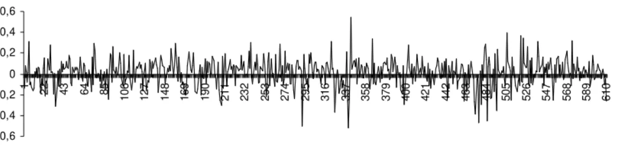
The total 610 returns are presented on figure 2 below,

Figure 2 - Portfolio daily Returns

-0,6 -0,4 -0,2 0 0,2 0,4 0,6

1 ₂₂ ₄₃ ₆₄ ₈₅

10 6 12 7 14 8 16 9 19 0 21 1 23 2 25 3 27 4 29 5 31 6 33 7 35 8 37 9 40 0 42 1 44 2 46 3 48 4 50 5 52 6 54 7 56 8 58 9 61 0

The volatility clusters (Leverage effect), strong (weak) variations are more probable

to be followed by strong (weak) variations, are generally associated to financial data, the

evidence on the portfolio returns studied is noted.

The table 2 below shows a negative skewness, meaning the distribution is

asymmetric, having heavier tails. The kurtosis exceeds 3, generally the kurtosis of the

normal distribution, meaning that distribution is leptokurtic relative to the normal (see

(33)

Table 2 - Return Statistics for the entire sample

Observations Mean Variance Maximum Minimum Kurtosis Skewness Jarque-Bera Prob.

R_100 610 0,01429 0,01589 0,54428 -0,52027 4,9222 -0,3477 1,0621 0,000

Table 2 summarises the main statistics and also the Jarque-Bera Statistic used for

testing normality. The null hypothesis of normality is rejected at any level of confidence,

combined with the evidence of the kurtosis higher than three and the negative skewness.

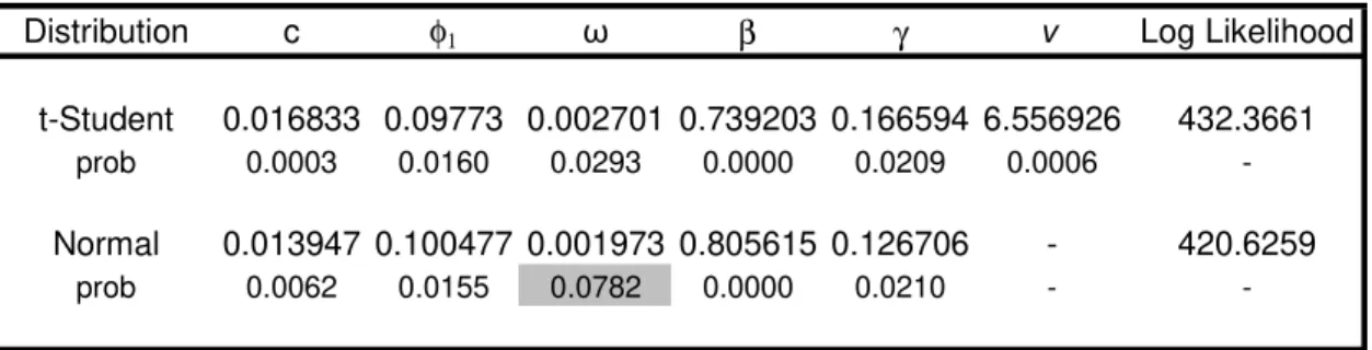
Table 3 - Parameters Estimated for Normal distribuiton and for t-Student distribuiton

Distribution c φ1 ω β γ ν Log Likelihood

t-Student 0.016833 0.09773 0.002701 0.739203 0.166594 6.556926 432.3661

prob 0.0003 0.0160 0.0293 0.0000 0.0209 0.0006

-Normal 0.013947 0.100477 0.001973 0.805615 0.126706 - 420.6259

prob 0.0062 0.0155 0.0782 0.0000 0.0210 -

-The estimated parameters, obtained by Eviews, for normal and t-student

distribution are presented on table 3 above. The model is well specified using

GJR-GARCH model combined with T-Student distribution all estimated coefficients are

statistically significantly. For normal distribution one of the GARCH parameters is

(34)

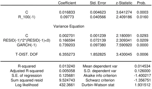
4. Estimation Results

Considering the particular GJR-GARCH model and the t-Student distribution, the

final model results are presented on table 4 below. The modelling estimation was achieved

by Eviews,

Table 4 - TGARCH Model EVIEWS Output

Dependent Variable: R_100

Method: ML - ARCH (Marquardt) - Student's t distribution Sample (adjusted): 2 610

Coefficient Std. Error z-Statistic Prob.

C 0.016833 0.004623 3.641274 0.0003

R_100(-1) 0.09773 0.040566 2.409186 0.0160

Variance Equation

C 0.002701 0.001239 2.180091 0.0293

RESID(-1)^2*(RESID(-1)<0) 0.166594 0.072139 2.309341 0.0209

GARCH(-1) 0.739203 0.097380 7.590920 0.0000

T-DIST. DOF 6.355273 1.852825 3.430045 0.0006

R-squared 0.013240 Mean dependent var 0.014534 Adjusted R-squared 0.005058 S.D. dependent var 0.126000 S.E. of regression 0.125681 Akaike info criterion -1.400217 Sum squared resid 9.524743 Schwarz criterion -1.356751 Log likelihood 432.3661 Durbin-Watson stat 1.931512

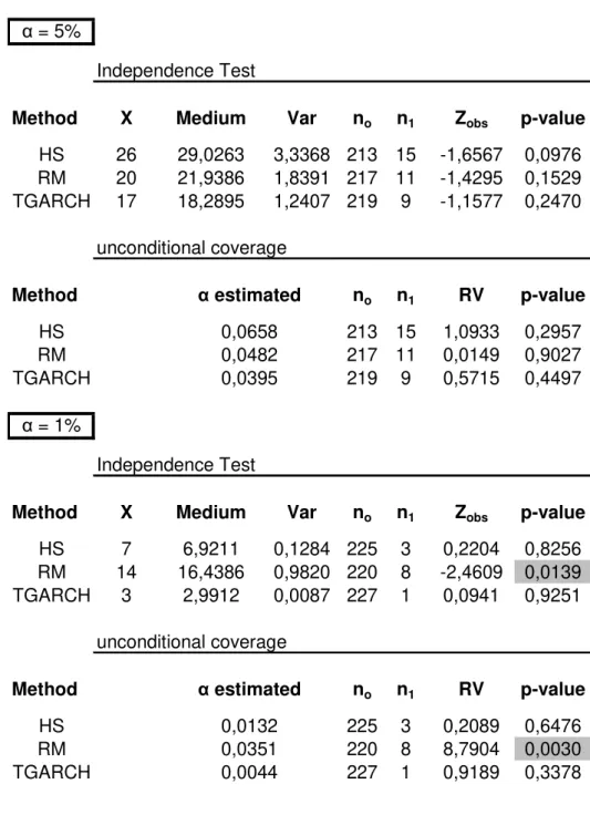
The Backtesting methodology was applied analysing all history returns from the

beginning of 2006. The Backtesting results for one holding period, for both confidence

(35)

α = 5%

Independence Test

Method X Medium Var n_o n₁ Z_obs p-value

HS 26 29,0263 3,3368 213 15 -1,6567 0,0976

RM 20 21,9386 1,8391 217 11 -1,4295 0,1529

TGARCH 17 18,2895 1,2407 219 9 -1,1577 0,2470

unconditional coverage

Method n_o n₁ RV p-value

HS 213 15 1,0933 0,2957

RM 217 11 0,0149 0,9027

TGARCH 219 9 0,5715 0,4497

α = 1%

Independence Test

Method X Medium Var no n1 Zobs p-value

HS 7 6,9211 0,1284 225 3 0,2204 0,8256

RM 14 16,4386 0,9820 220 8 -2,4609 0,0139

TGARCH 3 2,9912 0,0087 227 1 0,0941 0,9251

Method no n1 RV p-value

HS 225 3 0,2089 0,6476

RM 220 8 8,7904 0,0030

TGARCH 0,0044 227 1 0,9189 0,3378

Table 5 - Backtesting results for one holdind period

0,0482

0,0351 0,0395 α estimated

0,0658

α estimated 0,0132

For one holding period and for a 1% confidence level, the RiskMestrics does not

(36)

α = 5%

Independence Test

HS 5 21,9196 1,8687 213 11 -12,3773 0

RM 10 23,7143 2,2118 212 12 -9,2215 0

TGARCH 12 25,4911 2,5799 211 13 -8,3993 0

HS 213 11 0,0038 0,9510

RM 212 12 0,0588 0,8083

TGARCH 211 13 0,2902 0,5901

α = 1%

Independence Test

HS 7 14,5625 0,764 217 7 -8,6519 0

RM 5 8,8571 0,2416 220 4 -7,8472 4E-15

TGARCH 7 16,4286 0,9983 216 8 -9,4368 0

HS 217 7 6,5350 0,0106

RM 220 4 1,1326 0,2872

TGARCH 0,0357 216 8 8,9984 0,0027

Table 6 - Backtesting results for one week holdind period

0,0536

0,0179 0,0580 α estimated

0,0491

α estimated 0,0313

As referred, under the literature, VaR is generally calculated for different periods of

(37)

next five and ten holding periods, i.e., one week and two weeks. The results are present

on table 6 for one-week holding period above, and on table 7 below for two weeks holding.

α = 5%

Independence Test

Method X Medium Var n_o n₁ Z_obs p-value

HS 9 21,8950 1,9069 208 11 -9,3380 0

RM 5 16,4155 1,0194 211 8 -11,3065 0

TGARCH 13 27,2100 3,031 205 14 -8,1621 0

HS 208 11 0,0002 0,9876

RM 211 8 0,9193 0,3377

TGARCH 205 14 0,8250 0,3637

α = 1%

Independence Test

HS 3 14,5525 0,7804 212 7 -13,0780 0

RM 3 6,9178 0,1335 216 3 -10,7227 0

TGARCH 3 12,6712 0,5713 213 6 -12,7951 0

HS 212 7 0,0002 0,9876

RM 216 3 0,27129 0,3377

TGARCH 0,0274 213 6 4,5416 0,0331

Table 7 - Backtesting results for two weeks holdind period

0,0365 0,0639 α estimated

0,0502

α estimated 0,0320 0,0137

As the periods are getting higher the independence is being lost. For the three

(38)

volatilities are not good VaR measures. Forecasted volatilities do not have the property of,

the sequence of the events exceeding VaR behaves like an i.i.d..

5. Main Findings

The main objective of this study was to evaluate and analyse forecasted volatilities as

good VaR estimators for a Financial Institution portfolio.

Through the use of three different methodologies for two different confidence levels

and for three time holding periods, backtests were performed in order to achieve the main

conclusions.

The backtests reveal that volatilities are good VaR measures for one holding period

under the parametric technique AR(1)+GJR-GARCH for both confidence levels, and as

well for the non parametric technique – Historical Simulation. RiskMetrics, the other

parametric technique, turned out to be a good VaR measure only for one holding period at

a 5% confidence level. For the other two holding periods forecasted volatilities revealed

not to be good VaR measures.

The final figures for Value-at-Risk, for one holding period and for 95% confidence level

(39)

VaR 1

Table 8 - Value-at-Risk for one day holding period, 5% confidence level

Pn

α=5% Historical TGARCH

Simulation RiskMetrics

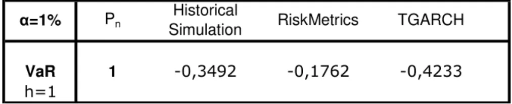
On table 9 below, the final figures for Value-at-Risk for one holding period for 1%

confidence level are presented.

VaR 1

Table 9 - Value-at-Risk for one day holding period, 1% confidence level

TGARCH

α=1% P_n Historical

Simulation RiskMetrics

The well-known shortcoming, under the literature, on the non-parametric technique

Historical Simulations it is the fact does not grab the dynamic of the conditional variance.

The changes in the risk portfolio are associated only with the historical experience of the

portfolio, and the quantiles rest on the assumption that any return in a particular period is

equally likely.

Under the limitations of RiskMetrics methodology, referring it underestimates VaR due

to the normality assumption that generally is not consistent with the general behaviour of

financial data, the GJR-GARCH methodology reveals to be the most accurate measure to

(40)

For further developments it would be interesting to evaluate other confidences levels,

less than 1%, and estimating VaR through the use of semiparametric techniques such as

(41)

References

Ahlgrim, K. and Candidate, P. (1999), Investigating the use of Value-at-Risk in Insurance, working paper, University of Illinois at Urbana-Champaign, Department of Finance.

Angelidis, T., Benos, A. and Degiannakis, S. (2004), The use of Garch Models in VaR Estimation, statistical methodology, vol.1, pp. 105-128.

Artzner, P. (1999), Application of Coherent Risk Measures to Capital Requirements in Insurance, North American Actuarial, Vol. 2, n.2, pp. 11-25.

Basel Committee on Banking Supervision (2001), Consultative Document: The internal Ratings-Based Approach, Bank for International Settlements.

Black, F. (1976), Studies of Stock Market Volatility Changes, in: Proceedings of the American Statistical Association, Business and Economic Statistic Section, pp. 177-181.

Bollerslev, T. (1986), GARCH, Journal of Econometrics, 31, pp. 307-327.

Campbell, Y. Lo, W. and Craig, A. (1997), The Econometrics of Financial Markets, Princeton University Press.

Christoffersen, P., Diebold and Schermann, T. (1998), Horizon Problems and Extreme events in Financial Risk Management, Economic Policy Review, New York:Federal reserve Bank of New York, pp. 109-118.

Christoffersen, P., Hahn, J. and Inoue, A. (2001), Testing and Comparing Value-at-Risk Measures, Journal of Empirical Finance, vol. 8, pp. 325-342.

Danielson, J. and Vries, C. G. (1997), Value at Risk and Extreme Returns, Manuscript, London School of Economics.

Dimson, E., Marsh, P. (1995), Capital Requirements for Securities Firm, Journal of Finance, vol 50 pp.821-851.

(42)

Duffie, D. and Pan, J. (1997), An overview of Value at Risk. The Journal of Derivatives, pp. 7-49.

Embrechts, P. (1998), Extreme value theory as a Risk Management Tool, North American Actuarial Journal, 3 (2), pp. 30-41.

Engle, R. (1982), Autoregressive Conditional Heteroscedasticity with Estimates of the Variance of United Kingdom Inflation, Econometria, vol. 50, pp. 987-1007.

Giannopoulos, K. (2002), VaR modelling on long run horizons, Risks in Economics and Financing, translated from Automatik i Telemekhanika, n.º 7, pp. 87-93.

Glosten, L., Jagannathan, R. and Runkle, D. (1993), On the Relation Between the expected Value and the Volatility of the nominal excess return on stocks, Journal of Finance, 487, pp. 1779-1801.

Jorion, P. (1997), Value at Risk: The New Benchmark for Controlling Market Risk, MCGraw Hill.

J.P. Morgan (1996), Risk MetricsTM-Technical Document, Fourth edition, New York: Morgan Guaranty Trust Company.

Lauridsen, S. (2000), Estimation of Value at Risk by Extreme Value Methods, Klumer Academic Publishers Extremes, 3:2, pp. 107-144.

Manganelli, S. and Engle, R. (2001), Value at Risk Models in Finance, Working Paper n.75, European Central Bank.

McNeil, A. and Frey, M. (2000), Estimation of Tail-Related Risk measures for Heteroscedastic Financial Series: An Extreme Value Approach, Journal of Empirical Finance, 7, pp. 271-300.

Newbold, P., Carlson, W. and Thorne, B. (2003), Statistics for Business and Economics, fifth edition, New Jersey: Prentice Hall

(43)

Sarma, M., Thomas, S. and Shah, A. (2003), Selection of Vale-at-Risk Models, Journal of Forecasting, vol. 22, pp. 337-358.

Sousa, L. (1999), Valor em Risco em épocas de Crise, Master Dissertation, Brasil: Universidade São Paulo - Faculdade de Economia e Administração Fiscal.

Swiss Reinsurance Company (2006), Sigma n.º4/2006- Solvency II: an Integrated approach, Economic Reasearch&Consulting, http://www.swissre.com/, pp.3-44.

Wagster, J. (1996), Impact of the 1988 Basle Accord on Internacional Banks, Journal of Finance, vol 51, pp. 1321-1346.

Wirch, J. (1999), A Synthesis of Risk Measures for Capital Adequacy, Insurance: Mathematics and Economics, Vol. 25, n. 3, pp. 337-347.

(44)

Appendix*

Programming Code – AR(1)+TGARCH, one, five and ten holding periods, indicator backtesting library cml,util,pgraph,est_etd,testes;

cls;

y = SpreadsheetReadM("dados rc", "d3:d612",1 ); y=y*100;

n=rows(y); @ k=290; @ k=382; alfa=.05; missing={.};

Value_at_Risk=missing*ones(rows(y),1); Indicador=missing*ones(rows(y),1); controle={};

h=1; \* h=5 ; h=10 */

b0=0.11889583|0.014438678|0.0027099201|0.15353301|0.74367327|7;\* Vector Inicial MV */ for i (k,n-h,1);

{b,f0,grad,cov,retcode}=tStudent_garch_Sandra(b0,y[1:i]); if retcode /= 0;

controle =controle|i; endif;

b0=b;

m=b[1]*y[i]; /* media*/

m=(y[i]*(-1 + b[1])*b[1]*(-1 + b[1]^h) +

b[2]*(h - h*b[1] + b[1]*(-1 + b[1]^h)))/(-1 + b[1])^2;

u=y[i]-m; /* erro*/

v_1=b[3]+b[4]*(u < 0)*u^2+b[5]*var[rows(var)]; /* variancia a um passo*/ v_h=-((h*b[3] + (b[1]*(-1 + b[1]^h)*(-2 - b[1] + b[1]^(1 + h))*b[3])/(-1 + b[1]^2) +

v_1*(1 - (b[4]/2 + b[5])^h) + (b[3] -

b[3]*(b[4]/2 + b[5])^h)/(-1 + b[4]/2 + b[5]) + (b[3] + v_1*(-1 + b[4]/2 +

b[5]))*((b[

1]^(2 + 2*h)*(-1 + ((b[4]/2 + b[5])/b[1]^2)^h))/(b[ 1]^2 - b[4]/2 - b[5]) - (2*

b[1]^(1 + h)*(-1 + ((b[4]/2 + b[5])/b[1])^h))/(b[1] -

b[4]/2 - b[5])))/((-1 + b[1])^2*(-1 + b[4]/2 + b[5]))); /* variancia a h passos*/

quantil=cdfni(alfa); /* quantil normal */ Value_at_Risk[i+h]=-(m+quantil*sqrt(v_h)); if sumc(y[i+1:i+h]) < -Value_at_Risk[i+h]; indicador[i+h]=1;

else;

indicador[i+h]=0; endif;

endfor;

print "controle";; controle; i=packr(indicador);

(45)