Goog
le
Search
Vo
lume
as
a
proxy
o
f
Investor
Attent
ion:
are
prev
ious
f
ind
ings
robust?
João
Tan
issa
Pancada
D
issertat
ion
wr
itten
under
the
superv
is
ion
o
f
Bruno
Gerard
D
issertat
ion
subm
itted
in
part
ia
l
fu
l
f
i
lment
o
f
requ
irements
for
the
MSc
in
F
inance
,
at
Un
ivers
idade
Cató
l
ica
Portuguesa
and
for
the
MSc
in
F
inanc
ia
l
Abstract
I assess the robustness to different periods and panel models of several findings in the literature that uses Google search volume as an investor attention proxy. With all S&P 500 stocks between 2004 and 2016, I confirm that weekly search volume is persistent and increases are associated with high share turnover as well as earnings announcements. When the CCEMG estimator of Pesaran (2006) is used, I find evidence against Da et al. (2011) but consistent with Barber and Odean (2008). Even for large stocks, surges in people’s attention predict positive abnormal returns one week ahead, which reverse within one year. I conclude the literature should adopt panel estimators more robust to the presence of both firm and time effects.
Resumo
Eu avalio a robustez em diferentes períodos e modelos em painel de várias conclusões na literatura que usa o volume de pesquisa no Google para medir a atenção dos investidores. Com todas as ações do S&P 500 entre 2004 e 2016, eu confirmo que o volume de pesquisa semanal é persistente e aumentos estão associados a um alto volume de transações de ações assim como à divulgação de resultados. Quando o estimador CCEMG de Pesaran (2006) é utilizado, eu encontro evidência contra Da et al. (2011) mas consistente com Barber e Odean (2008). Mesmo para grandes empresas, aumentos na atenção das pessoas preveem retornos anormais positivos na semana seguinte, que invertem dentro de um ano. Eu concluo que a literatura deveria adotar estimadores em painel mais robustos à presença de efeitos quer de tempo quer de empresa.
Acknowledgments
I would like to thank several people that contributed directly or indirectly to the success of this thesis. First of all, I am glad that Professor Bruno Gerard accepted to be my supervisor. His prompt feedback and guidance were very helpful. I would have gone much further with his advice had I started earlier. Secondly, the unconditional support of my family throughout the process was crucial to finish the thesis on time. A special thanks goes to my brother, whose programming skills were vital to obtain the key variable of this thesis (Google search volume). Thirdly, I appreciate the comments and suggestions of many Statalist users to my econometric and Stata related doubts. In addition, I am thankful to several researchers whose Stata code I extensively used. Finally, I would like to thank Google Inc. for making available a measure of their historical search volume, which has sparked substantial research in many different fields.
Table of Contents
1. Introduction _____________________________________________________________ 1 1.1 Motivation ____________________________________________________________ 1 1.2 Google Search Volume as a demand proxy __________________________________ 2 1.3 Research problem and thesis contribution ___________________________________ 4 2. Literature Review ________________________________________________________ 6
2.1 Investor attention and its impact on financial markets __________________________ 6 2.2 Traditional proxies of investor attention _____________________________________ 7 2.3 Demand proxies of investor attention _______________________________________ 8 2.4 Google Search Volume __________________________________________________ 9 3. Methodology ___________________________________________________________ 10
3.1 Panel regressions - background ___________________________________________ 11 3.2 Panel regressions with varying intercepts ___________________________________ 12 3.3 Factor-augmented regressions ____________________________________________ 14 3.4 Dynamic panel regressions ______________________________________________ 15 4. Data ___________________________________________________________________ 16
4.1 Sample construction ___________________________________________________ 16 4.2 Google Search Volume _________________________________________________ 19 4.3 Other major variables __________________________________________________ 20 4.4 Summary statistics and correlations _______________________________________ 21 4.5 Univariate tests _______________________________________________________ 24 5. Results and Analysis _____________________________________________________ 26
5.1 Hypothesis 1 _________________________________________________________ 26 5.2 Hypothesis 2 _________________________________________________________ 29 5.3 Hypothesis 3 _________________________________________________________ 32 6. Conclusion and Future Research ___________________________________________ 35 References _______________________________________________________________ 37 Appendix A – Google Search Volume _________________________________________ 44 Appendix B – Stata User-Written Commands __________________________________ 45 Appendix C – Robustness Analysis ___________________________________________ 46
Index of Figures and Tables
Figure 1. Illustration of Google Trends Ouput _________________________ 3 Table 1. Variables Definition ______________________________________ 17 Table 2. Summary Statistics _______________________________________ 22 Table 3. Correlation Matrix _______________________________________ 23 Table 4. Univariate Tests _________________________________________ 25 Table 5. ASVI as a function of existing Attention Proxies _______________ 27 Table 6. ASVI and Retail Investor Attention _________________________ 31 Table 7. ASVI and Future Abnormal Returns ________________________ 34 Table C.1 Hypothesis 1: Robustness Analysis _________________________ 46 Table C.2 Hypothesis 2: Robustness Analysis _________________________ 49 Table C.3 Hypothesis 3: Robustness Analysis _________________________ 51
1. Introduction
1.1 Motivation
We are currently living in the information age. The Internet, and subsequent innovations, have allowed a myriad of news and data to spread very fast and at a low cost across the world (Rubin and Rubin, 2010). Investors should not miss this constant information flow, since financial markets are known to be sensitive to new information (French and Roll, 1986). In the limit, as traditional asset pricing models assume, security prices reflect all available information, with new one being immediately incorporated once it is made public (Merton, 1987).
However, there is only so much information people can process each day. It takes time to obtain and then decide how to act on new data. Consequently, investors have to be selective and traditional models fail to consider these limitations (Peng and Xiong, 2006). Inattention can significantly impact asset prices and compromise market efficiency as the adjustment to new information takes longer than expected. For instance, Huberman and Regev (2001) take the extreme example of EntreMed, a US biotech company whose stock price soared 330% in one day. This rise followed a news piece from the New York Times on a research breakthrough that had been featured on Nature magazine 6 months before.
Measuring investor attention (or distraction) is no easy task. It is difficult to quantify the effort people put into, for example, collecting data or reading the news on a given company. Simply asking people is not a feasible strategy. Therefore, rather than looking at the demand for information, the literature has traditionally focused on indirect proxies that fit in one of two categories (Vlastakis and Markellos, 2012): a) supply side of information – e.g., Lou (2014) for advertising expenditures and Yuan (2015) for front-page articles; b) market data – e.g., Barber and Odean (2008) for abnormal turnover and extreme returns.
Nevertheless, as some (proprietary) databases are made public, there is a relatively recent trend that uses demand proxies. Starting with internet blogs (e.g., Antweiler and Frank, 2004), researchers have been trying to capture people’s attention through their online behaviour. Once their actions or interests are revealed, an analogy to the concept of revealed preferences in microeconomics, we are one step closer towards measuring people’s effort.
1.2 Google Search Volume as a demand proxy
One way of assessing the interests of many individuals at a point in time is to know what they search on Google. Ginsberg et al. (2009) are among the first to document the usefulness of Google’s Search Volume Index (hereafter SVI) by showing that it can detect influenza outbreaks. Shortly after, Da et al. (2011) introduced SVI as a measure of aggregate investor attention in the US. They found it captures well retail activity and that high values help predict abnormal returns.
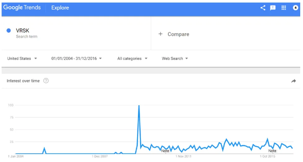
SVI is available to the general public through Google Trends since May 2006, but the database starts in 2004 (https://trends.google.com). When we type a set of words or ‘search terms’ into Google Trends, the platform returns a relative measure of their search volume history. To illustrate, monthly SVI is plotted for the term ‘VRSK’ in figure 1. It is based on searches from Google web users in the US during January 2004 to December 2016. ‘VRSK’ stands for the stock ticker of Verisk Analytics, a US data analytics company. Each monthly observation represents the ratio of search volume on ‘VRSK’ over the search volume on all terms in the US that month, scaled by the maximum monthly ratio from 2004 to 20161. We can
see there is practically no interest on that term prior to October 2009 but, suddenly, there is a search pattern that fluctuates over time. This is not a coincidence because the peak on that date represents the company’s IPO month. Therefore, the word ‘VRSK’ gained a distinctive meaning after October 2009 and people started typing it regularly. This is clear evidence that SVI can capture people’s attention.
With the example of figure 1 in mind, there are two reasons to believe that aggregate search data from Google can be a good attention proxy. First, search frequency directly reveals whether people are interested in certain events (or companies) over time. This requires, however, that we specify the search term that (potential) investors often use. As discussed in section 4.2, I use each stock’s ticker symbol. Second, Google continues to dominate the US market for web search engines, with a share fluctuating between 59% and 69% from 2008 to 20162. Therefore,
it is expected that Google searches represent the general search behaviour in the US.
1 See section 1 of appendix A for a more detailed explanation of this two-step process.
2 Source: Statista -
Figure 1. Illustration of Google Trends Ouput
This figure shows the top half of the output from Google Trends when typing the term ‘VRSK’ on September 10th 2017. From January 2004 to December 2016, the chart plots monthly SVI for Google web searches on that term in the US. The series ranges from 0 to 100. Each monthly observation represents the ratio of search volume on ‘VRSK’ over the search volume on all terms in the US that month, scaled by the maximum monthly ratio from 2004 to 2016. See section 1 of appendix A for a more detailed explanation of how to interpret SVI. The notes that appear above the horizontal axis simply indicate two (out of many other) dates when the system was improved.
1.3 Research problem and thesis contribution
The aim of this thesis is to examine in detail the consistency of several findings in the SVI literature to more recent time periods and robust panel estimators. This is done by testing the following three hypothesis:
1. Is SVI related but different from existing investor attention proxies? Hypothesis 1:SVI is similar to existing proxies of investor attention.
2. Does SVI mainly capture the attention of retail investors?
Hypothesis 2:SVI does not capture the search behaviour of retail investors. 3. Is SVI in favour of the findings of Barber and Odean (2008)?
Hypothesis 3:SVI does not predict positive returns in the short-term for large stocks, which reverse within a year.
Using all stocks that were ever part of the S&P 500 index between 2004 and 2016, the contribution of this thesis is twofold. I am the first testing hypothesis 1 under a new method of computing SVI and with 13 rather than 4 to 5 years of weekly data as in Da et al. (2011) and Drake et al. (2012). The same essentially applies to hypothesis 3 because Cziraki et al. (2017) use a lower frequency (i.e. monthly data) and do not entirely follow the method of Da et al. (2011).
The second contribution concerns a more rigorous econometric treatment of the underlying panel data. Recent research has shown that parameter consistency of standard methods can be significantly affected in the presence of cross-sectional dependence (e.g., Hjalmarsson, 2010; Graevenitz et al., 2016; Westerlund et al., 2017). The literature on SVI, and on investor attention in general, has greatly overlooked this issue. When testing hypothesis 1, researchers have simply used pooled OLS with time dummies and adjusted standard errors. Even Fama-MacBeth (1973) regressions, used by Da et al. (2011) and Cziraki et al. (2017) in hypothesis 3, may be problematic (e.g., Campello et al., 2013). I argue we should rather apply the CCEMG model of Pesaran (2006) because of the high cross-sectional dependence that is expected in financial data (Philipps and Moon, 1999; Pesaran, 2007). Finally, I suspect that the persistency of Google search, as seen in the VAR model of Da et al. (2011), might also be important to take into account, even in static models.
Overall, results indicate that the three hypothesis are rejected and it is very important to consider the structure of the data as well as different time periods.
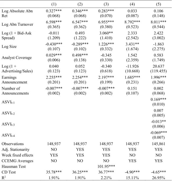
In hypothesis 1, I do find that SVI is capturing a quite unique phenomenon as in Da et al. (2011) and Drake et al. (2012). However, in more recent periods, the explanatory power of existing attention proxies can be more than twice of what was previously assumed. Furthermore, only two proxies keep their anticipated relation with Google search over time. There is strong evidence that SVI increases when trading volume is high and when a company announces its quarterly earnings. This is also very good news about the usefulness of SVI as an attention proxy.
I also find that Google search is a persistent variable up to its 4th lag. Even though these
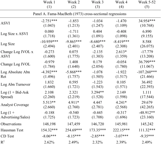
lags appear to be correlated with the regressors, their omission does not materially influence the results. Non-stationarity is also not a major concern, but I find that it is essential to consider firm effects and cross-sectional dependence. In hypothesis 1, variables such as analyst coverage, the bid-ask spread, and absolute abnormal returns become statistically insignificant when more robust models are used. Most importantly, in hypothesis 3, the main conclusions dramatically change with the CCEMG estimator. I show that current week abnormal SVI predicts positive abnormal returns next week, which reverse within one year. This is robust to different time periods and ways of computing abnormal SVI. When ‘noisy’ tickers are removed, the effect is even stronger. The opposite conclusion, the one documented in Da et al. (2011), is found when using Fama-MacBeth (1973) regressions. Therefore, I support the predictions of Barber and Odean (2008) for large stocks.
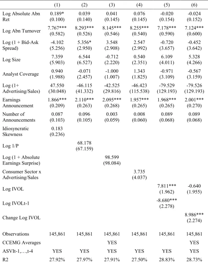
Nevertheless, I confirm that SVI’s effect is stronger among smaller stocks, as in Da et al. (2011), but not for those that retail investors are more likely to trade. In hypothesis 2, the change in idiosyncratic volatility is the only retail activity proxy that has a consistent positive relation with abnormal SVI over time. However, it is not robust against aggregate abnormal returns, which is expected given its indirect nature. The conclusion might change with a proprietary database on retail activity such as NYSE ReTrac, but that is left for future research.
This thesis proceeds as follows. Section 2 provides an overview of the background literature. Section 3 explains the methodology and section 4 describes the data. Section 5 explains each of the three hypothesis in detail and examines the results. Section 6 concludes and discusses where future research can be useful.
2. Literature Review
This section starts with the fact that investor attention is limited and it can affect financial markets. Traditional and demand proxies of attention are then outlined. This section finishes with an emphasis on the demand proxy used in this thesis, which is Google’s Search Volume Index.
2.1 Investor attention and its impact on financial markets
The tradition in financial economics has been to assume that people act rationally in their investment decisions so that their utility is always maximized (Barber and Odean, 2011). This requires that investors keep analyzing the risk-return trade-off of all assets until they find their optimal portfolio, given their level of risk aversion. Under the Capital Asset Pricing Model of Sharpe (1964) and Lintner (1965), arguably the most famous model in asset pricing, all investors end up holding the same well-diversified portfolio of risky assets, which is the market portfolio. When new information is released to the public, and there are no frictions, prices react immediately as investors revise their risk-return expectations.
In reality, the adjustment may take time because frictions abound. One of the most pervasive is intrinsic to human nature, namely our limited cognitive resources (Kahneman, 1973). There are thousands of investment opportunities available and new information is being constantly produced about them. However, people do not have the time or the capacity to process and incorporate all that information in their investment decisions (e.g., Hirshleifer and Teoh, 2003; Peng, 2005).
Merton (1987) is the first to formally recognize the importance of investor attention in financial markets and to theorize its implications. His main contribution is that a firm’s market value is increasing with investor recognition but expected returns are decreasing. The impact of a larger investor base has been validated empirically by Kadlec and McConnell (1994) and Chen et al. (2004), among others.
In a growing literature, other predictions have been proposed. For example, Peng and Xiong (2006) and Mondria (2010) postulate that limited attention leads people to act more on general signals (market or sector) rather than firm-specific, which increases stock co-movement. Hou et al. (2009) argue that the post-earnings announcement drift and the momentum anomaly are due to, respectively, investor underreaction and overreaction to information. Nieuwerburgh and Veldkamp (2010) suggest that when investors have to choose which information to collect before investing, their portfolio allocation is sub-optimally diversified.
Since it is clear that investor attention is limited, the next question is: where do investors focus their attention? The literature seems to be unanimous in that investors’ attention is directed towards familiar or ‘attention-grabbing’ stocks. Seasholes and Wu (2007) find that investors are induced to buying stocks they did not own when prices hit upper limits on the Shanghai Stock Exchange. Likewise, Barber and Odean (2008) show that retail investors are net buyers of stocks that have recently caught their attention after periods of abnormal returns, turnover and news coverage. Corwin and Coughenour (2008) study NYSE’s specialists and argue that these market makers dedicate more effort to their most active stocks, leading to less liquidity in the other securities they trade. Others have argued that limited attention leads investors to prefer the stock of domestic companies and of their employer, which can help explain the home bias puzzle (e.g., Coval and Moskowitz, 1999; Huberman, 2001).
The common issue among these researchers is that they can only provide indirect evidence of limited attention, since this is something difficult to measure or observe (Corwin and Coughenour, 2008). Based on Vlastakis and Markellos (2012), proxies of attention can be divided into three distinct groups: market data, supply of information, and information demand. The former two have been the tradition in the literature due to data limitations and are discussed in the next section. The latter, where SVI is included, has seen tremendous growth in recent years and is explored in sections 2.3 and 2.4.
2.2 Traditional proxies of investor attention
There is a vast literature of indirect proxies measuring investor attention. On the supply side of information, the two most popular measures have been news coverage and advertising expenditures. The reason is that both are associated with higher company visibility to the public, and hence to investors. The results are in general consistent with the predictions of Merton (1987).
The study of Thompson et al. (1987) is one of the first to document that both firm returns and their volatility change when firm-specific news are published on the Wall Street Journal. More recently, Ryan and Taffler (2004) present evidence that corporate news are important drivers of price changes and trading volume in the London Stock Exchange. Fang and Peress (2009) find in the cross-section that companies with no media coverage earn a return premium even after controlling for 5 common risk factors. Their results are stronger among smaller stocks and for companies with low analyst coverage, high idiosyncratic volatility, and high retail investor ownership. The importance of the media remains whether researchers take into
account the content of news articles (e.g., Mitchel and Mulherin, 1994; Tetlock, 2007) or focus on the impact of market-wide news (e.g., Berry and Howe, 1994).
Grullon et al. (2004) and Frieder and Subrahmanyam (2005) show that more product advertising increases the number of individual and institutional investors. Chemmanur and Yan (2009) find that firms increase their levels of advertising when they aim at issuing equity. This spillover to the financial markets is found by Lou (2014) to have a temporary positive effect on returns due to retail investors. In turn, the researcher argues this is opportunistically considered by firm executives to either sell their company stock, issue new equity or finance acquisitions with stock.
In terms of market proxies, examples abound. Absolute and extreme stock returns have been used, respectively, by Corwin and Coughenour (2008) and Barber and Odean (2008). The drivers of high returns may catch investor attention as well as high returns themselves. Periods of high trading volume are also likely to be associated with higher investor interest (e.g., Gervais et al., 2001; Hou et al., 2009). When several firms announce their earnings at the same time, investors might not be able to follow all of them, which results in underreaction to the new information (e.g., Hirshleifer et al., 2009; Drake et al., 2012). Analyst coverage and stock liquidity have also been used (e.g., Da et al., 2011; Drake et al., 2012). The reason is that a company with more analysts and a more liquid stock is likely to have less information asymmetry. Therefore, investors do not need to spend as much effort processing company related information (Arbel, 1985; Leuz and Verrecchia, 2000).
2.3 Demand proxies of investor attention
The relevance of information demand was already well recognized in the theoretical literature (e.g., Kihlstrom, 1974; Grossman and Stiglitz, 1980). However, it was only possible to study this ‘new class’ of proxies with the advent of the internet and the subsequent release of proprietary data. Demand proxies are currently obtained from two different sources: online posting activity (e.g., internet forums, social media) and search volume (e.g., Google, Baidu).
Using more than 1.5 million posts from Raging Bull and Yahoo! Finance, Antweiler and Frank (2004) find intra-day and one day predictability for stock trading volume and volatility but not for returns. Das and Chen (2007) also do not find evidence for returns using Yahoo! messages. Later, Rubin and Rubin (2010) turned to the editing frequency of Wikipedia articles. They present evidence in favour of a positive relation where higher editing is associated with lower earnings surprises and less dispersion in analysts’ forecasts.
With the emergence of social media, researchers started developing larger scale algorithms3.
Bollen et al. (2011) show that daily mood changes on Twitter posts are correlated with changes in the DJIA Index over the next days. Siganos et al. (2014) use Facebook’s sentiment index and find evidence that there is a positive contemporaneous relation between sentiment and stock market returns, which then reverses in the following weeks. Chen et al. (2014) analyse an exclusively investment-related website (Seeking Alpha). Using more companies and a longer period than previous studies, they show that people’s opinions help predict future stock returns and anticipate earnings surprises.
The importance of studying investors’ search patterns is motivated by the marketing literature. It is well-known that consumers spend (more or less) time searching for alternatives and understanding product features before making a purchase (e.g., Beatty and Smith, 1987). Thus, investor search can be considered a leading indicator of their investment decisions (Choi and Varian, 2009).
Mondria et al. (2010) started the finance literature on web search engines using AOL and link the US home bias to investor attention. Preis et al. (2010) and Da et al. (2010, 2011) followed with Google search volume, as discussed in the next section. Shi et al. (2012) use data from Baidu search engine and reach similar results as Barber and Odean (2008). Drake et al. (2015) use SEC’s EDGAR search traffic and find that information demand is positively related to several corporate events. Lawrence et al. (2016) use Yahoo! Finance and show companies in the highest quintile of abnormal search outperform those at the bottom, an effect that has no reversal even after 1 year. The most recent contribution is that of Ben-Rephael et al. (2017), who for the first time directly study the behaviour of institutional investors through their searches on Bloomberg Terminal. They find that only retail investors are distracted by many news on the same day and firm-specific news, rather than market-wide information as suggested by Peng and Xiong (2006), are the relevant firm drivers for institutional investors.
2.4 Google Search Volume
Google Trends was launched on May 2006 and Google Insights on August 20084. Initial
studies have used Google search to anticipate widespread diseases (e.g., Ginsberg et al., 2009),
3Practitioners have incorporated such algorithms in their trading strategies using Twitter.
Source: Business Insider - http://www.businessinsider.com/sell-signal-hedge-fund-unveils-secret-weapon-to-beat-the-market-twitter-2011-5 (retrieved on September 20th, 2017).
4 They were merged in 2012 and the method of Insights is now the one of Google Trends. It used to be just the
forecast unemployment claims (e.g., Askitas and Zimmermann, 2009) and private consumption (e.g., Choi and Varian, 2009).
The finance literature on SVI started with Preis et al. (2010), who find a positive correlation between changes in web search and trading volume for S&P 500 stocks. Several other papers document the same positive relation for individual companies and stock indices as well as with liquidity and volatility (e.g., Bank et al., 2011; Vlastakis and Markellos, 2012; Latoeiro et al., 2013; Andrei and Hasler, 2015). Vlastakis and Markellos (2012) are able to empirically show for the first time that information demand, given by Google searches, increases with the variance risk premium, which is proxying for the level of investor risk aversion.
Nevertheless, the most influential findings are those found in a series of papers from Da, Engelberg, and Gao, who use a comprehensive dataset of Russell 3000 stocks. Da et al. (2010) show that the momentum effect is stronger among the most searched stocks, especially for those in the winner’s portfolio. They argue that occurs because SVI is capturing the attention of retail investors. This hypothesis is successfully tested in Da et al. (2011) and Gwilym et al. (2016). In addition, Da et al. (2011) and Drake et al. (2012) show that existing proxies of attention explain little variation in Google search, with reported regression R2 below 4%.
In terms of stock returns, several papers predict a positive relation with SVI in the short-term (e.g., Da et al., 2011; Bank et al., 2011; Joseph et al., 2011; Gwilym et al., 2016), including for stock markets (e.g., Da et al., 2014; Vozlyublennaia, 2014). The effect starts reversing after four or five weeks, which is consistent with investor sentiment predictions described in section 2.3. In fact, Da et al. (2014) builds a new investment sentiment index based on Google searches. However, this relation with returns seems to be only present among small stocks (Da et al., 2011; Bank et al., 2011; Cziraki et al., 2017). Finally, researchers have also shown that SVI increases substantially in the previous and at the same week of important corporate events such as IPOs, earnings announcements, and mergers announcements (Da et al., 2011; Drake et al., 2012; Siganos, 2013).
3. Methodology
The empirical analysis in this thesis is conducted through panel data regressions. Panel analysis is to a large extent a combination of both time-series and cross-sectional analysis (Wooldridge, 2009). The four sections that follow explain step by step the reasoning behind the statistical methods used. I leave to the references their underlying mathematical complexity and, when applicable, to appendix B their corresponding user-written Stata commands.
3.1 Panel regressions - background
In panel data we have two dimensions, firm and time, rather than only firm or time as in, respectively, cross-sectional and time-series analysis. Its great advantage is the ability to more easily solve the omitted variable bias problem (Hsiao, 2014). If the problem does not exist, we may find more efficient estimators than OLS.
When the data on all firms begins and ends at the same dates with no missing observations in between, the panel is said to be balanced. This is not, however, the case here because some firms: a) go bankrupt, b) are delisted after a take-over or merger, 3) only become listed after the sample begins. Having an unbalanced sample is not a major problem by itself because all tests and regressions conducted in this thesis can accommodate that. Based on Cameron and Trivedi (2005), an issue arises if leaving the sample, which is called attrition, is correlated with the regression residuals, i.e., attrition is non-random. This may occur in hypothesis 3 as firms leave the index for reasons related to the dependent variable (stock returns) such as going bankrupt. Section 4.1 outlines a few solutions.
The absolute (and relative) size of both dimensions determine which regression models are used because the asymptotic theory differs. In terms of absolute size, if N is large and T is small, we have the typical case in microeconomics. However, when T becomes large, the time-series properties of the data have to be considered, namely testing for stationarity (Wooldridge, 2009). There is no formal definition of what constitutes large N and T, but several papers that run Monte-Carlo simulations take values between 100 and 200 (e.g., Chudik and Pesaran, 2013; Everaert and Groote, 2016). Therefore, I assume large N and T because my sample (for most regressions) has N = 739 and T̅ = 206. This brings numerous advantages to the traditional fixed T, large N framework. Among others, it allows richer models that can control for cross-sectional dependence but at the cost of dealing with the aforementioned time-series dependence (Baltagi, 2009).
Following Cameron and Trivedi (2005), the most general panel regression is:
𝑦𝑖,𝑡 = 𝑎𝑖,𝑡+ 𝑥𝑖,𝑡 ∗ 𝛽𝑖,𝑡+ 𝑢𝑖,𝑡, i = 1, … , N, t = 1, … . , T, (1) where 𝑦𝑖,𝑡 is the dependent variable, 𝑥𝑖,𝑡 is the vector of regressors, 𝑢𝑖,𝑡 is the error term, i refers
to the firm dimension and t to the time dimension. Equation (1) cannot be estimated because there are far too many parameters as both the intercept (𝑎𝑖,𝑡) and the slope coefficients (𝛽𝑖,𝑡)
vary by firm and over time.
The case of non-constant slopes is not considered in this thesis because: a) both dimensions are large, hence not feasible to estimate all coefficients; b) the interest on SVI has to do with its
applicability in general rather than on any particular firm or time period5. Nevertheless, in most
finance applications, the intercept should not be constant (Petersen, 2009). Therefore, alternatives to the Pooled OLS estimator, which requires constant slopes and intercepts, need to be found.
3.2 Panel regressions with varying intercepts
When the intercept changes by firm and/or over time, but that is not taken into account, the panel model takes the following general form (Bai, 2009):
𝑦𝑖,𝑡 = 𝛼 + 𝑥𝑖,𝑡 ∗ 𝛽 + 𝑢𝑖,𝑡 (2) where 𝑢𝑖,𝑡 = 𝜃𝑖𝐹𝑡+ 𝑣𝑖,𝑡. 𝑣𝑖,𝑡 are individual specific idiosyncratic errors that are assumed iid
and independent of the regressors. 𝜃𝑖 is a vector of factor loadings and 𝐹𝑡 stands for a vector of
unobserved common factors, which can be correlated with the regressors and over time. These last two terms together capture two effects. On the one hand, they consider the impact of time-varying variables that are constant across all firms (called time fixed effects) or heterogeneous such as macroeconomic shocks (Petersen, 2009). On the other hand, they capture firm-specific characteristics that are constant over time (called firm fixed effects) or time-varying such as the accumulation of human capital (Ahn et al., 2013). Time and firm effects have different implications for estimator consistency and valid statistical inference.
In terms of consistency, if these unobserved effects impact the dependent variable but are correlated with some regressors, we have an omitted variable bias. This is likely to occur when testing all hypothesis. For example, time effects such as recessions impact the returns of all firms in different ways (dependent variable of hypothesis 3) but also their advertising expenditures and sales (regressor). Those shocks also impact investor attention, leading more people to search certain companies like Bear Stearns in 2008 (dependent variable in hypothesis 1 and 2).
In terms of inference, the standard errors of the coefficients are underestimated when common factors are not considered, which may give rise to misleading statistical significance (Gow et al., 2010). Thompson (2010) shows that not controlling for time effects leads to cross-sectional error dependence, meaning that the residuals of any two firms are contemporaneously correlated. If these time effects are persistent, then the residuals of different firms at different points in time are also correlated. Finally, not controlling for firm effects leads to serial
5 As far as I know, only Vlastakis and Markellos (2012) in the SVI literature estimate firm-specific regressions,
correlation. However, Thompson (2010) also shows that time and firm effects are only a concern when regressors are themselves, respectively, cross-sectionally correlated and autocorrelated.
The two previous paragraphs motivate the use of regression models that control for both time and firm effects. Traditionally, researches have used the two-way fixed effects model, which is a special case of equation (2) (Pesaran, 2006):
𝑦𝑖,𝑡 = 𝛼 + 𝑥𝑖,𝑡∗ 𝛽 + 𝑢𝑖,𝑡 (3) where 𝑢𝑖,𝑡 = 𝛼𝑖+ 𝛾𝑡+ 𝑣𝑖,𝑡. 𝛼𝑖 stands for firm fixed effects whereas 𝛾𝑡 are time fixed effects.
The former is controlled for by either (quasi) time demeaning the regression or with firm dummies. The latter requires either cross-sectionally demeaning the regression or time dummies.
As argued by Petersen (2009), when the time dimension is smaller than the number of firms, time dummies should be used to control for time fixed effects. Then, we either fully time demean the regression with the fixed effects model or partially do so using the random effects model. The choice depends on whether firm fixed effects cause an omitted variable bias, which can be tested with the robust form of the Hausman test to heteroskedasticity (Wooldridge, 2009). Under the null hypothesis, there is no bias, and the random effects model is more efficient. However, if time or firm effects are not fixed, but they are uncorrelated with the regressors, it is enough to further adjust the standard errors. With large N and T, firm effects are fully corrected when clustering by firm whereas time effects require clustering by time or Fama-Macbeth (1973) regressions (Petersen, 2009).
In section 5, I initially follow the methodology used in the previous literature. For hypothesis 1, Da et al. (2011) and Drake et al. (2012) use Pooled OLS with week dummies and robust standard errors clustered at the firm level to account for, respectively, time fixed effects and uncorrelated firm effects. In hypothesis 3, Da et al. (2011) use cross-sectionally demeaned Fama-MacBeth (1973) regressions and the Newey-West (1987) adjustment with 8 lags. Their purpose is to account for, respectively, time fixed effects, uncorrelated (firm-varying) time effects and uncorrelated firm effects.
However, I believe we should not ignore the issue of inconsistent estimates arising from the correlation between the regressors and the residuals. As illustrated with the recession example, time effects for these sort of regressions are not constant and they may be correlated with the regressors. In addition, it is not clear whether firm effects are correlated with the regressors, and so it is prudent to verify it with the Hausman test. Finally, as explained in section 3.4, it
may be a good idea to include the lagged values of SVI in hypothesis 1 to control for their potential correlation with the regressors.
Fortunately, with large N and T, all these potential problems can be mitigated by estimating a ‘factor-augmented regression’ that assumes the more complex case of equation (2). Therefore, in a second stage, section 5 shows how the results of hypothesis 1 and 3 change with a new estimation method.
3.3 Factor-augmented regressions
There are two ways of augmenting a panel regression and control for unobserved common factors: directly estimate them through principal components (PC); filter out their effect by including the cross-sectional averages of the dependent and independent variables as additional regressors. The former method is known as the interactive fixed effects or PC estimator of Bai (2009) whereas the latter is the common correlation effects (CCE) estimator of Pesaran (2006). The CCE estimator is divided into two, the CCE Mean Group (CCEMG) and the CCE Pooled (CCEP) estimators. Under constant slopes, the former has been shown to be preferred by Pesaran (2006) and Chudik and Pesaran (2013).
The overall evidence for my sample favours the CCEMG over the PC estimator. As explained in the next few paragraphs, this preference holds whether factors are strong or non-strong, but there are two exceptions (Pesaran, 2015). If the number of strong factors is not fixed, i.e., they increase with N asymptotically, neither estimator works. However, when there is a fixed number of weak factors, both estimators are equally valid. As defined in Chudik et al. (2011), the existence of strong factors causes strong cross-sectional dependence (CD) whereas weak factors cause weak CD. This distinction is rather technical but the important thing to keep in mind is that only strong CD “can pose real problems” (Pesaran, 2015 p. 1091).
In the presence of a fixed number of strong factors, the PC and CCEMG estimators have an inherent bias. The coefficients are shown to be √NT consistent and asymptotic normality requires T < N < T2 (Westerlund and Urbain, 2015). The last condition is not an issue here because 206 < 739 < 2062 . However, a rank condition has to be met for the CCEMG estimator, namely that the number of factors is smaller or equal to the number of regressors plus one (Pesaran, 2006). Otherwise, the convergence rate is only √N. Nonetheless, according to Chudik and Pesaran (2015), the most conservative study in terms of necessary (strong) fixed factors “estimate as many as seven factors” (p. 394). Since my regressions have more than 6 regressors, this rank condition should not be a great concern.
When the number of non-strong/weak factors rises with N, the PC approach can be severely biased as shown in Bai and Ng (2008) and Chudik et al. (2011). However, the CCEMG estimator:
remains consistent and asymptotically normal (…) under certain conditions on the loadings of the factor structure (Chudik et al., 2011 p. 47).
Namely, we have to assume uncorrelated factor loadings (𝜃𝑖), a relatively strong assumption
(Sarafidis and Wansbeek, 2012). Despite that, Reese and Westerlund (2015) suggest that when N > T, which is the case here, the CCEMG estimator is strictly preferred.
The PC estimator has three additional unique drawbacks. First, as shown by Westerlund and Urbain (2013), its effectiveness is much more sensitive to the assumed error structure. Second, tests are needed to determine how many factors should be estimated and “this can introduce some degree of sampling uncertainty into the analysis” (Chudik and Pesaran, 2013 p. 18). This is an unnecessary issue because there is no interest in the factors themselves. At last, even though factors can be persistent, they cannot be integrated of order one (Kapetanios et al., 2010). Thus, they have to be stationary, which in practice is not clear whether it holds.
Note that recently, Karabiyik et al. (2017) have argued that some derivations associated with the CCE estimator are incorrect and hence “many statements in the [CCE] literature are actually yet to be proven” (p. 62). Those researchers modify the existing proofs and reach the same results as Pesaran (2006) provided that both N and T are large, and N is ‘sufficiently greater’ than T. Given that in this thesis N is more than three times T, this last condition should also hold.
3.4 Dynamic panel regressions
We have a dynamic model when the lagged value of the dependent variable (𝑦𝑖,𝑡−1) is
included as a regressor. In that case, the estimators considered so far should be biased because they rely on the strict exogeneity assumption that is violated (Wooldridge, 2009).
The literature on SVI has mostly focused on static regressions, but there are two compelling reasons to adopt the dynamic version when ASVI is the dependent variable (hypothesis 1 and 2). First, it would be interesting to confirm whether ASVI is persistent. For example, weeks with abnormally high search interest may be followed by another week of high search. Second, a static model cannot be used if 𝑦𝑖,𝑡−1 leads to an omitted variable bias problem. To understand
how this can happen, let us take the case of absolute (abnormal) returns and assume ASVI is persistent. Weeks with high search volume may be associated with high returns in the following week. This can happen if we are not controlling for certain events or announcements that take
time to be fully incorporated into stock prices. One example is the impact of index additions and deletions as shown by Chen et al. (2004). Therefore, 𝑦𝑖,𝑡−1 impacts the dependent variable
and is correlated with a regressor (returns) but it is unobserved. This causes the classical omitted variable bias, which invalidates inference.
Solving this issue depends on the model being used. Everaert and Groote (2016) extend previous studies and show the fixed effects model with lagged dependent variable has three sources of bias. The standard bias, as documented by Nickell (1981), disappears with large N and T. However, the other two, which are caused by the existence of persistent common factors and factors correlated with some regressors, continue even with large T. Therefore, this estimator is unsuitable as a dynamic model. In contrast, Everaert and Groote (2016) also show that all biases disappear with the CCEP estimator under large N and T. Baltagi (2014) concludes the same for the CCEMG estimator as long as the rank condition, described in section 3.3, is met when factors are persistent. Therefore, given that the rank condition is expected to hold, I use the CCEMG estimator with lagged dependent variable in section 5.
4. Data
This section explains in detail the sample selection process as well as SVI and other relevant variables. All variables used throughout the three hypothesis are defined in table 1, including their source.
4.1 Sample construction
The sample used in this thesis is based on all constituents of the S&P 500 index at any moment in time between 2004 and 2016. The list of companies is obtained from Compustat. There are a total of 792, as measured by each company’s unique GVKEY identifier. 17 of them have left and joined the index again, which leads to general attrition in the sample (Baltagi, 2009). However, this is not an issue because I am including all data prior to addition and after deletion. This also helps “minimize survivorship bias and the impact of index addition and deletion” (Da et al., 2010 p. 8). Doing so is the same as imposing a fixed panel, where firms in the sample do not change. This avoids another concern, regarding the rotating nature of the index, where:
the fraction of households [or firms] that drops from the sample is replaced by an equal number of new households [or new firms] (Baltagi, 2009 p. 191).
However, the attrition bias identified in section 3.1 still remains, because there is no more data when a company is delisted. The only solution considered here is implicit to the regression
Table 1. Variables Definition
Variables Description and Source
Measuring Search Behaviour
SVI Scaled measure of weekly aggregate search frequency based on company ticker | Google Trends
Abn SVI (ASVI) Current week SVI minus the median SVI over the previous 8 weeks | Google Trends
Other variables measuring investor attention
Abn Ret Weekly stock return in excess of Fama French 3 factor model return | CRSP and Kenneth French Data Library
Log Absolute Abn Ret The log of the absolute value of the variable Abn Ret | CRSP and Kenneth French Data Library
Log Abn Turnover
The log of current week turnover divided by the average turnover of the previous 52 weeks, where turnover equals weekly trading volume over shares outstanding | CRSP
Log (1 + Bid-Ask
Spread) The log of one plus the closing ask price minus the closing bid divided by their average | CRSP Log Size The log of price multiplied by shares outstanding | CRSP
Analyst Coverage The number of analysts following each company as measured by the latest number of EPS forecasts before each quarterly earnings report | IBES Log (1 +
Advertising/Sales) The log of one plus advertising expenses over total sales based on the previous fiscal year end | Compustat Earnings
Announcement Dummy variable equal to one when earnings are announced and equal to zero otherwise | Compustat and IBES Number of
Announcements The number of S&P 500 constituents announcing quarterly earnings on the same week | Compustat and IBES
Variables specifically related with retail investor attention
Log Idiosyncratic Volatility (IVOL)
The log of the standard deviation of the residuals after regressing weekly excess returns on the Fama French 3 factor model | CRSP and Kenneth French Data Library
Idiosyncratic Skewness
Skewness of the residuals after regressing weekly excess returns on the raw and squared values of the excess market return | CRSP and Kenneth French Data Library
Log 1/P The log of the inverse of the stock price | CRSP Log (1 + Absolute
Earnings Surprise)
The log of one plus the absolute difference between actual EPS and the latest median EPS forecast, scaled by the stock price one week before the earnings announcement | IBES and CRSP
Consumer Industry
Dummy variable equal to one for companies in either the consumer discretionary or consumer staples sectors based on two digit GICS and equal to zero otherwise | Compustat
models. Attrition is not a concern when caused by the time or firm effects the estimators are designed to control for (Cameron and Trivedi, 2005). In principle, this would be the case with the CCEMG estimator when, for example, a company goes bankrupt or is taken-over following a recession.
Choosing the S&P 500 index, rather than the Russel 3000 as in Da et al. (2011), has several advantages. It includes the largest and most important companies in the US for market participants. They should be:
widely followed by investors, media and analysts and therefore relevant information such as changes in fundamentals should be rapidly incorporated in prices (Latoeiro et al., 2013 p. 8).
Even if search volume is expected to be high, there isn’t necessarily lack of heterogeneity in investor attention. It can work as an advantage because it:
allows for variation in investor information demand, while holding relatively constant differences in the information environment, which is high for all S&P 500 firms (Drake et al., 2012 p. 10).
The last advantage is that analysing less than 3x the number of companies considerably facilitates the data cleaning task. For example, there is significant manual work involved when linking company identifiers from different databases.
However, the S&P 500 faces one potential drawback. Past evidence suggests that investor attention is stronger among small stocks (e.g., Da et al., 2011; Bank et al., 2011). This is intuitive because it should be easier to see surges in investor interest for companies whose search volume is typically low. Nevertheless, I find three reasons against that being a limitation here.
First, small stocks may lead to econometric problems. Most observations would be concentrated at low levels because each data point is based on the highest of the series. In addition, Google truncates observations to zero when search is very low (below 1). Therefore, small stocks have low variation for most of the sample, which can cause SVI to be highly persistent or even non-stationary. This time dependence has not been questioned, which could invalidate previous findings.
Second, there is always at least one week equal to 100 because it corresponds to the date with the highest search interest. When there is, overall, little search volume for a stock, higher values of SVI may not traduce into substantial interest growth in absolute terms. This is what ultimately matters because a few retail investors cannot influence financial markets (e.g., Barber et al., 2009).
The last reason is that the predictions of Barber and Odean (2008), which form the basis of hypothesis 3, are “as strong for large capitalization stocks as for small stocks” (p. 805). Therefore, whether company size matters should be instead considered an (interesting) empirical issue to be tested.
4.2 Google Search Volume
Data on Google Trends starts in January 2004. See section 1 of appendix A for a detailed explanation of how SVI is computed. Currently, we are only able to download the entire series from 2004 to 2016 with monthly frequency. This cannot be overcome by overlapping different series (see section 2 of appendix A). In fact, it would be better not to do so because the CCEMG estimator requires the firm dimension to be greater than the time dimension, as discussed in section 3.3.
I follow the tradition in the literature and use weekly data, where each series has a maximum of 5 years. Since it is of great interest to assess the results in different time periods, weekly SVI is obtained in three non-overlapping samples of 226 weeks each: from January 2004 to April 2008, May 2008 to August 2012, and September 2012 to December 2016. Note that the first sample only has four weeks less than Da et al. (2011), which is good for comparison purposes. As a result, this is the sample period used throughout this thesis, unless stated otherwise.
One critical decision in data collection is how to identify investor interest. Using the company’s name is problematic because it can be used for consumption and employment purposes (e.g., Walmart), the name can have different meanings (e.g., Amazon) or there are several ways to refer to the same company (e.g., Kraft Heinz or just Heinz). A potentially better term, following most of the literature, is a company’s ticker symbol for three reasons. First, the ticker is unique to each stock, making the choice less subjective. Second, an investor can easily obtain it from financial news (Ding and Hou, 2015). Then, its character combination is often random enough that only someone interested in financial information would type it (e.g., XRX for Xerox). A total of 907 tickers are obtained from CRSP, which is greater than the number of companies (792) because some change ticker over time. To avoid double counting, only the ticker of the main share class is considered. A computer program is used to automatically type-in the tickers type-into Google Trends and download the data.
However, there are tickers with generic meanings such as ‘PH’ and ‘R’. As in Da et al. (2011), the hypothesis are tested with the whole sample and after excluding ‘noisy’ tickers. This is done by removing those with 1 and 2 characters, which are most likely capturing non-stock
related searches (Cziraki et al., 2017). As discussed in section 5, the main findings do not change after eliminating 95 companies. This provides evidence against the arguments of Vlastakis and Markellos (2012), among others, that tickers may be a bad choice as stock identifiers in Google Trends.
Another important choice to be made is whether we want to capture the search behaviour of all Google users worldwide or just US users. Following Bank et al. (2011), I argue it is better to focus on the US. This considerably reduces the ‘noise’ inherent to using the ticker as a company identifier. There are so many languages in the world and abbreviations used that SVI would become meaningless for most search terms. Moreover, given the well documented home bias effect in the US (e.g., Coval and Moskowitz, 1999), I expect that enough search interest exists in domestic companies to make SVI a viable proxy.
Following Da et al. (2011), the main variable of interest in this thesis is Abnormal SVI (ASVI). It is defined as current week SVI minus the median SVI over the previous 8 weeks. The idea is that investor attention is best measured by looking at surges in attention as well as when search decreases are assigned a negative value (Latoeiro et al., 2013). For robustness purposes, the main results are assessed by changing the median length to 4, 13, and 26 weeks. 4.3 Other major variables
All market data in terms of share price, trading volume, shares outstanding and closing bid and ask prices are obtained from CRSP. Two adjustments are needed. To compute first day returns, which are missing for some companies, I decided to use the open price. Second, I removed a few observations that have zero volume and negative price because they correspond to a suspended trading day.
Following Barber and Odean (2008), abnormal turnover equals log of current week turnover divided by the average turnover of the previous 52 weeks, where turnover is defined as weekly stock trading volume over shares outstanding.
The bid-ask spread, similarly defined by Eleswarapu (1997) and Hameed et al. (2010), is the log of one plus the closing ask price minus the closing bid price divided by their average. Following those two papers, I average the daily spreads each week to obtain the weekly spread. This data also requires adjustments. Bid and ask prices are replaced by their previous day values when either one is missing and when the bid price is greater than the ask price (which should not be possible).
Idiosyncratic volatility and idiosyncratic skewness are based on Kumar (2009). The former is calculated as the log of the residuals’ standard deviation after regressing weekly excess
returns on the Fama French 3 factor model. The latter is the skewness of the residuals after regressing weekly excess returns on the raw and squared values of the excess market return. Both variables are computed using a 6 month rolling window and the factors are obtained from Kenneth French Data Library (http://mba.tuck.dartmouth.edu/pages/faculty/ken.french/).
The IBES database is used to obtain the number of analysts following each company and a relative measure of earnings surprise. The latter is defined as the log of one plus the absolute difference between actual EPS and the latest median analyst EPS forecast, scaled by the stock price one week before the earnings announcement (Hirshleifer et al., 2008). Since IBES does not produce any output when there are no analysts, Compustat is used to obtain the announcement dates of earnings reports. However, when IBES produces results, the two databases do not match. I follow the procedure in Dellavigna and Pollet (2009) and assume the earlier date between the two databases is the correct one.
Compustat is also used to obtain accounting data (annual advertising expenses and sales) and two digit sectors based on the global industry classification standard (GICS). In order to keep sample size, I follow several papers (e.g., Da et al., 2011; Ding and Hou, 2015) and assume zero advertising expenses when they are missing.
4.4 Summary statistics and correlations
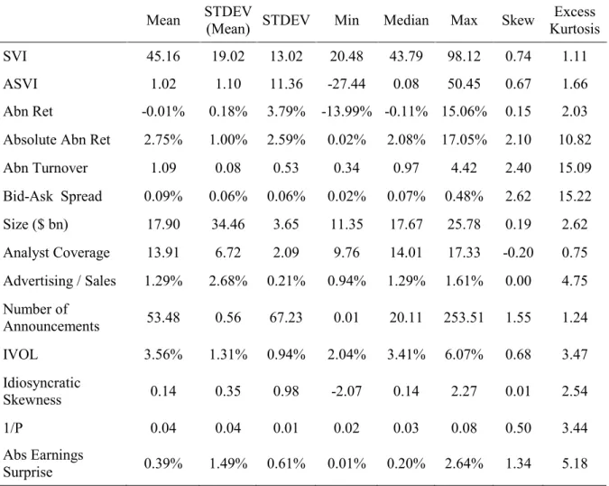
Table 2 reports several descriptive statistics. In a first step, they are computed in the time series of each stock with at least 52 weeks of data and then averaged across all stocks. The exception is the statistic ‘STDEV (Mean)’, where the second step is the standard deviation of each variable’s mean across all firms. It evaluates whether the mean statistic of each variable differs considerably across firms.
We can see there is an average search interest of 45, which is in line with the claim in section 4.1 that these are widely followed companies. In addition, the ‘STDEV (Mean)’ of SVI is 19, indicating that people are not equally interested about all companies. Despite the relatively high average interest, we can still find meaningful variations over time, similar in magnitude to Cziraki et al. (2017). The standard deviation of ASVI is 11.4, which tells us there should be enough dispersion for SVI to work well with large stocks.
As in Drake et al. (2012), it is clear we are in the presence of large stocks. Analyst coverage is on average high, with around 14 analysts following each company, but the attention environment is once again not equal for every firm. The average market cap is $17.9bn, but there are large differences across firms due to outliers such as Exxon Mobil with $500bn in mid-2004. The lack of sample variation in the bid-ask spread, where half of the sample has
Table 2. Summary Statistics
This table shows descriptive statistics for all non-dummy variables defined in table 1 but without any log transformation. They are first calculated for each firm with at least 52 weeks of data and then averaged across all firms. ‘STDEV (Mean)’ stands for the standard deviation of each variable’s mean statistic across all firms. ‘STDEV’ stands for the average of each variable’s standard deviation across all firms. The sample includes 728 companies with weekly data from January 2004 to April 2008, but the data is unbalanced.
Mean STDEV (Mean) STDEV Min Median Max Skew Excess Kurtosis
SVI 45.16 19.02 13.02 20.48 43.79 98.12 0.74 1.11
ASVI 1.02 1.10 11.36 -27.44 0.08 50.45 0.67 1.66
Abn Ret -0.01% 0.18% 3.79% -13.99% -0.11% 15.06% 0.15 2.03 Absolute Abn Ret 2.75% 1.00% 2.59% 0.02% 2.08% 17.05% 2.10 10.82
Abn Turnover 1.09 0.08 0.53 0.34 0.97 4.42 2.40 15.09 Bid-Ask Spread 0.09% 0.06% 0.06% 0.02% 0.07% 0.48% 2.62 15.22 Size ($ bn) 17.90 34.46 3.65 11.35 17.67 25.78 0.19 2.62 Analyst Coverage 13.91 6.72 2.09 9.76 14.01 17.33 -0.20 0.75 Advertising / Sales 1.29% 2.68% 0.21% 0.94% 1.29% 1.61% 0.00 4.75 Number of Announcements 53.48 0.56 67.23 0.01 20.11 253.51 1.55 1.24 IVOL 3.56% 1.31% 0.94% 2.04% 3.41% 6.07% 0.68 3.47 Idiosyncratic Skewness 0.14 0.35 0.98 -2.07 0.14 2.27 0.01 2.54 1/P 0.04 0.04 0.01 0.02 0.03 0.08 0.50 3.44 Abs Earnings Surprise 0.39% 1.49% 0.61% 0.01% 0.20% 2.64% 1.34 5.18
weekly spreads lower than 0.07%, may cause this variable to be insignificant. We can also see the effect of the earnings season, with an average of 53 companies reporting their quarterly results on the same week. Many variables have high enough average skewness and excess kurtosis to make a log transformation useful. In the case of idiosyncratic skewness and abnormal returns, this is not applied because these sample statistics would actually increase. Following Da et al. (2011), when a variable can take the value of zero, such as the bid-ask spread, I sum one before apply the log.
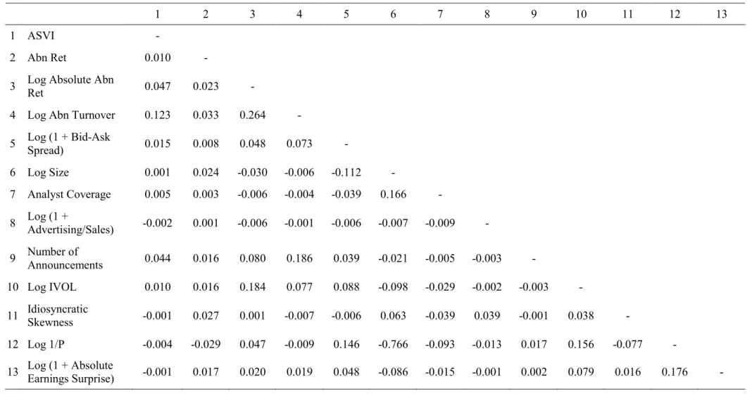
Table 3 presents a correlation matrix following the method of table 2 and Da et al. (2011). Overall, the results are aligned with expectations. There is practically no correlation between ASVI and the other variables, meaning that Google search is capturing an unrelated event. The
Table 3. Correlation Matrix
This table presents contemporaneous correlations for all non-dummy variables defined in table 1. They are first calculated for each firm with at least 52 weeks of data and then averaged across all firms. The sample includes 728 companies with weekly data from January 2004 to April 2008, but the data is unbalanced.
1 2 3 4 5 6 7 8 9 10 11 12 13
1 ASVI -
2 Abn Ret 0.010 -
3 Log Absolute Abn Ret 0.047 0.023 -
4 Log Abn Turnover 0.123 0.033 0.264 -
5 Log (1 + Bid-Ask Spread) 0.015 0.008 0.048 0.073 -
6 Log Size 0.001 0.024 -0.030 -0.006 -0.112 - 7 Analyst Coverage 0.005 0.003 -0.006 -0.004 -0.039 0.166 - 8 Log (1 + Advertising/Sales) -0.002 0.001 -0.006 -0.001 -0.006 -0.007 -0.009 - 9 Number of Announcements 0.044 0.016 0.080 0.186 0.039 -0.021 -0.005 -0.003 - 10 Log IVOL 0.010 0.016 0.184 0.077 0.088 -0.098 -0.029 -0.002 -0.003 - 11 Idiosyncratic Skewness -0.001 0.027 0.001 -0.007 -0.006 0.063 -0.039 0.039 -0.001 0.038 - 12 Log 1/P -0.004 -0.029 0.047 -0.009 0.146 -0.766 -0.093 -0.013 0.017 0.156 -0.077 -
exceptions are absolute abnormal returns and abnormal turnover, where the correlations are 4.7% and 12.3%, respectively. If ASVI is to capture investor attention, it should be positively correlated with returns and trading volume (e.g., Preis et al., 2010; Vlastakis and Markellos 2012). However, the correlations are still relatively low, which is in light with the argument of Da et al. (2011) that returns and turnover are the outcome of several economic factors (e.g., changes in company growth prospects). Interestingly, there is a significant positive correlation of 26.4% between absolute abnormal returns and abnormal turnover, which is not far from the 31.1% reported by Da et al. (2011).
Furthermore, there is a negative correlation of -11.2% between size and the bid-ask spread, which is in line with the idea that smaller stocks are more illiquid (e.g., Amihud, 2002). Given the lack of small stocks in this sample, this is good news about the usefulness of the bid-ask spread as a liquidity proxy. We can also see that smaller stocks have higher idiosyncratic volatility, similar to what Kumar (2009) finds. In addition, size has a correlation of 16.6% with analyst coverage, which is intuitive because it is well documented that larger firms have more analyst forecasts (e.g., Chordia et al., 2007). As a last remark, given that size is the product of shares outstanding with price, its high negative correlation with 1/P is expected.
4.5 Univariate tests
The first univariate test considered here is the cross-sectional dependence (CD) test of Pesaran (2015). Its null hypothesis is that a variable has weak CD whereas the alternative is strong CD. The results are shown in table 4 and the null hypothesis is always rejected. Obviously, given the large sample, with approx. 150,000 observations, it is easy to reject the null even with a very small magnitude (Baltagi, 2009). Nevertheless, several variables report average cross-sectional correlations above 9%, indicating it might be prudent to control for cross-sectional dependence in the regressions. In section 5, this test is also applied to the residuals of each regression given the arguments of Thompson (2010) discussed in section 3.2. Note that the variable number of announcements has a nearly perfect cross-correlation of 99% because, by definition, the total number of earnings announcements at a given week is the same for all firms. Therefore, I expect that this variable cannot be statistically significant with the CCEMG estimator.
The second univariate test is non-stationarity. In the context of hypothesis 3, it implies that: the time-series average of the cross-sectional coefficients as in Fama and
MacBeth (1973) may not converge to the population estimates (Chordia et al., 2007 p. 718).
Table 4. Univariate Tests
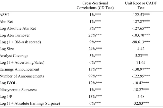
This table shows the results of two univariate tests using all variables defined in table 1 (except for consumer industry). The test on cross-sectional dependence (CD) is the one of Pesaran (2015), where the null hypothesis is weak CD. The numbers represent the average cross-sectional correlations of each variable. Testing for unit roots is done with the CADF test of Pesaran (2007), where the null hypothesis is non-stationarity for all firms. This test is conducted with an intercept and two lags but also a linear time trend for four variables: log size, analyst coverage, log of one plus advertising over sales, and log 1/P. The numbers on the third column represent t-statistics of the CADF test, whose critical values at the 1% significance level are -3.84 (no trend) and -4.31 (with trend). The sample includes 739 companies with unbalanced weekly data from January 2004 to April 2008. *, **, *** represent statistical significance at the 10%, 5%, and 1% level, respectively.
Cross-Sectional
Correlations (CD Test) Unit Root or CADF Test
ASVI 1%*** -122.53***
Abn Ret 1%*** -127.87***
Log Absolute Abn Ret 3%*** -127.65***
Log Abn Turnover 25%*** -103.70***
Log (1 + Bid-Ask spread) 9%*** -98.613***
Log Size 24%*** 4.42 Analyst Coverage 3%*** -5.23*** Log (1 + Advertising/Sales) 0%*** 71.65 Earnings Announcement 13%*** -130.97*** Number of Announcements 99%*** -122.95*** Log IVOL 12%*** -10.42*** Idiosyncratic Skewness 1%*** -18.27*** Log 1/P 13%*** 5.48
Log (1 + Absolute Earnings Surprise) 0%*** -32.83***
More generally, it gives rise to a spurious relation between variables, leading to unreliable inference (Granger and Newbold, 1974). Under large N and T, Phillips and Moon (1999) show there is no problem as long as weak CD holds, which is not the case here. Therefore, I use the cross-sectionally augmented Dickey-Fuller (CADF) test of Pesaran (2007), which allows strong CD. The null hypothesis is that a given variable is non-stationary for all firms while the alternative is stationarity for at least one firm. Following Chordia et al. (2007), the potential candidates are 1/P, size, and analyst coverage, but also advertising over sales due to its much lower (annual) frequency.
In table 4, as suspected, the null of non-stationarity is not rejected for size, advertising over sales and 1/P. To make them stationary, I follow Chordia et al. (2007) and take the residual after regressing each variable on a linear and quadratic time trends as well as 51 week dummies.