1
Equity Valuation – Aena, SA
Maria Inês Viegas Aleixo de Matos | 152114124 Supervisor: José Carlos Tudela Martins
MSc in Management
Dissertation submitted in partial fulfilment of requirements for the degree MSc in Management at the Universidade Católica Portuguesa, 30th December 2015
2 Abstract
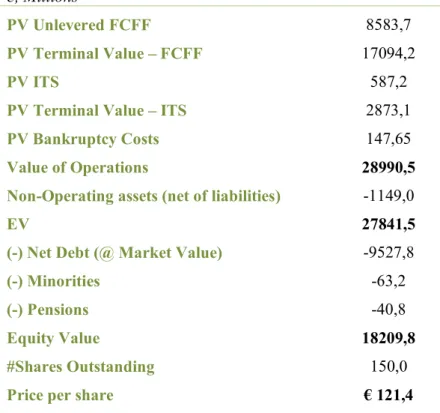
This dissertation presents the valuation of Aena SA, traded on Madrid Stock Exchange. Two methods were applied – Adjusted Present Value and Relative Valuation – and a sensitivity analysis was performed to challenge the values obtained. Through Adjusted Present Value methodology a share price of €121,4 per share was obtained. Thus, an Overweight recommendation applies. Relative valuation was considered only as a validation tool and, therefore, the recommendation was not based on its results. Lastly, a comparison was made between the results obtained on the dissertation and the ones reported by J.P. Morgan Cazenove investment bank on 25 June 2015, highlighting the major differences between the two.
3 Resumo
Esta dissertação apresenta a avaliação da Aena SA, listada na bolsa de Madrid. Dois métodos foram usados – Valor Presente Ajustado e Avaliação Relativa – e uma análise de sensibilidade foi elaborada para desafiar os resultados obtidos. Através do método do Valor Presente Ajustado, um preço por ação de €121,4 foi obtido. Assim sendo, uma recomendação de compra aplica-se. A Avaliação Relativa foi apenas considerada como ferramenta de validação e, assim sendo, a recomendação não foi baseada nos resultados nesta obtidos. Por último, uma comparação foi feita entre os resultados alcançados na dissertação e aqueles apresentados pelo banco de investimento J.P. Morgan Cazenove a 25 de Junho de 2015, destacando as diferenças entre as duas avaliações.
4 Acknowledgments
Firstly, I want to thank to Professor José Carlos Tudela for his availability and valuable insights during these last months.
Secondly, I must thank to my family and to Eduardo for all they support and availability in the most challenging moments. I also want to thank to António for the all the discussions and valuable insights.
Additionally, I would like to say thank you to all my friends, especially Rita, Joana and Bárbara for all their help.
6 List of Abbreviations
ACI Airports Council International
APV Adjusted Present Value
CAGR Compounded Annual Growth Rate
CAPEX Capital Expenditures
D&A Depreciations and Amortizations
DCF Discounted Cash Flow
EBIT Earnings Before Interest and Taxes
EBITDA Earnings Before Interest, Taxes, Depreciations and Amortizations
EV Enterprise Value
FCFE Free Cash Flow to Equity
FCFF Free Cash Flow to Firm
GDP Gross Domestic Product
IATA International Air Transport Association
ITS Interest Tax Shields
NWC Net Working Capital
PVITS Present Value Interest Tax Shields
ROIC Return On Invested Capital
t Tax Rate
7
Index
1. Introduction ... 11
2. Literature Review ... 13
2.1. Discounted Cash Flow valuation methods ... 13
2.1.1. Cash Flows ... 13 2.1.2. Time frame ... 14 2.1.3. Discount Rates ... 16 2.2. Relative Valuation ... 23 2.2.1. Peer Group ... 24 2.3. Aena’s case ... 24 3. Industry Overview ... 25
3.1. Airports trends and characteristics ... 25
3.2. Deal activity ... 27 3.3. Industry Drivers... 27 3.3.1. Air traffic ... 27 3.3.2. Tariffs ... 29 3. Aena S.A. ... 31 3.3. Shareholder structure... 31 3.4. Share Price... 32 3.5. Traffic ... 32 3.6. Tariffs ... 33 3.7. Historical Performance ... 34 3.7.2. Revenues ... 34 3.7.3. Operating expenses ... 36
3.7.4. Capital Expenditures and Depreciations & Amortizations ... 37
3.7.5. Net Debt ... 38
3.7.6. Working Capital ... 39
3.8. Risk Parameters ... 40
4. Company Valuation ... 43
4.3. Explicit period and Terminal Growth Rate ... 43
4.4. Operational forecasts ... 44
8
4.4.3. Operating Expenses ... 48
4.4.4. Operational results ... 49
4.4.5. Capital Expenditures and Depreciations & Amortizations ... 50
4.4.6. Working Capital ... 51
4.4.7. Dividends ... 52
4.5. APV Valuation ... 53
4.5.2. Discount Rate ... 53
4.5.3. FCFF ... 54
4.5.4. Debt Plan and Interest Tax Shields ... 55
4.5.5. Bankruptcy costs ... 56
4.5.6. Results ... 57
4.5.7. Sensitivity Analysis ... 58
4.6. Multiples valuation ... 59
4.7. Recommendation ... 61
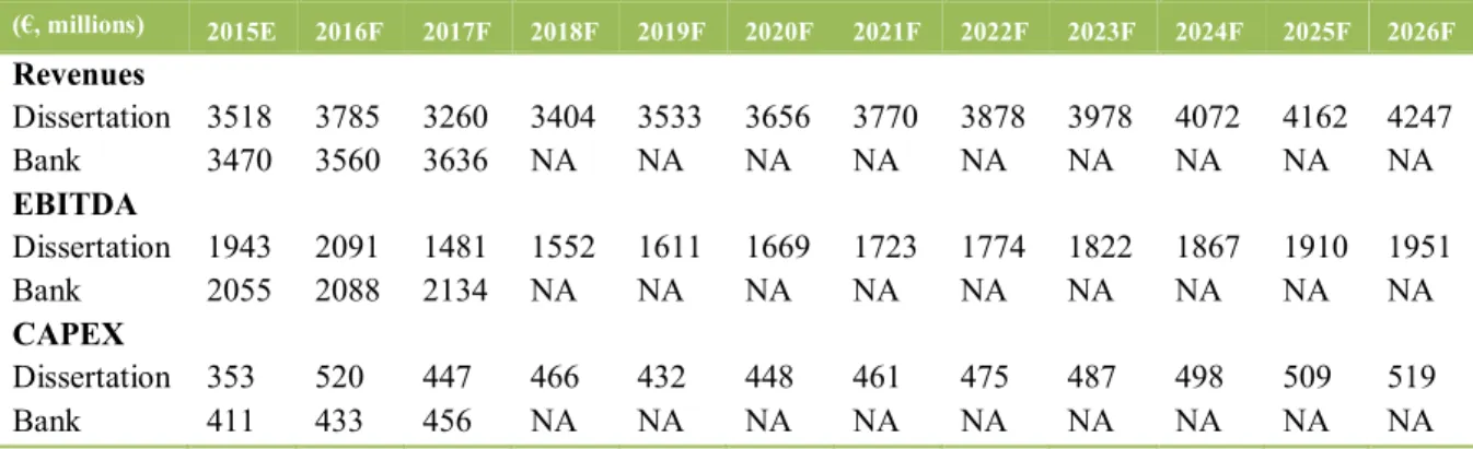
5. Equity Research Comparison ... 63
6. Conclusion ... 65
7. Appendixes ... 67
9
Graph 1: Airport Industry Dynamics ... 25
Graph 2: Global air traffic evolution ... 28
Graph 3: Aena’s Ownership ... 31
Graph 4: Aena’s Stock Price evolution vs IBEX 35 ... 32
Graph 5: Aena’s traffic evolution 2000-2015 ... 33
Graph 6: Regulation Schedule ... 34
Graph 7: Total revenue 2011-2015 ... 34
Graph 8: Distribution of total revenue per segment: A-2013 B-2014 ... 35
Graph 9: Operating Expenses 2011-2015 ... 36
Graph 10: Operating Expenses Composition (2011-2015) ... 37
Graph 11: CAPEX and D&A 2011-2015 ... 38
Graph 12: Net Debt 2011-2015 ... 39
Graph 13: Working Capital 2011-2015 ... 40
Graph 14: Aviation revenue 2012-2026 – Drivers ... 45
Graph 15: Commercial revenue 2012-2026 – Drivers ... 46
Graph 16: Off-terminal services revenue 2012-2026 – Drivers ... 47
Graph 17: International revenue 2016-2026 – Drivers ... 48
Graph 18: Operating Expenses forecast 2012 -2026 – Drivers ... 49
Graph 19: CAPEX and D&A forecast 2016-2021 ... 51
10
Table 1: Percentage of non-aeronautical profits subsidizing aeronautical segments 2014-2018 ... 33
Table 2: Operating Expenses as percentage of revenues (2011-2015) ... 36
Table 3: Spain and World GDP's growth rates forecast 2016-2026 ... 44
Table 4: Passengers' Evolution: Spanish and International 2016-2026 ... 44
Table 5: Maximum allowed revenue per passenger 2015-2026 ... 45
Table 6: EBITDA margin forecast 2016-2021 ... 49
Table 7: EBITDA margin of closest peers forecast ... 50
Table 8: Net Working Capital changes forecast 2016-2026 ... 52
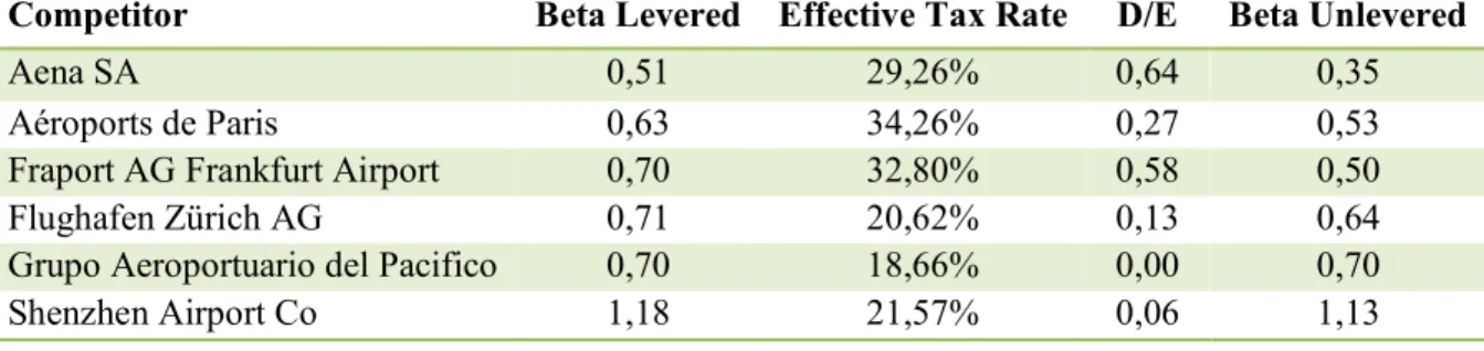
Table 9: Unlevered Beta Calculation ... 54
Table 10: Unlevered cost of equity calculation ... 54
Table 11: FCFF 2016-2026 and Terminal Value ... 55
Table 12: Debt level and interest expenses schedule 2016-2026 ... 56
Table 13: ITS 2016-2026 and Terminal Value ... 56
Table 14: APV Valuation ... 57
Table 15: Tariff level scenarios ... 58
Table 16: Sensitivity Analysis ... 58
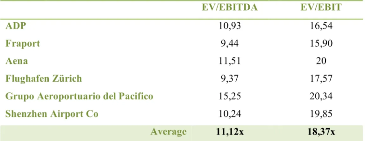
Table 17: Peer group EV/EBITDA and EV/EBIT ... 59
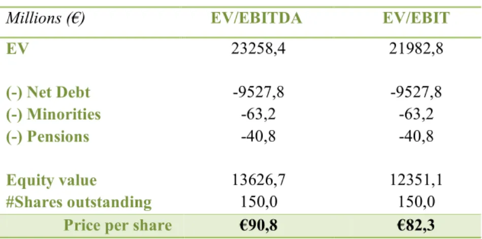
Table 18: Extended peer group multiples’ valuation ... 60
Table 19: Restricted peer group multiples' valuation ... 60
11
1. Introduction
During the last years, the world’s economy has been facing several challenges, following the financial crisis, which led to changes in the way investors act and companies behave.
These years have been characterized by changes in several sectors with mergers & acquisitions and privatizations in some sectors as telecommunications, transportation and infrastructures’ management.
Therefore, Aena appears as a challenging company to value at the moment. An airport operator, which performance seems to be linked to economic recovery, operating in Spain and internationally and that went through an IPO process recently.
This dissertation is organized as follows: firstly, a chapter with state of art, the description of valuation models already developed and different perspectives; secondly, an overview of the airports’ management industry; thirdly, a company overview, where Aena’s reality and past financial performance is presented; fourthly, the company’s valuation, based on our assumptions on main financial drivers, followed by a sensitivity analysis; lastly, a comparison between the dissertation valuation’s result and the one of an investment bank is made, explaining the main differences between them.
13
2. Literature Review
In this section, we will describe the main methods used in equity valuation exercises, namely the Discounted Cash Flow methodologies and the Relative Valuation technique.
2.1. Discounted Cash Flow valuation methods
Several authors agree to consider Discounted Cash Flow (DCF) method as the most accurate when valuing a company or on the decision process to pursue, or not, a specific project. DCF is based on the principle of valuation, which states that the “value of any asset is the present value of expected future cash flows that the asset generates” (Damodaran, 2002). Moreover, the value of an asset today results from the discount of the expected future cash flows at an appropriate rate.
In the following chapters, we will present the following cash flow methods: Weighted Average Cost of Capital (WACC), Adjusted Present Value (APV) and Dividend Discount Model (DDM).
2.1.1. Cash Flows
Kaviani (2013) presents two possible ways to use cash flows when doing a DCF valuation: one can decide to use Free Cash Flow to Firm (FCFF) or Free Cash Flow to Equity (FCFE). FCFF represents the cash flow available for both equity and debt holders, while FCFE reflects only the cash available to equity holders, after the commitments to other stakeholders paid (Mitra, 2010).
FCFF is calculated according to the following formula:
According to Koller et al (2010), to obtain the Enterprise Value (EV), one should discount FCFF at a rate that takes into account the remuneration for both equity and debt holders, the Weighted Average Cost of Capital (WACC), a term that will be discussed further on. Thus, firm value can be computed as:
14 Regarding FCFE, it can be computed as follows:
The value of the equity of a firm can be computed by discounting FCFE at an appropriate rate. However, as stated in Mitra (2010), since FCFE considers only the cash flows available to firm’s shareholders, the appropriate discount rate is no longer WACC, but the cost of equity, 𝑟𝑒, the shareholder’s required rate of return. Therefore, the equity value is given by:
Theoretically, if assumptions are consistent and representative of the surrounding environment, one should obtain the same equity value independently of the approach chosen. Nevertheless, there are some situations where FCFF approach is preferable: if the firm’s FCFE is negative and/or the capital structure is unstable1.
2.1.2. Time frame
Equations 2 and 4 present the value of the firm and the value of its equity, respectively, as an infinite sum of discounted cash flows (FCFF and FCFE). Although this computation may seem intuitive, it is not feasible, since one cannot estimate these cash flows indefinitely. In order to overcome this limitation, DCF valuation is presented in Young et al. (1999) as a sum of two parts: the explicit period forecasts and the terminal value.
2.1.2.1. Explicit Period
The question arising at this stage is how long should the explicit period be and which criteria should be fulfilled in order to consider that, from that year onwards, the cash flows will “grow at a constant perpetual growth rate”2.
1 Cost of equity becomes highly volatile when capital structure is not stable.
2 Cassia, Lucio, Andrea Plati, and Silvio Vismara. "Equity valuation using DCF: A theoretical analysis of the long term hypotheses." Investment Management & Financial Innovations 4.1 (2007): 91-108.
15 Copeland et al. (2000) argue that the time frame of the explicit cash flow forecast should be, at least, as long as the time that the company takes to achieve its steady state. Cassia et al. (2007) add that, when the steady state is reached, the company has already exhausted its sources of competitive advantage.
Several authors consider as a reasonable time frame five to ten years of explicit forecast period, depending on the specific characteristics of the company as its “size, growth rate and excess returns, and scale and sustainability of competitive advantages” (Damodaran, 2002).
Empirical studies, as the ones presented by Penman and Sougiannis (1997) and Sougiannis and Yaekura (1997), show that, as the explicit period becomes longer, the presence of valuation errors decrease in a monotonous way. Nevertheless, Ohlson and Zhang (1999) state that precaution is still needed.
2.1.2.2. Terminal Value
As stated above, the second moment of the valuation is related with the computation of the terminal value.
The majority of the analysts do not give the attention needed to this calculation. Young et al. (1999) highlight the danger related with these practices, since “80% to 90% of analysts’ time is spent calculating a parcel that corresponds to only 10% to 20% of the final market value estimate”.
Damodaran (2002) presents three ways to find the terminal value: liquidation value, multiples, and stable growth model.
The first one assumes the company will cease its operations in the terminal year and sell its assets. The estimation of the assets’ value is called liquidation value.
In the second method, the analysts compute the terminal value using multiples. Even though this method stands out for its simplicity, it could lead to a dangerous combination of relative and DCF valuation. One should bear in mind that an estimate of the intrinsic value should be the result of a DCF valuation, and not one of a relative value.
Lastly, the stable growth model assumes that the firm will grow at a constant rate (𝑔𝑠𝑡𝑎𝑏𝑙𝑒)
16
In this computation, the cash flow and discount rate will depend on the type of valuation being made: when valuing equity, the cash flow is the cash flow to equity and the discount rate is the cost of equity; when computing firm’s value, the cash flow is the cash flow to firm and the discount rate the cost of capital.
The stable growth rate assumes a key role in the final estimate, since a minimal change in its value will lead to a significant change in the terminal value, whose main importance was already discussed above.
The value to attribute to the stable growth rate is, therefore, a main concern. Although there is not an explicit rule to define the stable growth rate level, this rate cannot be higher than the growth rate in the domestic economy (if the company operates only domestically), or higher than the global economy’s growth rate (if the company is a multinational or intends to be). Simultaneously, some authors argue that a good assumption to make is that the company, especially if mature, will grow at a rate lower than this imposed limit.
2.1.3. Discount Rates
A common characteristic of all discount cash flow methodologies is the presence of a discount rate. In every situation, this discount rate should represent, adequately, the reality faced by the investors, namely in what concerns risk faced (Koller et al., 2010).
The discount rate used should be aligned with the specificities of the company of interest and with the cash flows being discounted.
2.1.3.1. WACC
The most common approach to company valuation is the WACC method. This method computes the firm’s overall cost of capital. Each capital category is weighted, proportionally, as follows:
The cost of debt (𝑟𝑑) and the cost of equity (𝑟𝑒) are both opportunity costs, each resulting from
17 are done with after-tax cash flows, interests paid to debt holders are tax exempt, being the cost of debt reduced to account for these benefits, [𝑟𝑑× (1 − 𝑡)].
When computing WACC some attention is required. Firstly, one should consider the market values of debt and equity, and not their book values. Secondly, as Fernandez (2004) highlights, one should consider the effective tax rate faced by the leveraged company, instead of the statutory tax rate.
Luehrman (1997) and Mitra (2010) agree to consider as main advantage of WACC its simplicity as all financing considerations are included in a single discount rate and, therefore, the decision-making process is simplified. Nevertheless, the same authors argue that WACC works properly only for the simplest firms, with static capital structures. The discount rate will change on a year-to-year basis as debt to equity ratio changes. Changes will also occur when the tax structure changes.
Moreover, Luehrman (1997) states that there is a high probability of interest tax shields being misvalued when using WACC as the discount rate.
In the next chapters, we will attempt to describe both the cost of equity and cost of debt.
Cost of equity
Several models have been developed to estimate the cost of equity, being the most widely use the Capital Asset Pricing Model (CAPM), the Fama-French Factor Model and the Arbitrage Price Theory (APT).
Sharpe (1964), Lintner (1965), Mossin (1966) and Treynor (1965) developed independently the CAPM. This one-period model considers that investors are compensated in two ways: time value of money, represented by the risk-free rate, and risk.
Risk is divided into two categories: the systematic risk, 𝛽, which cannot be diversified and results from the “exposure to the economic activity”; and the unsystematic risk, which can be diversified and is related with “stock specific risks” (Sharpe, 1964). Thus, the investors are only compensated for the specific risk “proportionally to their risk exposure”. Cost of equity is therefore computed as follows:
18 CAPM has some underlying assumptions. The model considers that all investors are price-takers and that they care about “returns measured over one period (static view)”. Moreover, it also assumes that there are no non-traded assets, no taxes nor transaction costs.
Fama and French (1993,1996) argue that CAPM presents several empirical failings, mainly due to its simplifying assumptions. While CAPM considers that the degree at which a security moves with the market is the main factor influencing its price, Fama and French add size and value factors to the equation.
Developed by Ross (1976), APT states that two portfolios with the same level of exposure to risk have to earn the same return. The rate of return depends on the exposure to both market and firm specific risks.
One can therefore conclude that the cost of equity is open to a fair amount of controversy. Thus, analysts working with cost of equity seek to use models that are commonly used to reduce this mystic around its computation. Therefore, we will compute cost of equity using CAPM.
i) Risk free
Damodaran (2008) considers an asset as risk free if its actual return matches exactly the value of its expected return. In order to fulfill this requirement, two conditions must be verified: there are “no default and reinvestment risks associated with the asset”.
Considering these criteria, Koller et al. (2010) conclude that the only risk-free assets are the long-term government bonds, given that those entities have the ability to issue money, when needed3.
To be more accurate, one should discount each cash flow with the correspondent government bond, in terms of maturity (Koller et al., 2010). Nevertheless, the majority of analysts prefer to work with a “single yield to maturity that represents the entire cash flow stream being valued”4.
Typically, finance professionals use US treasury bonds with 10 years maturity5 as risk free
when valuing a US based company and the German bunds, with same maturity, when valuing
3 When compared with the Federal Reserve, the European Central Bank presents a more limited monetary policy. 4 Koller, T., Goedhart, M., & Wessels, D. (2010). Valuation: measuring and managing the value of
companies (Vol. 499). john Wiley and sons: 241
5 Longer maturities as 30 years might be a better proxy to the cash flow stream. However, due to illiquidity the price and yield premium may not be a good proxy to current value.
19 European companies.
Moreover, one should take into account that the government bond rate should be in the same currency as the cash flows of interest (Koller et al., 2010).
ii) Beta
To compute the expected return of a stock, through CAPM, one needs to compute the stock’s beta. Beta measures the systematic, or non-diversiable, risk of a stock vis-à-vis the market as a whole.
Ross (1976) defines beta as “the covariance between the return on the asset and the market portfolio”, normalized by the variance of the market portfolio.
Depending on the capital structure of the company of interest, levered or unlevered, the analysts should use one of the following equations:
The first equation should be used when WACC applies, while the second one should be used in APV, where the firm is considered all equity financed.
Damodaran (2002) states that if one assumes debt carries no market risk, levered and unlevered betas relate as follows:
According to Damodaran (2002), there three alternatives to compute beta.
Firstly, the historical market betas’ procedure. In this case, beta results from the “regression of the historical returns on the investment against the historical returns on a market index”. Even though it is a widely used approach for publicly traded firms, the author highlights some constraints as the choice of the market index, the length of the estimation period and the choice of a return interval.
20 firm’s beta is computed based on a set of comparable, publicly traded, companies.
Lastly, the third approach considers accounting parameters to estimate the market risk. Nevertheless, this method presents major problems as the potential manipulation of accounting earnings and their exposure to non-operating items.
Blume (1971) shows that, over time, betas tend to present “mean reverting properties”, meaning they revert towards 1. Therefore, in order to forecast future betas with lower estimation errors, analysts may use the following formula:
iii) Market risk premium
Market risk premium is a relevant parcel when computing the cost of equity and one of the most debated topics in finance.
Fernandez (2004) defines it as the “incremental return of a diversified portfolio (the market) over the risk free required by an investor”. The author highlights that CAPM assumes that the risk free is given by long-term treasury bonds’ yields. Moreover, this required premium would be as higher as the investor perceived risk.
The mostly used method to estimate market risk premium uses historical returns, being the expected risk premium the difference between annual returns on stocks versus bonds over a long time horizon (Damodaran, 2015). Nevertheless, critics have emerged with empirical studies, as Fernandez (2004), considering the method provides inconsistent results overstating the required market premium.
Damodaran (2015) presents two more approaches to compute market risk premium. The first one is based on surveys to investors and managers in order to understand which are they expectations regarding equity returns in the future. The second one is the implied approach, where, instead of a backward looking as in the historical returns’ method, a forward-looking estimate of the market premium is computed using either current equity prices or risk premiums in non-equity markets.
21
Cost of debt
In the previous section, we have analysed the cost of equity and the required values to use in its computation. However, the majority of businesses finance their operations using other finance instruments apart from equity, as debt and some hybrid6 securities.
The costs faced by lenders are considerably different from the ones faced by equity holders and, therefore, one should take them into account, proportionally to its stake in the company, when computing the cost of capital.
Lenders could incur in a loss if the firm fail to pay its commitments, namely the interest expenses and principal repayment.
The cost of debt (𝑟𝑑) considers, mainly, three variables: the risk-free rate, the default risk and
the tax advantage associated with debt. Firstly, the higher the risk-free (𝑟𝑓), the higher the cost
of debt the company will face. The same is true when considering the default perceived risk, which will increase the default spread and, therefore, the cost of debt. Lastly, equity and debt present different tax treatments - equity cash flows are paid with after-tax cash flows, while interest payments are tax deductible.
2.1.3.2. APV
As previously discussed, WACC could lead to some errors due to its simplicity.
Myers (1974) presents a better approach to value a business operation, the Adjusted Present Value (APV) method. The author considers two categories of cash flows: cash flows associated with the business operation (revenues, cash operating costs, and capital expenditures); and “side effects”, related with the firm’s financing program (interest tax shields, subsidized financing, issue costs, and hedges).
Moreover, the cash flows coming directly from the business operations are “adjusted for” the side effects on other investments and financing options, as follows:
Firstly, the firm is valued as if it was only equity financed. Therefore, the unlevered cash flows
22 are discounted at the unlevered cost of equity (equation 9). Secondly, the financing side effects – Interest Tax Shields (ITS), costs of financial distress, subsidies, hedges, issue costs, among other - are added.
ITS are computed by multiplying the interest level by the tax rate faced by the corporation. Afterwards, their present value is computed by discounting them at 𝑟𝑢 or 𝑟𝐷, depending if debt
is expected to follow company’s assets behaviour or not.
APV method appears as a better option when the company intends to change its debt-to-equity ratio. Further, Luehrman (1997) considers APV as a better tool since it helps managers to access, not only the value of an asset, but also from where that value comes from. Nevertheless, APV and WACC, if applied correctly, in the majority of the situations, should yield identical results.
2.1.3.3. Dividend Discount Model
Literature considers Dividend Discount Model (DDM) as the simplest method to value equity (Damodaran, 2006).
In this case, the current price of a stock is given by the present value of its future dividends, trough infinity, discounted at the cost of equity. Therefore, the price of the stock today is computed as:
Nonetheless, in reality, one cannot make assumptions about expected dividends to infinity. Thus, some models have emerged to overcome this situation.
An example is the Gordon Growth Model, by Gordon and Shapiro (1956), which considers that the firm is in steady state with dividends growing at a perpetual stable rate. This model provides more accurate results to firms that present a growth rate similar or lower than the nominal growth rate of the economy and whose dividend payout policies are well established and intend to continue into the future (Damodaran, 2006).
Even though DDM is considered the simplest method to value equity, it is important to bear in mind that it presents several limitations, being the more relevant the easy manipulation of dividends. To distribute dividends is a purely strategic decision and does not translate the company’s health.
23
2.2. Relative Valuation
An alternative to the discount cash flow valuation techniques, previously presented, is the valuation using multiples.
Lie and Lie (2002) describe this method as a two-step process. Firstly, one should calculate the multiples for a set of similar companies and, afterwards, use those to find the implied value of the company of interest.
In fact, more than an alternative to other valuation methods, several authors consider valuation using multiples a complement to these other techniques. Fernandez (2015) states that multiples should be used in a second phase of the valuation process, after performing the valuation using another method. Following the same rational, Goedhart et al. (2005) consider that an accurate analysis comparing a company’s multiples with those of other similar firms could be of the major importance to test the validity of the cash flow forecasts made previously and to analyse the strategic potential of the company vis-à-vis other industry players.
Valuation using multiples presents a high adoption rate by analysts and managers. Damodaran (2002) presents three main reasons for the attractiveness of this method: multiples valuation requires fewer assumptions than a DCF valuation; managers and, especially clients, find it easier to understand than a DCF valuation; and, it is a more accurate estimate of the market current mood.
Nevertheless, multiples have some drawbacks associated. Damodaran (2002) identifies three of them: multiples can generate inaccurate estimates of value if key variables as risk, growth or cash flow potential are neglected; moreover, the fact that the valuation is based on similar companies can lead to an overvalued company, if the markets are particularly optimistic and, therefore, overvaluing the comparable firms, or to an undervalued company, if the markets are not so confident about the comparable firms; finally, the lack of transparency associated with the underlying assumptions may lead to manipulation.
Regarding the time horizon when computing multiples, the principles of valuation enhanced by the existent literature state that valuations are more accurate if forward-looking multiples are used instead of trailing multiples, as reported in Liu et al. (2002) and Goedhart et al (2005), unless no reliable estimates are available7.
The most used multiples are the Price-Earnings (PER) and the Enterprise Value-EBITDA (EV/EBITDA). Nevertheless, some authors have expressed a preference for the second one,
24 since PER is highly affected by the capital structure and is based on earnings, which can be easily manipulated.
2.2.1. Peer Group
The main question when computing multiples is to find a set of comparable firms. However, the main question is “What is a truly comparable firm?”. This question has been widely discussed in literature. Goedhart et al. (2005) state as peers the companies with similar Return-On-Invested-Capital (ROIC) and expectations of long-term growth.
2.3. Aena’s case
After analysing the existent literature, we are now able to conclude which methods better fit the characteristics of Aena, SA.
Regarding the DCF methodologies, we will apply APV since the firm states on its reports that its capital structure will change and, therefore, the WACC approach would not be the most appropriate.
DDM was also excluded from our analysis since it presents a high exposure to dividends manipulation. Additionally, Aena’s dividend policy is expected to change, which sustains our decision of excluding DDM.
Moreover, after applying DCF, we will conduct a sensitivity analysis to observe the influence of certain variables in the firm’s target price.
Additionally, we will apply a relative valuation technique. The multiples chosen were the EV/EBITDA and EV/EBIT, since they are less exposed to capital structure changes than earnings’ multiples and are the most accurate ones to use in relative valuation as stated by Chullen et al. (2015). This method will help us to validate our previous results.
25
3. Industry Overview
In this section we intend to analyse the airport operation industry’s dynamics. We start by identifying the business model of the industry as well as the most relevant trends. Since the industry is highly dependent on air traffic figures and tariff regulations, we will discuss these two issues with more detail.
3.1. Airports trends and characteristics
According to IBISWorld, businesses that “operate international, national or civil airports” comprise the airport operation industry. Additionally, the industry also includes agents that support airports, like parking operators, cargo terminals, luggage and handling services or even aircraft control and maintenance. Usually, a single fixed-base operator provides these services, although some of the services may be managed and operated by other entities.
An airport may be described as a multi-sided market. This means that the airport operates as a platform that connects passengers, both to airlines and to other non-aviation services. This implies that the airport can benefit from the existence of externalities, since passengers are better off if there are more airlines/non-aviation services and vice-versa.
As it can be seen in the following figure, there are complex payment streams and relations between the different agents that must be considered when analysing the airport industry.
Services Tickets
On-board services
Rent (fixed plus variable) Fee per passenger
(maximum defined)
Passengers
Airlines PLATFORM AIRPORT Other
services
Services
26 Nowadays, airports face multiple challenges that impose a continuous drive for efficiency, service and passenger growth. As highlighted by PwC in its report Airport operators’ quest for efficiency (2015), these challenges comprise: the increased expectations, by both passengers and airlines, in what concerns service’s quality; the regulators’ imposed limits on aeronautical charges; and “the need to fulfil a national, regional, or municipal development role”. Therefore, the capacity of airport operators to focus on operating expenses and investments on the areas that provide them unique features, to both passengers and airlines, is crucial to overcome those challenges.
In order to cover their costs, airports have been diversifying their offer with the development of non-aeronautical activities, such as retail, parking, real estate, among others. ACI in its report An Outlook for Europe’s Airports – Facing the Challenges of the 21st Century (2010) states
that these activities represent close to 50% of airport revenues, reaching, in some cases, 70%. In fact, the non-aviation segment is becoming more relevant since “commercial revenues have been growing faster than aeronautical revenues” (Morrison, 2009).
Air transportation has been changing across the world and Europe is not an exception. The new financial reality obliges airports to operate cost efficiently, since they are becoming more independent of public finances, and, at the same time, to respond better and faster to the needs of a diversified customer base. In fact the EU liberalisation policy for airlines had a visible impact over airports, which can no longer rely on their national flag carrier to determine traffic growth. Instead, airports are now continuously competing with each other to capture new customers: passengers, airlines and transporters while airlines pressure airport operators to improve quality services and to decrease costs (Ivaldi et al., 2011).
Another trend has been observed: the emergence of Low Cost Carriers (LCCs). According to the EPRS8 (2014), the European market is the most active one for LCCs business, registering
250 million passenger trips per year.
Moreover, the European airports represent not only an important factor for tourism purposes, but also a relevant decision factor to companies establishing new businesses’ location. Therefore, the local economy can be highly influenced by the airports nearby.
Regarding future challenges, ACI (2010) highlights four: capacity, environmental, connectivity and security challenges. Airports need to plan for possible future increases in capacity, to meet
27 demand, at the same time that they respond positively to increasing environmental concerns. Additionally, airports need to ensure passengers can move easily across different locations, ensuring the maintenance of the required security levels.
A further analysis of the industry dynamics is presented in Appendix 1, through a Porter Five Forces framework.
3.2. Deal activity
Airport privatization and the participation of private operators are now global trends, boosted by the need of governments to look for more efficient ways to manage local airports.
As reported by PwC in Connectivity and growth – Directions of travel for airport investments (November, 2014), the deal activity in the industry has been quite high with a peak of 20 deals in the second half of 2013, amounting to US$13 billion (Appendix 2).
Accordingly to PwC, the drive for privatizations is expected to continue since governments seek to realize cash through asset sales.
3.3. Industry Drivers
An airport operator activity is influenced by a number of factors, just as discussed above. However, there are two main issues that affect extensively its operation: air traffic and tariffs. Thus, we will analyse each of these issues with further detail.
3.3.1. Air traffic
The airport operators’ financial results’ prosperity and the global air traffic numbers are closely intertwined. In fact, one would expect that these two variables are positively correlated. Regarding global air traffic, since 1992 a positive evolution can be observed, with the figures in 2013 being almost three times higher than the ones of 1992 (see graph below). The recent financial crisis has reduced the growth rate of air traffic for some years, although the growth trend was not inverted.
28
Graph 2:Global air traffic evolution (Source: J.P. Morgan)
Global air traffic is expected to maintain its growth trend. Airbus forecasts an annual growth of 4.7%, on average, between 2012 and 2032. IATA and ACI projections confirm this tendency, with a forecasted 4.1% CAGR for the period 2009 to 2029 and 2010 to 2029, respectively.
Given the main relevance of air traffic, and its upward trend, it is important to analyse its drivers in order to understand its impact on airport operators’ financials.
Firstly, the number of air travel passengers has shown, historically, a high correlation with global GDP growth. Data show that the number of passengers increases with economic growth. In fact, IATA (2008) estimates that air traffic increases at a 1,4 proportion with income changes. Moreover, Airbus has also concluded that external industry dynamics, such as financial crisis or even the 9/11 terrorist attacks, do not affect air travel significantly (Appendix 3).
Secondly, as highlighted by EUROCONTROL, the purpose of the journey is also an important factor to consider. The elasticity of air travel demand depends highly on the type of passenger. For instance, leisure passengers react strongly to a shock on their income. If their income is reduced they are likely to reduce significantly their leisure air trips. As leisure trips have a significant expression in the total developed economies’ air traffic, households’ income shocks are likely to affect significantly an airport operator’s finances. Also, it is important to consider that youngest generations might be more comfortable with virtual meetings and, thus, business travels may decrease in the future.
29 There are other factors likely to affect travel patterns such as the possibility of an environmental disaster, terrorism, political instability, human rights violations, or just changes in consumers’ trends and tastes.
3.3.2. Tariffs
Additionally to air traffic level, airport operators’ financial results are strongly influenced by the fees they are able to charge. These fees are mainly applied to passenger travelling, aircraft landing and security measures for the use of the airport service facilities. The level of tariffs allowed is computed under a regulation framework established by national agencies and governments. The regulation set is in place during a determined regulatory period after which the regulator analyses the company performance and determines if major changes are needed. There are two methods to compute the maximum fee airports are allowed to charge: the Rate-of-Return (RoR) and the Price cap mechanism. These two methods are then subject to the regulatory environment in place (single-till, dual-till or adjusted-till), discussed in further detail below.
Under the Rate-of-Return methodology, the regulator establishes a maximum allowed rate of return for the entire regulated entity’s business. Thereafter, the airport is autonomous in establishing its price policy within its network. However, its return on capital cannot be higher than the established allowed return.
In the case of Price cap mechanism, the regulator allows for an average price increase adjusted by a “X” factor. Regarding the average price increase, it is commonly determined based on an available price index as the consumer price index (CPI). The “X” factor is established according to a set of criteria as the productivity level of the industry, the regulator perception in what concerns firm’s cost level, or the performance of the company in the previous regulated period.
Regardless of the method chosen, the regulator considers the future operating CAPEX plans and its efficient utilization in the previous regulatory period when establishing the maximum allowed fee.
Nowadays, different regulatory environments coexist in the European airport operators’ industry: single, dual or adjusted tills.
30 Single-till
Under single-till, the aeronautical charges are computed taking into account the revenues from both aeronautical and non-aeronautical activities. Historically, this regulation has been the most widely used in Europe, being now mainly used in the UK.
Usually the aeronautical charges are lower under this framework, since it considers cross-subsidization between non-aeronautical and aeronautical activities.
Advocates of this approach argue that commercial activity’s profits are directly intertwined with the level of people in the airport, which in turn determines the success of the aeronautical activities.
Dual-till
Contrary to what happens under the single-till framework, under dual-till the aeronautical charges are computed based only on the aeronautical activities. Nowadays, this regulation framework is used in major airports such as Amsterdam and Frankfurt.
Dual-till has gained more supporters, since not only avoids cross-subsidization, but also forces airports to be cost efficient, by deriving the airport fees from the associated costs.
Usually, fees charged under dual-till will be, on average, higher. Nevertheless, this does not mean that passengers will face higher prices, since airlines absorb the increase, to avoid a shock in passengers’ demand.
Adjusted -till
The adjusted-till, also referred as hybrid till, is in between single-till and dual-till frameworks. On one hand, it is not a single-till, since it does not consider all non-aeronautical revenues when computing aeronautical charges. On the other hand, it is not a dual-till, given that some of the non-aeronautical activities may still be regulated together with the aeronautical ones.
This regime aims to encourage airports to operate efficiently and link CAPEX spending with profitability both in aeronautical and non-aeronautical businesses.
Usually, it is used as a transition vehicle from a single-till to a dual-till, or vice-versa. In fact, as Aena is converging towards a dual-till system, currently a hybrid framework is on place.
31
4. Aena S.A.
Aena S.A. is responsible for the management of airports and heliports in Spain. Moreover, through its subsidiary Aena International S.A., it is also present abroad, with participations in the management of 15 international airports. Aena’s operation evolves around four main segments: Aviation, Commercial, Off-terminal services and International (Appendix 4). Regarding its Spanish operation, Aena manages 46 airports and 2 heliports, which have allowed the company to develop expertise and skills to manage airports of different categories and dimensions. The domestic network is organized accordingly to the airports’ annual passenger traffic. There are three main airports – Adolfo Suárez Madrid-Barajas, Barcelona-El Prat and Palma de Mallorca – and the remaining are divided as follows: Group Canarias (given the distance and the importance of inter-islands traffic), Group I (more than 2 million passengers/year), Group II (more than 500 000 passengers/year) and Group III (less than 500 000 passengers/year).
Internationally, Aena is present in three different countries: the United Kingdom (London-Luton Airport, 51% stake), Mexico (Aeropuertos Mexicanos del Pacífico, 33,33% stake) and Colombia (Sociedad Aeroportuaria de la Costa, 37,89% stake; Aerocali, 50% stake).
4.1. Shareholder structure
As the majority of airport operators worldwide, Aena is a state-owned company, being ENAIRE its Parent Company. Nevertheless, and also as verified among other players, Aena is now becoming more independent of public finances, with a free float of 49%.
51% 8% 3% 38% Aena's Ownership ENAIRE
TCI Fund Management Limited
HSBC Holdings PLC Others
32
4.2. Share Price
Aena is listed since 11 February 2015 on Madrid stock exchange. The IPO price was of 58 euros per share, meaning a valuation of 8,7 billion euros.
4.3. Traffic
Aena is the world’s largest airport operator in what concerns passengers’ level. In 2014, traffic reached 206,4 million passengers (both Spanish network and London-Luton airport), a number considerably higher than the ones verified among the main airport operators (Appendix 5). Furthermore, two of Aena’s Spanish network airports – Madrid Barajas and Barcelona El Prat – are among the top ten EU airports in terms of passengers’ level.
Given the company releases, it is possible to analyse the traffic typology in Spanish airports with further detail. Data suggests that there is a relation between the world economic growth and the air traffic level verified. For instance, during the last financial crisis, the international traffic outperformed the domestic one, which could be explained by the strong effects felt on the Spanish economy during this period.
Since 2013, one can observe a positive trend, mainly due to the economic recovery in some tourist-generating countries and to the political and social situation in some alternative destinations. 0 20 40 60 80 100 120
Aena stock price evolution vs IBEX 35 (€)
Aena IBEX 35
33
Graph 5: Aena’s traffic evolution 2000-2015 (Source: Company reports)
A detailed analysis of traffic of the Spanish network and investee airports is presented in Appendix 6. Additionally to the economic recovery, the emergence of LCCs has contributed to the recovery of traffic at Aena, given their relevance among the airlines serving Aena (Appendix 7).
4.4. Tariffs
Aena’s operation is highly regulated. There are limits to the price that can be charged per passenger, among other rules, that are established by the regulator. Regarding the regulatory environment, Aena is now in a transitory phase, denominated hybrid till, towards a dual-till system, which will be reached in 2018. This phase has started in 2014, and, therefore, it has a total duration of 5 years.
From 2014 to 2018, the portion of the non-aeronautical activities’ profits subsidizing the aeronautical business is going to decrease 20% each year. Initially, in 2014, the parcel of non-aeronautical income taken into account will be 80% and, thus, 0% will be reached in 2018.
2014 2015 2016 2017 2018
80% 60% 40% 20% 0%
Table 1: Percentage of non-aeronautical profits subsidizing aeronautical segments 2014-2018 (Source: Company reports)
From 2017 onwards, DGAC (Dirección General de Aviación Civil) will establish the fees to be charged in the following years. These fees are established under DORA (Document of Airport Regulation) agreements, whose length is 5 years. The main objective behind these
34 contracts,which avoid regulatory uncertainty, is to “provide revenue visibility”. On the other hand, Aena has to guarantee that the airport network operations will continue.
Graph 6:Regulation Schedule (Source: Spanish National Authority of Markets and Competition)
4.5. Historical Performance
4.5.1. Revenues
Aena’s total revenues have been increasing, with a CAGR of +6,3% from 2011 to 2014. This positive trend is expected to be maintained in 2015, with total revenues being 11,2% higher than the ones verified in 2014.
Regarding its distribution among the four segments of the company in 2014 – Aviation, Commercial, Off-terminal services and International – aviation accounts for the majority, being
2017
Hybrid-till Dual-till
2013 2021 2026
1st DORA
2nd DORA
Yearly fees increase
2018
CAGR 2011-2014: +6,3%
Graph 7:Total revenue 2011-2015 (€, millions) (Source: Company reports; Own calculations)
35 responsible for 70,82% of total ordinary revenue, followed by commercial activities, 19,89%, off-terminalservices, 5,07%, and international, 1,45%.
All the four segments registered a rise in ordinary revenue in the last years. The international segment had the more significant increase, which is explained by the takeover of London-Luton airport.
However, although revenue in the aviation segment has increased (mainly due to the improvement in traffic), this segment has reduced its influence in Aena’s total revenue from 74,07% in 2013 to 70,82% in 2014. On the other hand, commercial activities (both inside and outside terminals) are increasing their stake in total ordinary revenues; their revenues rise is mainly explained by the new-long term contract signed with World Duty Free Group, the improvement of restaurants and shop areas and the re-launch of parking business. This confirms the industry trend of the increased importance of non-aeronautical activities for the success of airport operators.
Graph 8: Distribution of total revenue per segment: A-2013 B-2014 (%) (Source: Company Reports)
74,07% 18,86%
4,99% 0,28%
Distribution of total revenue per segment 2013 (%)
Aviation Commercial Off-terminal International
70,82% 19,89%
5,07% 1,45%
Distribution of total revenue per segment 2014 (%)
Aviation Commercial Off-terminal International 70,82%
19,89%
5,07% 1,45%
Distribution of total revenue per segment 2014 (%)
Aviation Commercial Off-terminal International
(A)
36
4.5.2. Operating expenses
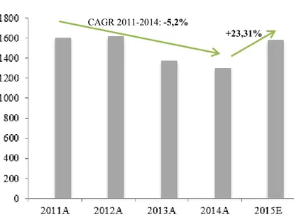
Aena has been implementing since 2012 an efficiency plan, which has contributed to a significant cost reduction. From 2011 to 2014, operating expenses have been reduced at a CAGR of -5,2%.
However, in 2015 an increase is expected, +21,31%, given Luton full consolidation and new security measures.
2011A 2012A 2013A 2014A 2015E
Operating Expenses (% revenues) 64,87% 60,53% 46,80% 41,02% 44,77%
Table 2: Operating Expenses as percentage of revenues (2011-2015) (Source: Own Calculations)
“Other operating expenses” is the largest expense item on Aena’s financials. This item includes several expenses, mainly related to security measures. Staff costs are also significant on Aena’s total expenses.
Graph 9:Operating Expenses 2011-2015 (€ Millions) (Source: Company reports; Own calculations) CAGR 2011-2014: -5,2%
37
Graph 10: Operating Expenses Composition (2011-2015, € millions)
The efficiency plan was, therefore, applied correctly and from now onwards costs are expected to rise following the increase in air travel.
4.5.3. Capital Expenditures and Depreciations & Amortizations
In the last few years, Aena has been improving its network infrastructure to fulfil both passengers and airlines needs and desires. The improvement of common areas as commercial installations, the construction and extension of terminal buildings, and the enhancement of runways are examples of investments made by the company that have allowed Aena to be recognized worldwide by its modern and competitive airport network.
The company recognizes that the network airports have now the required capacity to satisfy future growth. This is reflected in the pronounced decline felt in CAPEX levels in the more recent years.
38 In 2014, a reduction of -35,8% was registered in CAPEX, which is line with the effort of the company to concentrate investment in the maintenance of the current infrastructures, while meeting security levels and environmental targets. At the same time, Aena intends to make investments that drive its commercial revenues as stated in the company strategic goals, which allied with the new investments to be made in Luton airport, leads to an increase in CAPEX in 2015.
Regarding D&A, they have decreased until 2014, in line with the lower investment. In 2015, an increase is expected to occur, allowing for Luton depreciation.
4.5.4. Net Debt
Net Debt has been decreasing since 2011, which is reflected in the evolution of Net Debt/EBITDA. This ratio has been decreasing, reaching a value of 5,75x in 2014. Contributing to this evolution is the increase in EBITDA associated with the capacity of the firm to generate free cash flow used to repay the debt. In 2015, a Net Debt/EBITDA ratio of 5,03x is expected, given the reduction in debt and cash in the balance sheet.
39 Nevertheless, Aena still presents a high level of leverage, which is mainly explained by the investment plan described in the previous section.
Regarding cash, in 2013 Aena had a cash pool of €67,8 million resulting from the contract with ENAIRE, however this cash pool was no longer available in 2014. In 2014, the consolidation of Luton Airport, fully consolidated in Aena statements, has contributed to an increase in the amount of cash and cash equivalents available in the company’s balance sheet.
4.5.5. Working Capital
In terms of working capital, the most relevant parcel is Trade and Other Payables (current and non-current). Inventory is, in Aena’s case, the less relevant element of working capital, which makes sense given the activity performed by the company. Regarding deferred taxes, both assets and liabilities, they have been increasing.
40 In terms of working capital policy, Aena has been decreasing both the days of sales and payables outstanding quite significantly. Nevertheless, the days of payables outstanding are still more than the days of sales outstanding. Days of inventory have been kept quite stable and low (refer to section 5.2.5.).
4.6. Risk Parameters
There are several risks associated with Aena’s activity that may influence the valuation to be performed.
Firstly, the uncertainty associated with the regulation in place, namely the lack of detailed information regarding tariffs and other aspects to be in place during the first and second DORAs (2017-2026). In case of major changes, aeronautical forecasts will be subject to some movements and, thus, the valuation result.
Secondly, Aena’s activity is highly dependent on the economic performance, with air traffic levels being highly and positively correlated with GDP. Moreover, Aena’s customer base is composed by 30% of domestic passengers, and, therefore, an additional risk is in place, given
0 100 200 300 400 500 600 700 800 900 1000
2011A 2012A 2013A 2014A 2015E
Working Capital 2011-2015 (€, millions)
Inventories Trade and Other Receivables (Current) Trade and Other Payables (Current)
Trade and Other Payables (Non-current) Deferred Taxes Assets Deferred Taxes Liabilities
Trade and Other Receivables (Non-current)
41 the dependence on the Spanish economy. Thus, if the GDP growth is different from the one we predict, Aena’s valuation can diverge (both upside and downside) from the one we forecast. Thirdly, we consider risks associated with unpredictable movements in exchange rates. Aena presents minority interests in companies mainly in Mexico and Colombia and movements in both Mexican and Colombian pesos would influence the dividends received. Moreover, the majority stake in Luton means the company incurs now in revenues and costs in pounds and a change in the EUR/Pound can introduce some challenges to the company. Additionally, with 70% of the passengers being international, changes in exchange rates, vis-à-vis euros, could imply a change in consumer’s behaviour in what concerns expenditures at commercial areas. Another issue that can impact both positively and negatively Aena’s financial performance is the increase felt in low cost carriers. On one side, the emergence of low costs carriers allowed for an increase in the number of flying passengers, given the lower ticket prices in charge. On the other hand, low cost carriers’ passengers may be more sensitive to prices and, therefore, not so open to spend extra money in commercial activities and other services, as for example parking, provided by Aena.
By developing its activity in a two-sided market, Aena is not only subject to passengers’ financial health but also to airlines success. Therefore, in case of a shock in airlines performance, Aena’s performance could also suffer.
Airport operators could also suffer from some external factors impossible to control for as terrorism or natural disasters that could reduce air traffic. Even though regulators allow for some changes in tariffs’ scheme in the case of this type of events, airport operators will always face some difficulties.
Moreover, the high competition from high-speed trains, mainly in the case of domestic flights may bring some challenges to Aena’s success.
Lastly, the political uncertainty in Cataluña, at the moment, may impact Aena’s financial results given the importance of Barcelona’s airport to the Spanish airport operator.
43
5. Company Valuation
After industry analysis and an overview of the company dynamics and operations’ drivers, we will now proceed to its valuation.
Companies in the airport management industry are usually highly leveraged and Aena is not an exception. Nevertheless, Aena presents more leverage than its peers, which results from the period of high investment the company went through.
Despite that, the company’s investment level will now be more moderate and associated with the maintenance of service quality and smaller investments. This, allied with the capability of generating positive cash flows, will determine a change in the capital structure, with the company proceeding to debt repayment. Therefore, we will value Aena through the APV method as the literature advises in the case of unstable capital structure.
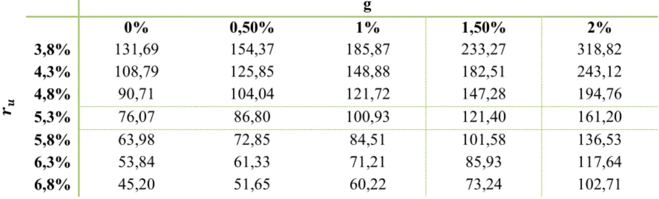
In the next sections, we will explain our assumptions regarding operational flows and discount factors. Moreover, a sensitivity analysis will be presented, in order to understand the magnitude that changes in the discount rate and long-term growth rate may have in the firm value. The currency of this valuation is Euros (€).
Despite having four different segments, they all share the same risks and are influenced by the same key variables. Thus, a single discount rate was computed and used to value the company.
5.1. Explicit period and Terminal Growth Rate
In this valuation, we consider an explicit period of eleven years, from 2016 to 2026. This period finishes with the end of the second DORA, after which we consider the company will be in steady state.
Regarding terminal growth rate, we assumed a 1,5% growth rate, which we consider to be representative of the company reality and in line, even though more conservative, with the consensus of the long-term economy growth, 2%. Thus, we decided to follow the position of more conservative authors, as described in literature (refer to section 2.1.2.2.).
44
5.2. Operational forecasts
5.2.1. Revenues
Aviation segment
For the aviation segment revenues’ forecast, we took into account the two main variables described above, air traffic level and tariffs.
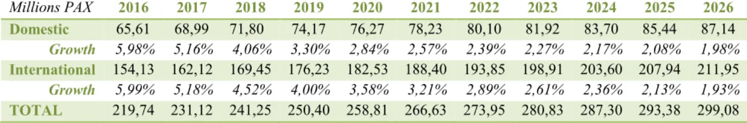
Air traffic is related with GDP behaviour. Taking this into account, we run two regressions (Appendix 8): 1) Relationship between Domestic passengers and the Spanish GDP’s annual changes; and 2) Relationship between International passengers and world GDP’s annual changes; both for the 2000-2014 period.
After, we used the results from the two regressions together with the forecasts of OECD for Spanish and World GDP growth rates in order to reach the expected number of passengers for the foreseeable future. Nevertheless, since this relationship is not linear (passengers are not infinite), a smooth effect was introduced.
2016 2017 2018 2019 2020 2021 2022 2023 2024 2025 2026 Spain 2,35% 2,23% 1,93% 1,73% 1,63% 1,62% 1,66% 1,74% 1,83% 1,93% 2,02%
World 2,74% 2,61% 2,51% 2,44% 2,40% 2,37% 2,35% 2,33% 2,32% 2,30% 2,29%
Table 3: Spain and World GDP's growth rates forecast 2016-2026 (Source: OECD)
Millions PAX 2016 2017 2018 2019 2020 2021 2022 2023 2024 2025 2026 Domestic 65,61 68,99 71,80 74,17 76,27 78,23 80,10 81,92 83,70 85,44 87,14 Growth 5,98% 5,16% 4,06% 3,30% 2,84% 2,57% 2,39% 2,27% 2,17% 2,08% 1,98% International 154,13 162,12 169,45 176,23 182,53 188,40 193,85 198,91 203,60 207,94 211,95 Growth 5,99% 5,18% 4,52% 4,00% 3,58% 3,21% 2,89% 2,61% 2,36% 2,13% 1,93% TOTAL 219,74 231,12 241,25 250,40 258,81 266,63 273,95 280,83 287,30 293,38 299,08
Table 4: Passengers' Evolution: Spanish and International 2016-2026 (Source: OECD; Own calculations)
Regarding tariffs, namely the maximum allowed revenue per passenger, we expect them to maintain their value in 2016 and to be reduced in 2017, since the first DORA will be on place. After 2017, tariffs will remain constant over time.
During the financial crisis, the level of air traffic decreased, which led the regulator to increase tariffs. Nowadays, the economy is recovering and effects were already felt with an increase in passengers’ level. This recovery is expected to continue and, therefore, we expect the regulator to impose a lower limit to the maximum revenue per passenger than the one verified in the previous years.
45 € 2015 2016 2017 2018 2019 2020 2021 2022 2023 2024 2025 2026 Maximum
Revenue/PAX 11,56 11,56 8,46 8,46 8,46 8,46 8,46 8,46 8,46 8,46 8,46 8,46 Table 5: Maximum allowed revenue per passenger 2015-2026 (Source: Own calculations)
In 2012 and 2013, aviation revenue has registered a significant increase, driven by an even larger increase in tariffs. The reduction of domestic passengers has offset partially the tariffs’ increase. On the other hand, in 2017, as tariffs are expected to decrease significantly, aviation revenues will fall. From 2018 onwards, we expect aviation revenues to increase at a moderate level, driven by passengers’ evolution (tariffs are expected to be kept constant).
Commercial segment
For the commercial segment revenues’ estimation, we took into account the passengers’ level evolution. Moreover, we expect international passengers to spend more than domestic ones in commercial areas.
Aena has been implementing a strong strategy to improve commercial revenues, being this one of the main goals of the company for the next years. New contract celebrations with World Duty Free Group and well-known brands as well as constructions to improve commercial areas,
46 moving from traditional stores to walk-through stores, have been showing already some positive financial results. We expect these strategies to maintain their positive impact and, therefore, we believe commercial segment’s revenues will grow, each year, at a rate higher than the total passengers’ growth rate.
Off-terminal services segment
Regarding off-terminal services’ revenues, we forecast them to follow total passengers’ growth rate, meaning that an extra passenger will spend the same amount in off-terminal services than the previous one.
We expect this segment to keep improving its services, maintaining the last years’ efforts in what concerns products offered and service quality.
47 International segment
After Luton Airport full consolidation in Aena’s financial accounts (2014), we expect this segment to maintain a positive evolution year after year, but more moderate.
As reported in the earnings presentation conference call (12/11/2015), the company is not pursuing, currently, any other M&A at an international level, keeping the focus on the current ones.
Luton has a significant impact for this segment and we expect it to continue improving its results, given its importance as the 4th largest airport in London. Therefore, the euro-pound
exchange rate influences the health of the segment. Actually, the company is benefiting from the appreciation of pounds vis-à-vis euros in its financial statements since the consolidation of Luton.
For forecasting purposes, and given the impossibility of estimating exchange rates with accuracy, we based our assumptions in the expected passengers’ level evolution, assuming a constant conversion rate.
48
5.2.2. Operating Expenses
The company has implemented a cost efficiency plan, as described in the previous section, which has proved to be of major success. The sources of inefficiency have now been reduced and, therefore, we forecast operating costs to start increasing again following our air traffic projections.
Since the number of passengers is predicted to increase substantially on the next years, operating expenses are expected to increase with passengers’ growth. In this market, a tariff increase may not be fully reflected in consumers’ bill, since airlines may accommodate part of this increase, passengers should not react a lot to changes in tariffs. For this reason, as Aena intends to keep its service quality - the cost per passenger should remain constant - we decided to forecast the operating expenses’ evolution based on the passengers’ level evolution rather than on the evolution of total revenue (Appendix 9).
Given the impossibility of forecasting impairments of fixed asset disposals, we assumed them to be zero from 2015 onwards.
Graph 17: International revenue 2016-2026 – Drivers (Source: Own calculations)
49 The expected evolution of operating expenses is presented in the following graph. One can conclude that the operating expenses are expected to increase, but at a lower rate as the time goes by.
5.2.3. Operational results
After forecasting both revenues and operating costs, one should analyze the effect that these will have in the profitability of the company. We can do so by analyzing the EBITDA margin, which by excluding depreciations & amortizations allows for a better view of Aena’s profitability. 2016 F 2017F 2018F 2019F 2020F 2021F 2022F 2023F 2024F 2025F 2026F EBITD A Margin 55,2 % 45,4 % 45,6 % 45,6 % 45,6 % 45,7 % 45,7 % 45,8 % 45,8 % 45,9 % 45,9 %
Table 6: EBITDA margin forecast 2016-2021 (Source: Own calculations)
Looking into the table presented above, one can observe that a decline is expected for 2017, explained by the reduction on the aviation segment revenue (given the reduction in the