Emergence of shape and flow structure in Nature in the light of Constructal Theory.

Emergence of shape and flow structure

in Nature in the light of Constructal

Theory

A. Heitor Reis

Physics Department and Évora Geophysics Centre, University of Évora, R, Romão Ramalho, 59, 7000-671, Évora, Portugal

Tel + 351 967324948; Fax: +351 266745394; e-mail: ahr@uevora.pt

1. Introduction

2. Architectures of particle agglomeration 3. Flow architectures of the lungs

4. Scaling laws of river basins 5. Scaling laws of street networks

6. The Constructal Law and Entropy Generation Minimization 7. How the Constructal Law fits among other fundamental principles 8. Conclusion

1.1. Introduction

Constructal theory and the constructal law are terms that we see more and more in the current scientific literature. The reason is that increasing numbers of people use the constructal paradigm to optimize the performance of thermofluid flow systems by generating geometry and flow structure, and to explain natural self-organization and self-optimization. Constructal theory is a principle-based method of constructing machines, which attain optimally their objective. Constructal theory offers a different look at corals, birds, atmospheric flow and, of course, at machines in general.

There is an old history of trying to explain the forms of nature—why does a leaf have nerves, why does a flower have petals—this history is as old as people have existed. Geometry has focused on explaining form, and has contributed to much of the knowledge inherited from antiquity.

For the first time, engineers have entered an arena where until now the discussion was between mathematicians, physicists, biologists, zoologists. The engineers enter with a point of view that is very original, and which may enlighten the questions with which others have struggled until now.

Adrian Bejan is at the origin of the constructal paradigm, which had its start in 1996. In his books [1,2] he tells that the idea came to him when he was trying to solve the problem of minimizing the thermal resistance between an entire heat generating volume and one point. As the optimal solution, he found “a tree network in which every single feature was a result, not an assumption”, and drew the conclusion that every natural tree structure is also the result of optimisation of performance of volume-point flow. As natural tree structures are everywhere, and such structures are not deducible from a known law, he speculated that the optimisation of configuration in time must be a new principle and called it the

constructal law. He stated this law as follows: For a finite-size system to persist in time (to live), it must evolve in such a way that it provides easier access to the imposed (global) currents that flow through it.

A new statement deserves recognition as a principle only if it provides a conceptual framework for predicting form and evolution of form and for modelling natural or engineered systems. Bejan has not only formulated the constructal principle but also developed a method for applying it to practical situations. The

constructal method (Bejan [1-6]) Bejan and Tondeur [7]) is about the generation of

flow architecture in general (e. g. , duct cross-sections, spacings, tree networks). For example, the generation of tree-shaped architecture proceeds from small parts to larger assemblies. The optimal structure is constructed by optimizing volume shape at every

length scale, in a hierarchical sequence that begins with the smallest building block and proceeds towards larger building blocks (which are called “constructs”).

A basic outcome of constructal theory is that system shape and internal flow architecture do not develop by chance, but result from the permanent struggle for better performance and therefore must evolve in time. Natural systems that display an enormous variety of shapes are far from being perfect from the geometric point of view. Geometric perfection means symmetry (e. g., the sphere has the highest possible geometric symmetry) but in the physical (real) world the higher the internal symmetry the closer to equilibrium, to no flow, and death. We know that translational symmetry (invariance) with respect to temperature, pressure and chemical potential means thermal, mechanical and chemical equilibrium respectively, while translational angular invariance of the lagrangian means conservation of linear and angular momentum respectively (Noether’s theorem).

Nevertheless, it is almost impossible to find the perfect geometric form in animate systems because they are far from equilibrium: they are alive, and imperfection (physical and geometrical asymmetry) is the sign that they are alive. Yet, they work “best” because they minimize and balance together the resistances faced by the various internal and external streams under the existing global constraints.

Non-equilibrium means flow asymmetry and imperfection. Imperfection is either geometric (e. g., cylindrical channels, spherical alveolus, quasi-circular stoma, etc.) or physical (unequal distribution of stresses, temperature, pressure, etc.). Therefore, internal imperfections are optimally distributed throughout the system (Bejan [1,2]). The actual form of natural systems that were free to morph in the past is the result of optimal distribution of imperfection, while engineered systems approach the same goal and structure as they tend to optimal performance.

The constructal law is self-standing and distinct from the second law (Bejan [1, 8, 9]). Unlike the second law that accounts for the one-way nature of flows (i.e., irreversibility), the constructal law is about the generation of flow configuration, structure, geometry. Its field of application is that of dissipative processes (flows that overcome resistances), entropy generation, and non-equilibrium thermodynamics. In recent papers, Bejan and Lorente [8, 9] outlined the analogy between the formalism of equilibrium thermodynamics and that of constructal theory (see section 6). In what follows, we outline the main features of constructal theory, and present an overview of recent developments and applications to various fields.

1.2. Constructal method

Constructal theory holds that every flow system exists with purpose (or

objective, function). In nature, flows occur over a wide range of scales with the

purpose of reducing the existing gradients (temperature, pressure, etc.). In engineered and living structures heat and mass flows occur for the same reason, and by dissipating minimum exergy they reduce the food or fuel requirement, and make all such systems (animals, and “man + machine” species) more “fit”, i.e., better survivors. They “flow” better and better, internally and over the surface of the earth.

The purpose of heat engines is to extract maximum useful work from heat currents that flow between systems at different temperatures. Other machines work similarly, i.e. with purpose, e.g. by collecting or distributing streams, or for enhancing heat or mass transfer. Performance is a measure of the degree to which each system realizes its purpose. The design of engineered systems evolves in time towardconfigurations that offer better performance, i.e. better achievement of their purpose.

The system purpose is global. It is present along with fixed global constraints, which may include the space allocated to the system, available material and components, allowable temperature, pressure or stress ranges, etc. The system designer brings together all components, and optimizes the arrangement in order to reach maximum performance. In this way he “constructs” the optimal flow architecture. Therefore, the flow architecture (shape, structure) is deduced, not assumed in advance. Unlike optimising procedures that rely on operational variables, constructal theory focuses on the construction of optimal flow architecture, internal and external.

Optimization makes sense only when purpose exists and the problem-solver has the freedom to morph the configuration in the search of the best solution within the framework of a set of constraints. The constraints may vary from allowable materials, material properties, area or volume allocated to the system, requirements to avoid hot-spots, or not to surpass maximal values of temperature, pressure, stresses, etc. Depending on the system’s nature, optimization may focus on exergy analysis (e.g. Bejan [10, 11]), entropy generation (e.g. Bejan [12, 13]), thermoeconomics (e.g. Bejan et al. [14]) or minimization of highest stress, temperature or pressure (e.g. Bejan [2, 6], Bejan and Tondeur [7]).

The minimization of pressure peaks (Bejan [1, 2, 6], Bejan and Errera [15]) is a good way to illustrate the constructal method. The problem may be formulated as follows:

“A fluid has to be drained from a finite-size volume or area at a definite flow-rate trough a small patch located on its boundary. The flow is volume-point or area-point. It is a special and very important type of flow, because it connects one point with infinity of points. The volume is a non-homogeneous porous medium composed of a material of low permeability K and various layers of higher

permeabilities (K0, K1,..). The thicknesses (D0, D1,…) and lengths (L0, L1,….) of these layers are not specified. Darcy flow is assumed to exist throughout the volume considered. Determine the optimal arrangement of the layers through the given volume such that the highest pressure is minimized.”

A first result is the use of the high permeability material where flow-rates are highest. Conversely, low permeability material shall be used for low flow rates. Next, we choose an elemental volume of length L0 and width H0, filled with the low-permeability (K) isotropic porous medium (e.g. Fig. 1), and use higher low-permeability (K0) material to drain the fluid from it. The area A0=H0L0 of the horizontal surface is fixed but the shape H0/L0 is not.

Because of symmetry and objective (optimization), the strip that collects fluid from the isotropic porous medium must be aligned with the x axis. And, because the flow-rate m&′0 is fixed, to minimize the peak pressure means to minimize

the global flow resistance. The peak pressure occurs in two corners (P, Fig. 1.1), and is given by:

( 0 0 0 0 0)

0

peak m H 8KL L 2K D

P =&′ν + (1)

Fig. 1.1 - Elemental volume: the central high-permeability channel collects flow from low permeability material.

where D0 represents the thickness of the central strip. By minimizing the peak

pressure with respect to the shape parameter H0/L0 we find that the optimum

geometry is described by:

( )

1/4 0 0 2 / 1 0 K ~ 2 H~ = φ − ; 0 1/2

( )

K0 01/4 ~ 2 L~ ₌ − _{φ (2)}

( )

1/2 0 0 0 0 K ~ 2 L H = φ − ; 0 1

( )

K0 0 1/2 ~ 2 P~₌ − _φ − ∆ (3)

where φ0=D0/H0<<1, ∆P~0=Ppeak/(m&0′A0ν/K) and the symbol ~ indicates

nondimensionalized variables based on (A0)1/2 and K as length and permeability scales.

Equations (2) pinpoint the optimal geometry that matches minimum peak pressure and minimum resistance. The first of Eqs. (3) indicates another important result: the two terms on the right hand side of Eq. (1) are equal; said another way, “the shape of the elemental volume is such that the pressure drop along the central strip is equal to the pressure drop along the isotropic porous medium (K layer)”. This is the constructal law of equipartition of the resistances (Bejan [1, 2], Bejan and Tondeur [7]). An analogous result for electric circuits was obtained by Lewins [16] who, based on the constructal theory, found an equipotential division between the competing regimes of low and high resistance currents.

Next, consider a larger volume (a “first construct”) filled entirely with elemental volumes. This “first construct” is shown in Fig. 1.2.

Fig. 1.2 - First construct made of elemental volumes. A new channel of higher permeability collects flow from the elemental volumes.

Once again, symmetry and objective dictate that the higher permeability strip that collects all the currents from the elemental volumes must be aligned with the horizontal axis of the first construct. The geometry of the first construct, namely the number n1 of elemental volumes in the construct, is optimized by repeating the procedure used in the optimization of the elemental volume. If Ci =K~iφi, the parameters defining the optimized first construct are (Bejan [1]):

( )

1/4 0 2 / 1 1 2 C H~ = ; L~1=C0−1/4C11/2 (4)

(

)

1/2 1 0 1 1 L 2C C H = ; ∆P~1=

(

2C0 C1

)

−1/2 (5)

( )

1/2 1 1 2C n ₌ (6)

Higher order constructs can be optimized in a similar way until the specified area is covered completely. What emerges is a two-dimensional fluid tree in which optimization has been performed at every volume scale. The fluid tree is the optimal solution to two problems: the flow architecture that matched the lowest peak pressure, and the one that matched to lowest pressure averaged over the tree.

The constructal law can also be used in the same problem by basing the optimization on minimizing the pressure averaged at each scale of the fluid tree. Three-dimensional fluid trees may be in an optimized analogous manner (Bejan [1, 2, 6]). The same procedure applies to heat transfer trees (Bejan [1-3], Bejan and Tondeur [7], Bejan and Dan [17, 18], Ledezma and Bejan [19]).

1.3. Optimisation as a trade-off between competing trends

There are two competing trends in the example of section 2. Increasing in the length L0 of the central strip leads to a decrease in the resistance posed to flow in the

K layer, but it also increases the resistance along the central channel (cf. Eq. (1)). Optimization meant finding the best allocation of resistances, and therefore the geometry of the system that allows best flow access from the area to the outlet. The law of equipartition of pressure losses summarizes the result of optimization of such flow access.

The optimum balance between competing trends is at origin of “equilibrium” flow architectures in both engineered and natural systems, and is in the domain of constructal theory. Like the thermodynamic equilibrium states that result from the maximization of entropy (or the minimization of free energy) in nonflow systems

in classical thermodynamics, equilibrium flow architectures spring out of the maximization of flow access (Bejan and Lorente [8,9]).

Consider the following example of optimization under competing trends. Air at temperature T0 is made to flow at rate m& through a set of equidistant heat generating boards of length L and width W (perpendicular to the plane of the figure) filling a space of height H (Fig. 1.3).

The board-to-board spacing D, is to be determined in order to maximize the rate q at which heat is removed. As a local constraint, the temperature must not exceed a specified value, Tmax. Other assumptions are laminar flow, smooth board surfaces, and that the temperature along every board is close to Tmax.

Small board-to-board spacings permit a large number of boards (n=H/D) to be installed and cooled. Although in this limit the contact heat transfer area is large, the resistance to fluid flow is also large. The optimal spacing Dopt must come out of the balance between these two competing trends, fluid flow resistance against thermal resistance.

Fig. 1.3 - The optimal spacing comes out of the trade-off between heat transfer surface and resistance to fluid flow. Board to board spacing is optimal when every fluid volume is used for the purpose of heat transfer.

For very small spacings (large n) the heat transfer rate is (Bejan [1]):

(

D2 12

)

(

P L

) (

cp Tmax T0

)

HW

q=ρ µ ∆ − (7)

where ρ, µ and cp stand for density, viscosity and specific heat, respectively. For large spacing (small n), each plate is coated by distinct boundary layers, and the heat transfer rate is given by [1]:

(

)

[

]

(

max 0

)

3 / 1 2 2_{D T T} P L Pr kHW 21 . 1 q= ∆ ρν − (8)

where k, ν and Pr are thermal conductivity, kinematic viscosity and Prandlt number, respectively.

Equation (7) shows that the heat transfer rate q increases asymptotically with

D2 as n becomes smaller (Eq. 7), while when n becomes larger it varies asymptotically as D-2/3 (Eq. 8). Therefore, the number of boards for which the heat transfer rate is maximum can be determined approximately by using the method of intersecting the asymptotes (Bejan [1, 20, 21], as shown in Fig. 1.4.

Fig. 1.4 – The intersection of the asymptotes corresponding to the competing trends indicates the optimum spacing for maximum thermal conductance of a stack of parallel boards.

The optimal spacing is given by: 4 / 1 opt L Be D ∝ − (9)

where Be=(∆PL2)/(µα) is what Bhattacharjee and Grosshandler [22] Petrescu [23]

called the Bejan number.

The spacing defined by Eq. (9) is not only the optimal solution to maximum heat transfer while keeping the temperature below Tmax, but also is the solution to the problem of packing maximum heat transfer rate in a fixed volume. The best elementary construct to this second problem is a heat transfer board whose length matches the entrance length XT (see Fig. 3). Maximum packing occurs when every packet of fluid is used for transferring heat. If L< XT, the fluid in the core of the channel does not interacts thermally with the walls, and therefore does not participate in the global heat transfer enterprise. In the other extreme, L > XT, the flow is fully developed, the fluid is saturated thermally and it overheats as it absorbs additional heat from the board walls.

The optimal spacing determined in this manner enables us to see the significance of the Bejan number. In steady conditions, the rate at which heat is transferred from the boards to the fluid, h(T_max−T₀)WL, must equal the rate of enthalpy increase ρvcp(Tmax-T0)DW, where v=[(∆P)D2]/(12µ), which is removed by the cooling fluid that flows under the pressure difference ∆P. Therefore, for Lopt = XT this equality of scales reads:

(

)

4 opt opt D L D u N 12 Be= (10)

which matches Eq. (9). In Eq. (10), NuD=hD/k=(∂T*/∂z*) is Nusselt number based

on Dopt (where T*=T/(Tmax-T0) and z*=z/Dopt), which is a constant of order 1.

By analogy with section 2, optimized convective heat trees can be constructed at every scale by assembling and optimizing constructs that have been optimized at the preceding scale (Bejan [1], Ledezma and Bejan [19]). Similarity exists between the forced convection results and the corresponding results for natural convection. The role played by Bejan number Be in the forced convection is played in natural convection be the Rayleigh number Ra (Petrescu [23]).

1.4. The ubiquitous search for flow configuration: fields of application of Constructal Theory

Flow architectures are ubiquitous in Nature. From the planetary circulations to the smallest scales we can observe a panoply of motions that exhibit organized flow architectures: general atmospheric circulations, oceanic currents, eddies at the synoptic scale, river drainage basins, dendritic crystals, etc. Fluids circulate in all living structures, which exhibit special flow structures such as lungs, kidneys, arteries and veins in animals, and roots, stems, leaves in plants (Fig.5),

Transportation networks where goods and people flow have been developed on the purpose of maximum access - best performance in economics and for facilitating all human activities. Similarly, internal flow structures where energy, matter and information flow are at the heart of engineered systems.

Flow architectures in both living and engineered systems evolve toward better performance, and persist in time (they survive) while the older disappear (Bejan [1, 24, 25]. This observation bridges the gap between the constructal law and the darwinian view of living systems. Results of the application of constructal theory have been published in recent years for various natural and engineered systems (Reis [25]). In the following, we review briefly some examples of application of constructal theory.

References

[1] A. Bejan, Shape and Structure, from Engineering to Nature, Cambridge University Press, Cambridge, UK, 2000.

[2] A. Bejan, Advanced Engineering Thermodynamics, Second Edition, Wiley, New York, 1997, ch. 13.

[3] A. Bejan, "Constructal-Theory Network of Conducting Paths for Cooling a Heat Generating Volume," International Journal of Heat and Mass Transfer, Vol. 40, 1997, pp. 799-816.

[4] A. Bejan, "Theory of Organization in Nature: Pulsating Physiological Processes," International Journal of Heat and Mass Transfer, Vol. 40, 1997, pp. 2097-2104.

[5] A. Bejan, "How Nature Takes Shape," Mechanical Engineering, Vol. 119, No. 10, October 1997, pp. 90-92.

[6] A. Bejan, "Constructal Tree Network for Fluid Flow between a Finite-Size Volume and One Source or Sink," Revue Générale de Thermique, Vol. 36, 1997, pp. 592-604.

[7] A. Bejan and D. Tondeur, "Equipartition, Optimal Allocation, and the Constructal Approach to Predicting Organization in Nature" Revue Générale de Thermique, Vol. 37, 1998, pp. 165-180.

[8] A. Bejan and S. Lorente “The constructal law and the themodynamics of flow systems with configuration”, International Journal of Heat and Mass Transfer, Vol. 47, 2004, pp. 3203-3214.

[9] A. Bejan and S. Lorente, “Equilibrium and Nonequilibrium Flow System Architectures”, International Journal of Heat & Technology, Vol. 22, No. 1, 2004, pp. 85-92.

[10] A. Bejan, "A Role for Exergy Analysis and Optimization in Aircraft Energy-System Design," ASME AES-Vol. 39, 1999, pp. 209-218.

[11] A. Bejan, “Fundamentals of Exergy Analysis, Entropy Generation Minimization, and the Generation of Flow Architecture”, International Journal of Energy Research, Vol. 26, No. 7, 2002, pp. 545-565.

[12] A. Bejan, Entropy Generation Through Heat and Fluid Flow, Wiley, New York, 1982. [13] A. Bejan, Entropy Generation Minimization, CRC Press, Boca Raton, 1996.

[14] A. Bejan, V. Badescu and A. De Vos, “Constructal Theory of Economics Structure Generation in Space and Time” Energy Conversion and Management, Vol. 41, 2000, pp. 1429-1451.

[15] A. Bejan and M. R. Errera, "Deterministic Tree Networks for Fluid Flow: Geometry for Minimal Flow Resistance between a Volume and One Point," Fractals, Vol. 5, No. 4, 1997, pp. 685-695.

[16] J. Lewins, “Bejan’s constructal theory of equal potential distribution”, International Journal of Heat and Mass Transfer, 46, 2003, pp. 1451-1453.

[17] A. Bejan and N. Dan, "Two Constructal Routes to Minimal Heat Flow Resistance via Greater Internal Complexity," Journal of Heat Transfer, Vol. 121, 1999, pp. 6-14.

[18] A. Bejan and N. Dan, Constructal trees of convective fins”, Journal of Heat Transfer, 121, 1999, pp. 675-682.

[19] G. A. Ledezma and A. Bejan, "Constructal Three-Dimensional Trees for Conduction between a Volume and One Point," Journal of Heat Transfer, Vol. 120, November 1998, pp. 977-984.

[20] A. Bejan, “Convection Heat Transfer” 3rd Ed. 2004, Wiley, New York.

[21] A. Bejan, “Simple Methods for Convection in Porous Media: Scale Analysis and the Intersection of Asymptotes”, International Journal of Energy Research, Vol. 27, 2003, pp. 859-874.

[22] S. Battacharjee and W. L. Grosshandler, “The formation of a wall jet near a high temperature wall under microgravity environment, ASME HTD, 96, 1988, pp. 711-716.

[23] S. Petrescu, “Comments on the optimal spacing of parallel plates cooled by forced convection”, International Journal of Heat and Mass Transfer, 37, 1994, p. 1283.

[24] A. Bejan, "How Nature Takes Shape: Extensions of Constructal Theory to Ducts, Rivers, Turbulence, Cracks, Dendritic Crystals and Spatial Economics," International Journal of Thermal Sciences (Revue Générale de Thermique), Vol. 38, 1999, pp. 653-663.

[25] A. Bejan, “Constructal Theory: An Engineering View on the Generation of Geometric Form in Living (Flow) Systems”, Comments on Theoretical Biology, Vol. 6, No. 4, 2001, pp. 279-302.

[26] A. Heitor Reis, 2006, “Constructal Theory: From Engineering to Physics, and How Flow Systems Develop Shape and Structure”, Applied Mechanics Reviews, Vol.59, Issue 5, pp. 269-282.

2. Architectures of particle agglomeration

2.1. Introduction

The objective of this paper [1] is to bring to the attention of aerosol researchers a new physics principle – the constructal law [2, 3] – the implications of which are general and important in natural, industrial and biological systems [3, 4]. Constructal theory is about the phenomenon of generation of architecture in flow systems. The acquisition of geometry is the mechanism by which the system meets its global objectives under the existing constraints. The objective is the maximization of global access for all the currents that flow through the system. Flow resistances cannot be eliminated. They can be balanced against each other, so that their global effect is minimized. This evolutionary process of balancing and distributing resistances constitutes the generation of flow configuration. The resulting (constructal) configuration is deduced from principle, not assumed, and not postulated.

The global maximization of flow access predicts in simple manner not only the evolution of man-made systems but also the shapes and structures that occur in nature. The rapid development of constructal theory was reviewed by several authors [3 – 7].

In this paper we use constructal theory to describe the morphology of agglomerates of particles.

2.2. Shape and structure of agglomerates of particles

Agglomeration is the process by which particles collide to form larger particles, which typically have greater settling speed. Deposition describes the process by which particles collide and attach to surfaces. Collisions and the coming together of multiple particles result in aggregates that usually have dendritic shape. This pattern of agglomeration and deposition has a profound effect on filtration process, nano-materials processing and the performance of such devices [8, 9].

Agglomerates of aerosol particles often have dendritic shapes that can be observed experimentally [9] or based on numerical simulations [10 – 13]. Is dendritic shape the prevalent and natural form of particle agglomeration? If so, why do aggregates of particles exhibit this particular shape?

[2]. The constructal law requires the architecture of the aggregate of particles to evolve in

time in such a way that the global rate of accumulation of the particles is maximized. The

generation of optimized architectures should bring the entire flow system (ambient + particles) to equilibrium in the fastest way.

Consider the following illustration of why the occurrence of dendritic agglomerates can be anticipated by the constructal law. The forces that make aerosol particles stick onto collectors (filter/beds/previously deposited particles) are of the electrical type. In fact, it is impossible to find electrically neutral surfaces in contact with air. Electrical bonds may occur through interactions of various types (e.g. charge-charge, charge-dipole, dipole-dipole, etc.). However, charge-charge interactions cancel the existing surface charge, and only the charge-dipole interaction ensures a steady and continuing process of deposition, because a dipole-charge bond leaves the total dipole-charge amount invariant (Fig. 2.1).

This is a very common form of interaction because almost all particles have significant dipolar moments.

Assume that a spherical surface with a surface charge density σ collects particles from a surrounding cloud of dipolar particles having uniform concentration C_p in stagnant air.

Before binding to the surface, the small particles travel radially under the influence of charge-dipole forces. For a very small particle travelling with a Stokes flow velocity up, the drag force FD is

c p p D

c

u

d

3

F

₌

πη

(1)

Here η is the dynamic fluid viscosity, dp is the particle diameter and cc is the Cunningham correction factor [8]. The charge-dipole force FC of attraction between the surface and a particle of dipolar moment µr = qra is

3 A 0 C

r

dA

cos

4

1

F

₌

∫

µσ

α

πε

(2)

where ε is the electric permittivity of the air, and r is the distance between the dipole centre and the surface charge (Fig. 2.2). The evaluation of FC may be carried out for the cases of spherical, cylindrical, and planar geometries in the following way:

For spherical geometry, by considering Fig. 2, one has the following relationships:

r sin

θ

= R sin

ϕ

(3)

rcos

θ

+ Rcos

ϕ

= R + h (4)

In order to evaluate the charge-dipole force in the vicinity of the surface we consider

h ~ a/2, sinθ~1. Half of dipolar particles are repelled from the surface while the other half is attracted to the surface. The mean value of cos

α

is 2/

π

. Therefore the mean attractive force between surface charges and dipole (see Eq. 2) reads:

∫

₀0 ₂ 0 Csp sin d R ~ F ϕ

ϕ

ϕ

πε

µσ

(5)

After evaluating the integral in (5) and with sin

ϕ

₀ ~

(

h / R

)

1/2, h ~ a/2, µ=qa, and R=D/2, one has:

1/2 1/2

0

Csp ~ (q ) D

F

_µ

−

πε

σ

(6)

For the cylindrical geometry with cos

ϕ

₀ ~ 1, Eq. (2) reads:

(

)

∫

∫

₋+_∞∞ + 0 0 _{2 2 2} 3/ 2 0 2 Ccy sin R L ) R / L ( d d R 2 ~ F ϕ

ϕ

ϕ

ε

π

µσ

(7) or, with d = R/2 1/2 1/2 0 2 Ccy ~ 2 (q ) d F

_µ

−

ε

π

σ

(8)

Finally, for the force between dipole and planar charged surface one has:

=

∫

₀ /2 2 0 Cpl a d cos sin 2 F π

θ

θ

θ

πε

σµ

(9) or 0 Cpl 3 q 2 F

πε

σ

= (10)

We assume that both forces, FD and FC, cancel each other so that just before

particles bind to the surface they travel with the velocity up. Hence, from Eqs. (1) and (6) we may calculate the flux of particles (n&_sp = C_pu_p / 2, where C_pis the concentration of dipolar particles in the vicinity of the surface) toward the surface of the sphere as 2 / 1 p sp D v K n& = − (11) where

2 / 1 p 0 2 p c p _{(q )} d 6 v c C K

_µ

η

ε

π

σ

= (11a)

By using Eqs. (1) and (8), for a cylindrical surface of diameter d we calculate the flux of particles (n&_cy = C_pu_p / 2) toward the surface as:

2 / 1 p cy d v K 2 n = −

π

& (12)

while, with the help of Eqs. (1) and (10) the flow of particles toward a planar charged surface reads 2 / 1 p pl q v 3 K 2 n _⎟⎟ ⎠ ⎞ ⎜⎜ ⎝ ⎛ =

µ

& (13)

Both spherical and cylindrical modes of agglomeration can occur in nature. The competition between these two modes is the origin of the dendritic shape that occurs throughout nature.

The constructal law requires the architecture of the agglomerate to evolve in time in such a way that the global rate of accumulation of the particles is maximized. The total current of particles (

N

& =

_sp

A

_sp

n

&

_sp), that bind to a spherical surface (area

A

_sp

=

π

D

2) is 2 / 3 p sp

D

v

2

K

N

&

₌

π

(14)

while the total current of particles that bind to a cylindrical surface (length L, area

dL

A

_cy

₌

_π

) is given by: 2 / 1 p cy

Ld

v

K

2

N

&

=

(15)

While from Eq. (13) we see that the flux toward a planar surface depends only on surface charge density and dipole moment, Eqs. (14) and (15) show that the particle binding rate also depends on the geometry of the agglomerate. For the case of a spherical agglomerate we note that

N

&

_sp

=

(

π

2

v

_p

)

D

2

D

&

, and after using Eq. (14) we obtain:

3 / 2 3 / 2

t

2

K

3

D

⎟

⎠

⎞

⎜

⎝

⎛

=

(16)

On the other hand, for a cylinder of fixed length

L

with

N

&

cy

=

(

π

2

v

p

)

Ld

d

&

, we obtain from Eq. (15):

3 / 2 3 / 2

t

K

6

d

_⎟

⎠

⎞

⎜

⎝

⎛

=

π

(17)

Next, we use Eq. (16) to calculate the volume of the spherical agglomerate, 2 2 sp

t

8

K

3

V

₌

π

(18)

Cylindrical growth may develop from a disc, as shown in Fig. 3.

As the diameter increases with time (see Eq. 17) the agglomerate becomes conically shaped (Fig. 2.3). In this case the growth speed along the axis is given by

L

& =

n

&

_pl

v

_p. Then, by using Eq. (13) we obtain

2 / 1

q

3

K

2

L

⎟

⎠

⎞

⎜

⎝

⎛

=

µ

&

(19)

Using Eqs. (17) and (19) and integrating with respect to time, we find the volume of the conically shaped agglomerate

3 / 7 2 / 1 3 / 1 co

(

Kt

)

q

6

7

3

V

⎟

⎠

⎞

⎜

⎝

⎛

⎟

⎠

⎞

⎜

⎝

⎛

=

µ

π

(20)

From Eqs. (18) and (20) we see that the ratio 3 / 1 2 / 1 3 / 1 co sp

t

q

K

2

.

2

V

V

₋

⎟⎟

⎠

⎞

⎜⎜

⎝

⎛

=

µ

(21)

is initially very high, and that it approaches 0 as t becomes sufficiently large. According to the constructal law this means that the agglomerate first must grow as a sphere, and change to the conical shape at a critical time later in its development. From Eq. (21) we see that for

2 / 3

q

K

9

.

9

t

_⎟⎟

⎠

⎞

⎜⎜

⎝

⎛

>

µ

(22)

the conically shaped agglomerate is more efficient as a particle collector than the spherically shaped agglomerate.

For water nucleating in ambient air, K is of order 10−11m3/2s−1(which corresponds to a surface/water vapor field of order 10−2 µV m-1) and

( )

1/2 4

10 ~

q −

µ m. Therefore, the critical time for switching between spherical and conical growth as a preferential mode of agglomeration is of order 1 s, which corresponds to D ~ 10-7 m for the diameter of the agglomerate. It is also interesting to compare the growth speeds of cone diameter and cone tip. By using Eqs. (17) and (19) we obtain: 3 / 1 2 / 1 3 / 1 t q K 36 L d ₋ ⎟⎟ ⎠ ⎞ ⎜⎜ ⎝ ⎛ ⎟ ⎠ ⎞ ⎜ ⎝ ⎛ =

µ

& & (23)

which decreases as t−1/3 . This means that at later stages the agglomerate grows as a needle, the geometry of which is obtained from Eqs. (17) and (19) (Fig. 3)

2/3 3 / 1 3 / 2

L

q

9

d

_⎟⎟

⎠

⎞

⎜⎜

⎝

⎛

⎟

⎠

⎞

⎜

⎝

⎛

=

µ

π

(24)

As an example, dendritic snow crystals have a length scale of order 10-3 m, and, by taking into account Eq. (24), we find

d

/

L

~

10

−2

L

−1/3 , which for L ~ 1 mm yields d/L ~ 10-2. This agrees with the order of magnitude of the diameter/length ratio of snowflake needles. Moreover, following Eq. (19) the needle tip growth speed is constant in accordance with experimental results [18].

One interesting aspect of the geometry predicted in Eq. (24) is that it depends only on the dipole moment

µ

. This means that weakly dipolar molecules will

agglomerate in a needle that is more slender than the needle formed by strongly dipolar molecules.

Another noteworthy aspect is that the critical time for switching from spherical to needle shaped growth depends only on the dipole strength, cf. Eq. (24). From Eqs. (16) and (22) we calculate the critical diameter of the original sphere as

a

6

~

q

6

~

D

_crit

µ

(25)

This means that a universal behaviour of particle agglomeration exists: when the sphere diameter reaches 6 particle diameters, the agglomerate (of

113 ~ 6 ) 6 /

(π × 3 particles) must switch from spherical to needle-shaped growth as a preferential mode of particle agglomeration.

Secondary needles may grow from specific points of the needle surface, generating in this way dendritic-growth architectures. A heat diffusion mechanism for explaining dendritic growth in snowflakes was proposed in [3].

In summary, the constructal law enables us to predict important features of shape generation and architecture of particle agglomeration. In the very beginning the agglomerate grows as a sphere, because at short times this shape is more effective in collecting particles from the environment.

There are many natural flow systems for which the architecture was proven to be optimized in accordance with the constructal law. Examples include the respiratory tree [15], river basins [5, 6], bacterial growth [5], patterns of cracks on the ground [3], and dendritic crystal growth [3, 16].

2.3. Concluding remarks

We showed that structure of particle agglomeration is generated in the pursuit of the equilibrium in the fastest way (constructal law) i.e., trough the maximization of particle agglomeration rate. At small times, spherical agglomeration of particles around a particle collector is the most effective mechanism. After a critical time the configuration switches from spherical symmetry to needle-shaped agglomeration, which performs best as a particle collector at long times. Secondary needle developments give rise to dendritic patterns. It was shown that the shape of the needle depends on the dipolar moment of the particles and that the critical number of particles in the spherical agglomerate before switching to needle shape does not

depend on the particle properties.

Nomenclature

a – spacing between charges (dipole), m A – area, m2

B – pressure drop number cc – Cunningham factor

C – concentration, kg m-3

d – diameter of cylinder or distance, m

d& – speed of diameter growth, m s-1 D – diameter of sphere, m Ddf – diffusion coefficient, m2s-1 Dh – hydraulic diameter, m F – force, N H – height, m K – constant (Eq. 11), m5/2 s-2 L – length, m

L& – speed of needle tip growth, m s-1

m – particle transfer density, kg m-3 s-1 n& – flux of particles, s-1 m-2

N& – current of particles, s-1 p – pressure, Pa P0 – Poiseuille number q – charge, C Re – Reynolds number Sc – Schmidt number Sh – Sherwood number t – time, s U – velocity, ms-1 V – volume, m3

H, L, W – height, length, width, m Z – wetted perimeter, m Greek Symbols α, ϕ, θ – angle, rad ε – porosity ε0 – electric permittivity, C2 N-1 m-2 φ – number of tubes/plates η – viscosity, N s m-2 κ – permeability, m2

λ – particle transfer coefficient, ms-1 µ – dipole moment, C m

ρ – air density, kg m-3

σ – surface density of charge, C m-2

τ – shear stress, Nm-2 Subscripts C – charge/dipole cy – cylinder D – drag op – optimized p – particle pl – plane References

[1] A. H. Reis, A. F.Miguel, and A. Bejan, 2006, , Journal of Physics D: Applied Physics, 39, 2311-2318

[2] A. Bejan, Advanced Engineering Thermodynamics, chapter 13, 2nd edn. (Wiley, New York, 1997).

[3]A. Bejan, Shape and Structure, from Engineering to Nature (Cambridge University Press, Cambridge, 2000).

[4] A. Bejan, I. Dincer, S. Lorente, A. F. Miguel and A. H. Reis, Porous and Complex Flow Structures in Modern Technologies (Springer, New York 2004).

[5] R. N. Rosa, A. H. Reis and A. F. Miguel, Bejan's Constructal Theory of Shape and Structure (Ed. University of Evora, Center of Geofisica of Evora, Portugal, 2004).

[6] A. H. Reis, 2006 Geomorphology, Vol. 78, 201-206.

[7] A. H. Reis, 2006, , Applied Mechanics Reviews, Vol.59, Issue 5, pp. 269-282. [8] O. Filippova and D. Hänel, Journal of Aerosol Science 27, S627 (1996)

[9] M. J. Lehmann and G. Kasper, in Proceedings of the International workshop on particle loading and kinetics of filtration in fibrous filters (Institut für Mechanische Verfahrenstechnik und Mechanik, Universität Karlsruhe, Germany, 2002).

[11] C. Kanaoka, in Advances in Aerosol Filtration, edited by K. R. Spurny (CRC Press LCC. Washington, 1998), p. 323.

[12] R. Przekop, A. Moskal and L. Gradon, Journal of Aerosol Science 34, 133 (2003). [13] O. Filippova and D. Hänel, Computers and Fluids 26, 697 (1997).

[14] K. G. Libbrecht, Rep. Prog. Phys. 68, 855 (2005).

[15] A. H. Reis, A. F. Miguel and M. Aydin, Medical Physics 31, 1135 (2004). [16] A. Bejan, Revue Générale de Thermique 38, 653 (1999).

3. Flow architecture of the lungs

3.1 Introduction

The Constructal Principle that has been originally formulated by Adrian Bejan states that every system with internal flows develops the flow architecture that maximizes the heat and mass flow access under the constraints posed to the flow. In all classes of flow systems (animate, inanimate, engineered) the generation of flow architecture emerges as a universal phenomenon. This has been shown in a number of articles by Bejan and is summarized in a recent book [1].

By using the Constructal Principle, Bejan has addressed the rhythm of respiration in animals in relation with the body size and found that the breathing time increases with the animal body size rose to a power of 1/4, which is in good agreement with the biological observations.1 A number of other recent studies have focused either on the characteristics of the airflow and gas diffusion within the lungs [2-6] and the form of the arterial bifurcations [6, 7] or statistical description of the respiratory tree [8,9].

In this work [15] we focus on the structure of the pulmonary airflow tree. The respiratory system is basically a fluid tree that starts at the trachea and bifurcates 23 times before reaching the alveolar sacs [4, 10] The reason for the existence of just 23 bifurcations in the respiratory tree (Fig. 3.1) has remained unexplained in the literature. Has this special flow architecture been developed by chance or does it represent the optimum structure for the lung’s purpose, which is the oxygenation of the blood? The view that the Constructal Law which has been originally developed for engineered systems, holds also for living systems will guide us in finding the best airflow architecture for the respiratory system.

3.2 A fluid tree with purpose

The oxygenation of blood takes place in the tissues that shape the surface of the alveolar sacs. High alveolar surface promotes better oxygenation, but requires increased access to the external air. In fact, if the access to the external air faces high flow resistance the rate of oxygen diffusion into the blood is lowered due to the poor oxygen concentration in the air within the alveolar sacs.

Fig. 3.1 Model of the respiratory tree with trachea, 23 bronchial bifurcations and alveolar sacs.

According to the Constructal Law a fluid tree that performs the oxygenation of blood and removal of carbon dioxide at the lowest flow resistance should exist under the constraints posed by the space allocated to the respiratory process. This fluid tree should be able to promote the easiest access to the external air. Two possibilities exist for accomplishing this purpose: (I) a duct system that ends with an alveolar volume from which the oxygen diffuses to the tissues, where it meets the blood, and in which the carbon dioxide diffuses after being released from the blood, or (II) a unique volume open to the external air, in which the oxygen reaches the blood in the tissues, and removes the carbon dioxide rejected from the blood, only by

diffusion through the internal air.

This second possibility is clearly non-competitive as compared to the first. The access time for a diffusive process between the entrance of the trachea and the alveolar sacs at a distance L~5×10-1

m is tdiff =L2/D ~104 s, where D ~2×10-5 m2/s is the diffusion coefficient for oxygen in air. The access time for duct flow is of order tflow= πηL2/(D02∆P )~1 s, where D0 ~10-2 m is the trachea diameter, η ~2×10-5 Ns/m2 is air dynamic viscosity, and ∆P~1 Pa is the scale of the average pressure difference.

Therefore the channeling of the air from the outside to the alveolar surface enables better performance of the respiratory process.

However, a cavity (or alveolar sac) at the end of the channeling tree must exist, as the oxygenation of the blood occurs by diffusion from air into the tissues. Oxygen diffusion is proportional to the alveolar surface that, in turn, is proportional to the number of bronchioles corresponding to the final level of bifurcation, which is

2N, N being the number of bifurcation levels. On the other hand, the higher the

number of alveolar sacs is, the higher the complexity gets as well as the flow resistance of the duct network. Therefore, the optimum flow structure must emerge from the minimization of the overall resistance, i.e. the duct resistance plus the diffusive resistance.

3.3 Bronchial tree resistance and alveolar resistance

Oxygen and carbon dioxide flow within the respiratory tree (bronchial tree plus alveolar sacs) under several driving forces. So as to evaluate and compare the flow resistances we will express the flow rates in terms of a unique potential. Airflow within the bronchial tree is assumed to be laminar, isothermal and incompressible. As this flow is also adiabatic, i.e. ∆s=0, conservation of total energy

per unit mass that is the sum of internal energy, u =-P/ρ+Ts+µ (where P is pressure, ρ is density, T is temperature, s is entropy and µ is chemical potential) plus kinetic energyε , along the respiratory tree, implies:

ε ∆ ∆ ρ µ ∆ = −1 _P+ ₍₁₎ Oxygen and carbon dioxide are assumed to be in equilibrium with the air that flows within the bronchial tree, which means that all gases in the airflow have the same chemical potential and move as a whole between the entrance of the trachea and the alveolar sacs. In this way, the airflow is driven by the gradient of the

chemical potential within the bronchial tree, which in each duct is related to the pressure gradient by Eq. (1) as ∆µ=ρ−1∆P_{. Hence, by considering the bronchial tree}

as composed of cylindrical channels and assuming Hagen-Poiseuille flow, the airflow rate is determined by

_cn n 4 n n ₁₂₈D_L m _∆µ ν πρ = & (2)

where m& and _n ∆µcn stand for airflow rate and chemical potential difference between the ends of a channel at the nth bifurcation level, respectively, and ν is the air

kinematic viscosity. For laminar flow the minimum flow resistance at a bifurcation is achieved if the ratio between consecutive duct diameters is [12,14]:

Dn/Dn-1=2-1/3 (3) and if the ratio of the respective lengths, Li , is

Ln/Ln-1=2-1/3 (4) Eqs. (3) and (4) represent constructal laws that hold for consecutive channels at a bifurcation. They are robust in the sense that hold for any bifurcation angle [12-14] and express the empirical relation known as Murray’s law. Taking into account Eqs. (3) and (4), the resistance to laminar flow posed by the nth bronchial tube is

₄ 0 0 n n cn cn D L 128 2 m r πρ ν µ ∆ ₌ = & (5) where D0 and L0 are the diameter and the length of the first tube in the tree i.e. the trachea, respectively.

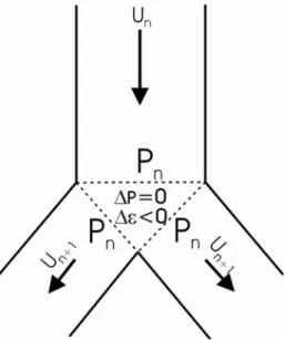
Each bifurcation implies an additional resistance to airflow. In the derivation of Eq. (2) it has been assumed that pressure has no radial variation along each channel. Such a condition implies that in a bifurcation the variation of the chemical potential is entirely due to the variation in the kinetic energy, as shown in Fig. 3.2 Therefore considering Eq. (1) the airflow rate in a bifurcation may be described by: bn bn bn bn n _{r r} m& =∆µ =−∆ε (6) where ∆εbn is the variation of the average kinetic energy per unit mass in the bifurcation. Taking into account the velocity (U) profile of cylindrical Hagen-Poiseulle flow, the variation of the kinetic energy per unit mass that flows trough a

Fig. 3.2 Hagen-Poiseille flow in a bifurcation. The resistance to airflow is due to the variation of the average kinetic energy per unit mass, and proportional to the mass flow rate.

bifurcation is calculated as ∆ε =(ρ/m&_n)

(

2

∫

_n+1U3dA−

∫

_nU3dA

)

, together with Eqs. (2)-(4), gives the airflow resistance in a bifurcation in the form:

₄ n/3 0 20 bn 2 D 8 m r πρ & = (7) where m& represents the airflow rate in the trachea. In this way, with the exception ₀ of the channels that connect to the alveolar sacs, every other channel may be viewed as having a Hagen-Poiseulle type resistance given by Eq. (5) plus a resistance at the end due to bifurcation given by Eq. (7).

If ∆µ_n =∆µ_cn +∆µ_bn denotes the total variation of the chemical potential in channels in the nth level of bifurcation (n=0, for the trachea), from Eqs (5) and (7) and taking into account that in this level there are 2n bronchial tubes, we obtain the total resistance of the nth level as

_⎟⎟ ⎠ ⎞ ⎜ ⎜ ⎝ ⎛ + = − 0 3 / n 2 0 4 0 0 n 1 m₁₀₂₄2 _L D L 128 r ρν πρ ν & (8)

Then, the overall convective resistance of a tree with trachea (n=0) plus (N-1) bifurcation levels is given by

(

)

⎥ ⎥ ⎦ ⎤ ⎢ ⎢ ⎣ ⎡ ₋ + = = − − =

∑

0 3 / N 2 0 4 0 0 1 N 0 n n B N m ₃₇₉1 2 _L D L 128 r R πρν πρ ν & ₍₉₎

For a normal breathing frequency of 12 times per minute and tidal air of about 0.5 dm3 we conclude that m&₀

(

1−2−2N/3

)

(379πρνL₀)<<1, and this term that corresponds to the sum of airflow resistances in the bifurcations may be neglected in Eq. (9).

If (φox)0 and φox denote the average relative concentration of the oxygen in the air at the entrance of the trachea and at the bronchial tree, respectively, the average oxygen current towards the interior of the bronchial tree is

[

( )

]

( )

ox _B b b ox 0 ox ox ₂1 m _R m& = _φ −_φ & = ∆µ (10) where the subscript ox means oxygen. In Eq. (10) the factor 1/2 arises because either inhaling or exhaling last half of breathing time, ∆µ_B =

∑

N_n=−₀1∆µ_N is the absolute value of the variation of the chemical potential of the air in the trachea plus the

(N-1) levels of bifurcation, and

( )

R_{ox B} =2R_B/

(

( )

φ_{ox 0} −φ_ox

)

is the resistance to oxygen transport.

However, no such equilibrium conditions exist between the components of the air within the alveolar sacs, because the chemical potential of oxygen in the alveolar tissues is lower than that in the alveolar air, while the chemical potential of carbon dioxide in the tissue is higher than that in the alveolar air. Therefore oxygen diffuses from the alveolar air into the tissues, while carbon dioxide diffuses in the opposite direction. It is assumed that oxygen diffuses at the 2N alveolar sacs according to Fick’s law, consequently the total oxygen current to the alveolar sacs, which are considered to be in a spherical shape with diameter d and total area πd2

(see Fig. 3), is given by

=

∫

0

(

)

2 a ox ox N ox ₂ d sin d D 2 m _π δ θ θ π ρ ∆ & (11)

where Dox is the oxygen diffusivity, (∆ρox)a is the difference between the oxygen concentrations at the entrance of the alveolar sac and the alveolar surface, and

2 / ) cos 1 ( d _θ

δ = − , (see Fig. 3.3). Taking into account that

(

_∆ρox

)

_a =_φoxρ

(

_∆µox

)

_a /

( )

R_{g ox}T , where (Rg)ox=R/Mox is the gas constant for oxygen and φox is the relative concentration of oxygen in the alveolar air, and assuming that

the chemical potential of oxygen does not vary over the alveolar surface, integration of the r.h.s. of Eq. (11) yields:

(

)

( )

R T D d 2 2 m ox g a ox ox ox N ox = π ρφ ∆µ & (12)

The diameter of the alveolar sac may be determined as the difference between the overall lengths L, of a bronchial tree with infinite bifurcations, which is the limiting length defined by the constructal law, Eq. (4), and that of the actual tree with N bifurcation levels, i.e.

∑

= − = N 1 i i L L d (13)

The length LN of a tree with N bifurcations may be determined from Eq. (4) as the length of the trachea plus the lengths of the N consecutive bronchioles is given by the sum of N + 1 terms of a geometric series of ratio 2-1/3 as:

_{1/3 0} 3 / ) 1 N ( N 0 i i L 2 1 2 1 L − ₋+ = − − =

∑

(14) Therefore,

∑

= ∞ → = N 0 i i L L lim

N , namelyL=4.85L0. Eqs. (13) and (14) enable us to determine the diameter of the alveolar sac as

d =4.85×2−(N+1)/3L₀ (15) In consequence, Eq. (12) may be written as

_{( )}

(

_ox

)

_a ox g 3 / N 2 ox ox 0 ox 7.70 L D _R2 _T m& = _{π φ ρ ∆µ} (16)

Fig. 3.3 Model of the respiratory tree with a conductive part (bronchioles) and a diffusive space (alveolar sac)

In this way, the resistance of the Nth level of bifurcation that is the sum of the convective resistance of the last 2N channels, which is given by 2-NrcN (see, Eq. (5)), plus the alveolar diffusive resistance given by Eq. (16), (see also Eq. (10)) is

( )

( )

[

]

( )

ox 0 ox 3 / N 2 ox g 4 0 ox 0 ox 0 N ox 0.13R T 2 _{L D} D L 128 R ρ πφ ρ φ φ π ν ₊ − − = (17)

Therefore, if _∆µox =(_∆µox)_B +(_∆µox)_N +(_∆µox)_a is the total difference between chemical potential of the oxygen in the external air and the oxygen close to the alveolar surface, the total resistance,R_ox =∆µ_ox /m&_ox, posed to oxygen as it moves from the external air into the alveolar surface, which is the sum of the resistance (Rox)B, given by Eq. (9), with (Rox)N given by Eq. (17), reads:

( )

[

_{φ φ}

]

_ρ π

( )

φ ρ π ν ox ox 0 3 / N 2 ox g ox 0 ox 4 0 0 ox _{L D} 2 T R 13 . 0 ) 1 N ( D L 256 R − + + − ≅ (18)

where the resistances in the bifurcations have been neglected due to the fact that its value is very small as compared to channel resistances. The total resistance is composed of a convective resistance and a diffusive resistance represented by the first and the second terms of the r.h.s of the Eq. (18), respectively.

3.4 Optimisation of the respiratory tree based on the Constructal Law

According to the Constructal Law the flow architectures evolve in time in order to maximize the flow access under the constraints posed to the flow. We believe that, during millions of years of human evolution, the oxygen-access performance of the respiratory tree was optimized naturally, through changes in flow architecture.

In Eq. (18), the convective part of the resistance increases as the number of bifurcations increases, while the diffusive resistance decreases. The number of bifurcations is the free parameter that can be optimized in order to maximize the oxygen access to the alveolar surface or, in other words to minimize the total resistance to oxygen access.

The average value of oxygen relative concentration within the respiratory tree, φox, may be evaluated from the alveolar air equation in the form: ((φox)0-φox

)Q-S=0, where (φox)0 ~1/2(φair+φox) and φair are the oxygen relative concentration at the entrance of the trachea, and in the external air, respectively, Q is the tidal airflow

and S is the rate of oxygen consumption. With φair=0.2095, Q~6 dm3/min and S~0.3 dm3/min [5,11] we obtain φox ~ 0.1095.

For L0 we take the sum of the larynx and trachea lengths (first duct), which is typically 15 cm, while the trachea diameter, D0, is approximately 1.5 cm [10,11). Air

and oxygen properties were taken at 36º C, namely ν = 1.7×10-5 m2/s, Dox = 2.2×10 -5

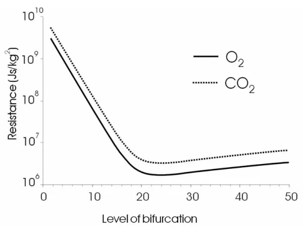
m2/s, (Rg)ox=259.8 J/(kg.K), The plot of the total resistance of the respiratory tree against the bifurcation level is shown in Fig. 3.4. In can be seen that the minimum is flat and occurs close to N=23.

A more accurate value of this minimum is obtained analytically from Eq. (18). The optimum number of bifurcation levels is given by

( )

( )

⎥ ⎥ ⎦ ⎤ ⎢ ⎢ ⎣ ⎡ ⎟⎟ ⎠ ⎞ ⎜⎜ ⎝ ⎛ − × = − 1 D L T R D 10 35 . 2 ln 164 . 2 N ox 0 ox ox 2 0 ox g 4 0 4 opt φ_φ ν (19)

which yields N_opt =23.4. As N must be an integer, this means that the optimum number should be 23.

Fig 3.4 Total resistance to oxygen and carbon dioxide transport between the entrance of the trachea and the alveolar surface is plotted as function of the level of bifurcation (n). The minimum resistance both to oxygen access and carbon dioxide removal corresponds to N=23.

In view of the simplifications of the model (mainly the geometry of the bronchial tubes which are assumed to be cylindrical and the geometry of the alveolar sacs which are viewed as spheres, this result is in a very good agreement with the literature, which indicates 23 as the number of bifurcations of the human bronchial tree [4,10].

The respiratory tree can also be optimized for carbon dioxide removal from the alveolar sacs. In this case the correspondent equation to Nopt is Eq, (18) with r.h.s multiplied by –1 and the correspondent values of the diffusion coefficient, which is

Dcd=1.9×10-5m2/s for carbon dioxide, the gas constant (Rg)cd=189 J kg-1 K-1, and the value of the average relative concentration of carbon dioxide in the respiratory tree, φcd=0.04. In the calculation of φcd we used S=0.24dm3/min since the respiratory coefficient is close to 0.8 and (φcd)air ~ 0.315×10-3. The plot of the resistance to carbon dioxide removal against bifurcation level is shown in Fig. 4. The minimum resistance, as calculated from Eq. (18), corresponds to Nopt = 23.2.

We can say that the human respiratory tree, with its 23 bifurcations, is optimized for both oxygen access and carbon dioxide removal. For N=23 the resistance to carbon dioxide removal is 4.8×106

J s kg-2 and higher than the resistance to oxygen access that is 2.60×106

J s kg-2.

One of the initial assumptions of this model of respiratory tree was that diffusion can be neglected within the bronchial tree where oxygen is transported in the airflow while diffusion is the main way of oxygen transport in the alveolar sacs. By using Eq. (2) and considering tidal volume of 0.5 dm3, breathing frequency of 12 times per minute and trachea diameter of 0.015 m, we calculate the average velocity of the airflow, and therefore of the oxygen current, in the last bronchiole before the alveolar sac, which is of order 6mm/s. On the other hand, the average velocity of the diffusive current of oxygen in the alveolar sacs is of order Dox/2πd ~1.3 mm/s. These results are consistent with the initial assumptions of the model. However, as in this idealized model the velocities of the oxygen for convective and diffusive current simply approach each other, in the real respiratory tree we can expect that in some branches they are of the same order, what indicates the possibility of developing alveoli before the end of the bronchial tree as really happens in the human respiratory tree [5].

If the number Nopt=23 is common to mankind then a constructal rule emerges from Eq. (19): “the ratio of the square of the trachea diameter to its length is constant and a

length characteristic of mankind”

const. 1.5 10 m L D ₃ 0 2 0 _{= = ×} − = λ (20) This number has a special relationship with some special features of the space allocated to the respiratory process as we show next. From Eqs. (3) and (4) we can estimate the volume occupied by the bronchial tree, which is the sum of the volumes of the 23 bifurcation levels, as VB=23×(π/4)D02L0. The total volume of the alveolar sacs is V=223(π/6)d3. We see that VB/V<<1, which means that the volume of the lungs practically corresponds to the volume, V, occupied by the alveolar sacs. The internal area of the alveolar sacs is A=223×πd2, and therefore A/V=6/d. By using the Eqs. (14), (15) which lead to L=2(N+1)/3d, together with Eq. (18) we obtain the following relationship:

_{( )}

[

]

2 / 1 ox 0 ox ox g ox ox 0 2 0 ) ) ( T R D V AL 63 . 8 L D ⎪⎭ ⎪ ⎬ ⎫ ⎪⎩ ⎪ ⎨ ⎧ − = φ φ φ ν ₍₂₁₎ The non-dimensional number AL/V, determines the characteristic length λ=D02/L0, which determines the number of bifurcations of the respiratory tree by Eq. (19). This constructal law is formulated as follows: “The alveolar area required for gas

exchange, A, the volume allocated to the respiratory system, V, and the length of the respiratory tree, L, which are constraints posed to the respiratory process determine univocally the structure of the lungs, namely the bifurcation level of the bronchial tree.”

From Eq. (14), we obtain L=4.85L₀=0.73m for the total length of the respiratory tree and from Eq. (21) we obtain d=6V/A=2.86×10-3

m. Therefore we have the alveolar surface area as A=223πd2 =215.5m2 and the total alveolar volume

V=223(π/6)d3 =102.7dm3. The alveolar surface area A, is not much far from the values found in literature that fall in the range 100-150m2. However, the value found for the total alveolar volume is much higher than the average lung capacity (~7.5 dm3). This may arise from lung’s volume being calculated as the alveolar sacs were fully inflated. Nevertheless, the value found for total alveolar volume suggests that the dimension of the alveolar sacs was somehow overestimated.