Equity Valuation
The Linde Group
Master Thesis
Submitted to: José Carlos Tudela Martins Católica-Lisbon: School of Business and Economics
Master of Science in Finance
10.03.2014
Manuel Lorenz
Acknowledgements
Writing this thesis was a hard exercise for myself. It demanded a lot of dedication, attention to detail and the application of the knowledge I obtained during my studies. Nevertheless, at the end it was a very satisfying experience and with all the effort I put into it I am finally happy with the result.
I enjoyed working on this thesis, not only because of the topic itself, and I want to thank some people who supported me during this challenging period. First to mention is professor José Carlos Tudela Martins. I want to thank you for the uncomplicated way you enabled me to write this thesis and the immediate support you gave me everytime it was needed. You answered all of my questions quickly and precisely which enabled me to solve several problems I had when writing this thesis. I also want to thank my former classmate, roommate and friend Benedikt Popp for always talking to me when I had doubts and for supporting me in every aspect he could. I also want to thank my girlfriend Verena Kapfer. You didn’t give me the professional input, but sometimes the personal support is way more important than anything else. And finally, I want to thank my parents for supporting me through all my studies from the beginning to the end.
Abstract
This analysis provides a stock valuation of The Linde Group, a Germany based Industrial Gases company and one of the main players within this industry worldwide. After reviewing the most recent literature in terms of valuation, two different methods, namely the DCF Valuation and the Multiple Approach, are applied to determine the enterprise- and equity value of the company. Further insights are provided through a sensitivity analysis, giving more information about the main drivers for the obtained valuation of Linde. Finally, the results are compared to the estimations of Morgan Stanley, summarizing and explaining the main differences and their origins.
Table of Content
1. Introduction ... 1
2. Literature Review... 2
2.1 The Discounted Cash Flow Valuation Models ... 2
2.1.1 Free Cash Flow ... 3
2.1.2 Terminal Value ... 5
2.1.3 Cost of Capital Calculation ... 7
2.2 The Multiple Approach ... 13
2.3 The Option Based Valuation ... 16
3. Company Overview and Market Analysis ... 16
3.1 The Linde Group ... 16
3.1.1 Historical Background ... 16
3.1.2 Organizational Structure and Product Overview ... 17
3.1.3 Strategic Focus ... 19
3.1.4 Stock Information ... 23
3.2 The Industrial Gases Industry ... 25
4. Valuation ... 27
4.1 Historical Data Analysis ... 28
4.1.2 Income Statement – Historical Performance Overview ... 34
4.1.3 Historical Performance Summary... 39
4.2 Discounted Cash Flow Valuation ... 39
4.2.1 Income Statement Forecast ... 40
4.2.2 Balance Sheet Estimations ... 52
4.2.3 Valuation Model Inputs ... 55
4.3 Multiple Valuation ... 66
4.4 Sensitivity Analysis ... 68
5. Valuation Analysis’ Results in Comparison to Morgan Stanley’s Estimations ... 74
6. Conclusion ... 76
Appendices ... 78
List of Appendices
Appendix 1: The Fama French Three Factor Model ... 78
Appendix 2: The Arbitrage Pricing Theory ... 79
Appendix 3: Linde Customer Overview ... 79
Appendix 4: Net Cash Position ... 80
Appendix 5: Traded Bonds Overview ... 80
Appendix 6: Market Value of Debt Calculation Formula ... 80
Appendix 7: Morgan Stanley Valuation Overview ... 81
Appendix 8: Linde Dividend Payout Ratio 2008 – 2012 ... 81
Appendix 9: GDP by Countries and Reportable Segments (2010 – 2018) ... 82
Appendix 10: Industrial Production Forecast Regression Analysis by Regions ... 84
Appendix 11: Long-Term Global GDP Forecast ... 85
Appendix 12: Equity Risk Premium by Countries ... 86
Appendix 13: Financial Debt Maturity Profile ... 87
Appendix 14: Non-Abbreviated Income Statement ... 88
Table of Figures
Figure 1: Linde Organizational Structure ... 18
Figure 2: Gas and Oil Demand Comparison by Geographies between 2011 and 2025 ... 21
Figure 3: Capital Expenditure in Emerging and Developed Markets in €m ... 22
Figure 4: Expected Cost Savings by Segments ... 23
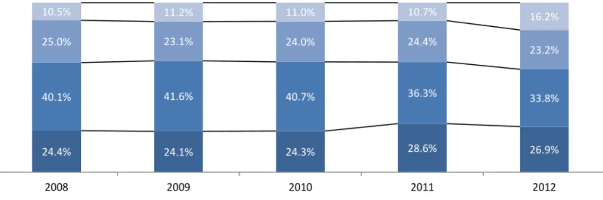
Figure 5: Linde Shareholder Structure by Regions ... 24
Figure 6: Linde and DAX 30 Historical Price Developments from 2007 – 2014 in € ... 25
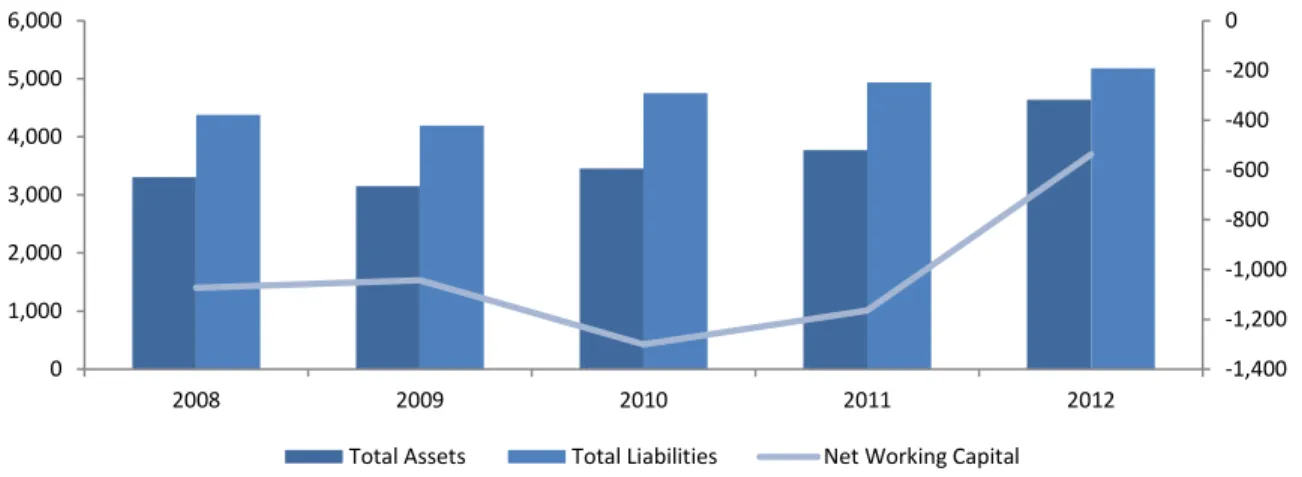
Figure 7: Net Working Capital (2008 – 2012) ... 33
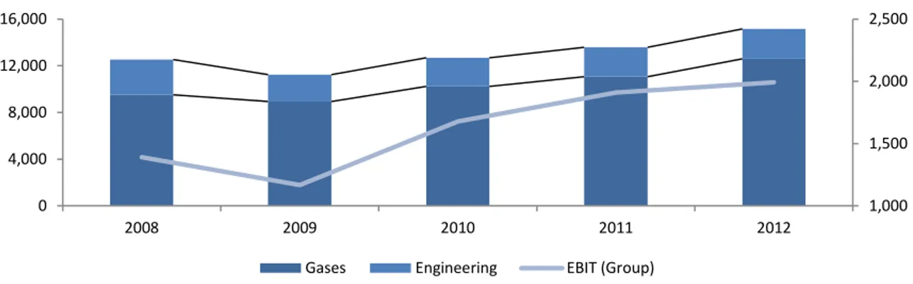
Figure 8: Revenue Development by Division and Group EBIT (2008 – 2012) ... 34
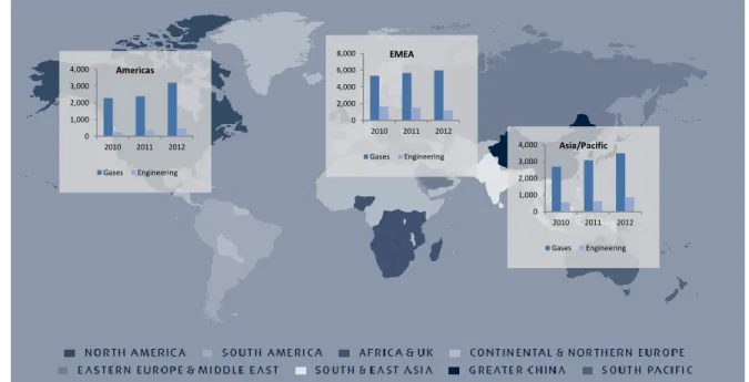
Figure 9: Worldwide Sales Development by Reportable Segments ... 35
Figure 10: Gases Division Sales by Products ... 37
Figure 11: Profitability Margins (2008-2012) ... 38
Figure 12: GDP and Industrial Growth Forecast by Reportable Segments ... 42
Figure 13: LNG Price Changes Forecast by Reportable Segments ... 43
Figure 14: EBITDA and EBIT Estimations ... 49
Figure 15: Net PP&E Forecast ... 53
Figure 16: NWC and Change in NWC Estimations ... 56
Figure 17: CapEx and CapEx/Sales Forecast ... 57
Figure 18: WACC - Sensitivity Analysis ... 69
Figure 19: Terminal Growth Rate - Sensitivity Analysis ... 70
List of Tables
Table 1: Linde Acquisition Overview 2008 – 2012 by Reportable Segments ... 19
Table 2: Linde - Main Competitors Key Data ... 27
Table 3: Balance Sheet 2008 – 2012 (Assets) ... 29
Table 4: Balance Sheet 2008 – 2012 (Liabilities) ... 31
Table 5: Historical Debt Ratio Development ... 32
Table 6: Gases Division Sales Forecast by Reportable Segments ... 44
Table 7: Linde Group Sales Forecast by Divisions ... 47
Table 8: Operational Cost Forecast ... 49
Table 9: Income Statement Forecast ... 51
Table 10: Balance Sheet Forecast ... 55
Table 11: Detailed WACC Calculation ... 62
Table 12: DCF Valuation Results ... 63
Table 13: Price Per Share Derivation ... 66
Table 14: Weighted Average Valuation Multiples obtained by Peer Group ... 67
Table 15: DCF Valuation and Multiple Approach Results Comparison in €m ... 68
List of Abbreviations
APT Arbitrage Pricing Theory
APV Adjusted Present Value
α Alpha
ß Beta
CAGR Compounded Annual Growth Rate
CapEx Capital Expenditure
CAPM Capital Asset Pricing Model
CoC Cost of Capital
CoD Cost of Debt
CoE Cost of Equity
COGS Cost of Goods Sold
CO2 Carbon Dioxide
CF Cash Flow
DAX 30 Deutscher Aktienindex
DCF Valuation Discounted Cash Flow Valuation
DPS Dividend per Share
D&A Depreciation & Amortization
D/V Debt/Total Assets
EBIT Earnings before Interest and Tax
EBITDA Earnings before Interest, Tax, Depreciation and Amortization
EMEA Europe, Middle East, Africa
ERP Equity Risk Premium
EV Enterprise value
E/V Equity/Total Assets
FCFE Free Cash Flow to Equity
FCFF Free Cash Flow to the Firm
GDP Gross Domestic Product
HPO High Performance Organization
IP Industrial Production
Linde The Linde Group
LNG Liquefied Natural Gas
λ Lambda
MA Multiple Approach
MS Morgan Stanley
MRP Market Risk Premium
NWC Net Working Capital
OCF Operating Cash Flow
PP&E Property, Plant & Equipment
P/E Price/Earnings ratio R&D Research & Development
rf Risk-Free Rate
rm Market Return
SG&S Selling, General and Administrative Expenses ST Investments Short-Term Investments
TV Terminal Value
V Total Assets
WACC Weighted Average Cost of Capital
Current positioning and outlook
Key Facts
Current Price (06.03.2014)*: €148.20 Target price: €158.07
Recommendation: Buy
Current Market Data
52 Week Range*: €130.90 - €154.80 Shares outstanding*: 185.65m Free Float*: 185.50m
Market capitalization*: €27,290.39m Enterprise Value: €40,457m
30 day Average Trading Volume*: 480,417 1 year return*: +8.19%
Bloomberg: LIN:GR Reuters: LING.DE
Stock Performance (Linde and DAX 30)
Next Event March 17th 2014:
Annual Results 2013 presentation
Analyst Manuel Lorenz Católica-Lisbon:
School of Business and Economics *Source: Bloomberg 0 50 100 150 200 02.2009 02.2010 02.2011 02.2012 02.2013 02.2014 Linde DAX 30
Market positioning of Linde
Among with its three main competitors, Linde is one of the global players in the industrial gases market
Strategic focus on growth and efficiency
Clear focus on four core business lines, with growth to be achieved through capital expenditure and Acquisitions
Acquisitions in healthcare in 2012
Increasing business activities in the healthcare market, mainly driven by acquisitions in the Americas and EMEA
Positive LNG market outlook
Global demand for alternative energy to increase business potential in the gases and engineering divisions
Dependency on general economic climate
in € million 2013F 2014E 2015E 2016E 2017E 2018E
Total Sales 17,162 18,536 19,841 21,158 22,425 23,739 EBITDA 4,239 4,691 5,003 5,311 5,610 5,914 EBIT 2,450 2,740 2,935 3,130 3,316 3,511 Net Income 1,418 1,597 1,740 1,877 2,004 2,134 FCFF 1,486 1,582 1,689 1,820 1,924 2,063 DPS (€) 3.18 3.72 4.22 4.73 5.25 5.82 EV/Sales 2.40 2.22 2.08 1.95 1.84 1.73 EV/EBITDA 9.72 8.78 8.23 7.75 7.34 6.96 P/E 18.90 16.77 15.39 14.27 13.37 12.56
Strong business development despite economic downturn…
Although the general economic conditions in 2012 presented themselves
challenging, Linde was able to increase total sales from €13,787 in 2011 to €15,280m in 2012, representing an increase of 10.83%
…mainly driven by acquisitions in the Americas in the healthcare sector
Organic growth still existent but on lower levels than total growth. Regional growth rates for reportable segments of 2.8% (the Americas), 4.1% (EMEA) and 5.0% (Asia/Pacific). Main contribution through acquisitions in healthcare sector
Ongoing HPO program implementation with first positive results visible
In 2009, the company implemented the High Performance Organization Program, aiming to reduce operational costs. Accumulated savings of €780m until 2012, further expected savings of €750m - €900m until 2016
Further business opportunities in the LNG market…
New regulations in energy markets will increase business potential in the liquefied natural gases sector. Expected positive impacts on Linde’s gases division in the liquefied gases and on-site business as well as increased orders in the engineering division
…with huge regional differences in LNG prices to be considered
LNG prices show a big disparity in Linde’s reportable segments. While price levels in the Americas are comparably low, EMEA and Asia/Pacific prices are significantly higher. Increases are expected in the Americas, while for the other regions, prices might decrease within the next 5 years
A strong player in the global industrial gases market…
The company is focused on its main business areas since selling its refrigerating business. Strong business development to be expected in the industrial gases market caused by the company’s cylinder and liquefied gases operations as well as through on-site and engineering contracts. Increased focus on healthcare is expected to influence the company’s performance positively due to demographic change and the generally increased awareness of the population for healthcare services
…with high dependency on industrial growth
Although the company increased its exposure in the healthcare business, Linde’s general business outlook is highly dependent on industrial growth as most customers are active in this market. Difficult economic conditions with long-term outlook to be hardly predictable bear several risks for the future business and might slow-down sales growth
Valuation rationale and implications
Considering all drivers explained, Linde is set to buy as the current price is assumed to be slightly below the company’s intrinsic value. Positive aspects, like the
increased focus on the healthcare market and the successful implementation of cost saving strategies, are expected to keep Linde in its strong market positioning for future periods. However, with the high dependency on the general industrial development, growth potential may be limited in future periods. This became already evident in 2012, when high growth rates were only achieved through acquisitions, while organic growth in the industrial gases and engineering segments remained on a strong but not extraordinary high level
Balance Sheet
in € million 2013E 2014F 2015F 2016F 2017F 2018F
Total Cash & ST Investm. 2,250 2,429 2,680 2,979 3,327 3,697
Total Receivables 3,838 4,145 4,437 4,732 5,015 5,309
Total Current Assets 7,383 7,930 8,572 9,256 9,992 10,745
Net PP&E 11,443 12,359 13,229 14,107 14,952 15,828
Total Non-Current Assets 28,172 29,227 30,248 31,289 32,307 33,368
Total Assets 35,555 37,157 38,819 40,544 42,299 44,113
Total Current Liabilities 7,559 7,791 8,035 8,282 8,519 8,766
Total Non-Cur. Liabilities 13,417 13,797 14,192 14,608 15,038 15,492
Total Common Equity 13,922 14,828 15,786 16,784 17,813 18,867
Total Equity 14,579 15,569 16,592 17,654 18,742 19,856
Total Liab. and Equity 35,555 37,157 38,819 40,544 42,299 44,113
Income Statement
in € million 2013E 2014F 2015F 2016F 2017F 2018F
Revenue 17,162 18,536 19,841 21,158 22,425 23,739
Cost Of Goods Sold 10,898 11,678 12,500 13,330 14,128 14,956
Gross Profit 6,264 6,858 7,341 7,828 8,297 8,784
SG&A 4,119 4,449 4,762 5,078 5,382 5,697
R&D Exp. 113 123 131 140 148 157
Other Operating Income 323 349 374 399 423 447
Other Operating Expenses 224 242 259 276 293 310
Operating Income 2,355 2,637 2,822 3,009 3,190 3,377
Non Op. Income/Expenses 95 104 112 121 126 134
EBIT 2,450 2,740 2,935 3,130 3,316 3,511
Net Interest Income (507) (551) (549) (558) (570) (586)
Income Tax Expense 441 497 542 584 624 664
Minority Interest 84 95 103 111 119 126
Net Income 1,418 1,597 1,740 1,877 2,004 2,134
Dividends 590 691 783 878 975 1,080
Discounted Cash Flow Valuation
in € million 2014F 2015F 2016F 2017F 2018F
EBIT 2,740 2,935 3,130 3,316 3,511
Taxes 497 542 584 624 664
+Deprec. and amortization 1,951 2,069 2,181 2,294 2,403
CF from Operations 4,194 4,462 4,727 4,986 5,250 -Change in NWC 136 147 138 151 137 -CapEx 2,476 2,626 2,768 2,912 3,050 FCFF 1,582 1,689 1,820 1,924 2,063 Present Value 1,487 1,492 1,513 1,503 Terminal Value 35,550 Enterprise Value 41,546 Equity Value Enterprise Value 41,546 Additions
Cash & Short Term Investments 2,250
Contingent Liabilities 816
Subtractions
Market Value of Debt 11,214
Provisions 3,404
Contingent Liabilities 63
Preferred Equity 0
Total Minority Interest 657
Equity Value 29,338
Shares Issued 186
Price per Share 158.07 €
Weighted Average Cost of Capital
Input Value Derivation
Risk-Free Rate 2.59% Average 10 year YTM of German Government Bund
Country Risk Premium 0.00%
Subtotal 2.59%
Equity Risk Premium 9.59% Weighted average for all Linde business countries
Beta 0.87 Adjusted raw beta (regression of Linde stock against DAX 30)
Cost of Equity 10.93%
Cost of Debt 4.02% Linde traded bonds average YTM
Tax 22.71% Linde average tax rate 2008 - 2012
After Tax Cost of Debt 3.11%
D/V 58.32% Target capital structure based on previous years’ development
E/V 41.68%
WACC 6.37%
Multiple Valuation
Linde Valuation Comparison
Method Enterprise Value Equity Value Price per Share (€)
Multiple Valuation 54,149 30,021 161.75
DCF Valuation 41,546 29,338 158.07
Delta -12,603 -683 -3.68
Sensitivity Analysis (I/III)
WACC and Terminal Growth
WACC Terminal Growth
Input 5.5% 6.0% 6.5% 7.0% 7.5% 1.0% 1.5% 2.0% 2.5% 3.0%
Price 211.78 178.02 151.49 130.11 112.50 128.36 144.99 165.43 191.16 224.54
Sensitivity Analysis (II/III)
Change in Industrial Growth
Change -2.0% -1.5% -1.0% -0.5% 0.0% 0.5% 1.0% 1.5% 2.0%
Price (€) 141.33 145.40 149.54 153.77 158.07 162.45 166.92 171.46 176.09
Sensitivity Analysis (III/III)
Change in Cost of Goods Sold
Change -2.0% -1.6% -1.0% -0.6% 0.0% 0.6% 1.0% 1.6% 2.0%
Price (€) 195.33 187.87 176.70 169.25 158.07 146.89 139.44 128.26 120.81
1. Introduction
Finding the right approach to determine a company’s value might be one of the biggest challenges financial companies have to face within the last decades. The difficulties arising depend on various factors like company type, industry or market expectations. Due to that, the valuation process requires both a solid and comprehensive understanding of the company’s strengths and weaknesses and additionally the application of state of the art valuation models and techniques. Especially within the still ongoing financial crisis, projections are difficult to make and assumptions must be based on market and company knowledge to enable a valuation as accurate as possible. This thesis will apply all the tools necessary to evaluate The Linde Group (“Linde”) and give deeper insights into the rationale behind the results obtained.
The first section starts with a literature review, giving an overview of the recent standards in valuation methodologies and their practical application. Following this chapter, an overview of Linde is provided, including a general company description and a short presentation of the company’s main business areas. The overview is completed by an industry analysis, giving information about the main drivers in the industrial gases market, a short presentation of the main competitors and a short-term market outlook. Section three represents the core paragraph of this report, covering a detailed valuation of Linde. The chapter is introduced by an historical analysis of the balance sheet and the income statement to guarantee and in depth understanding of the company’s development within the past five years. Based on those findings, a Discounted Cash Flow Valuation (“DCF Valuation”) is applied. The following paragraph enhances the previous analysis with the valuation based on the Multiple Approach, giving more intuition about the plausibility and accuracy of the previously obtained results. Additionally, a sensitivity analysis is performed to present the main valuation drivers and their impact on the calculated company value. Finally, the equity value of Linde, calculated based on the DCF Valuation
and the Multiple Approach, is compared to the estimations of Morgan Stanley and eventual differences are explained (Mackey, Walsh, & Stiefel, 2013).
2. Literature Review
This literature review will provide an overview of the general valuation techniques used by practitioners. All methods are described in the necessary detail, including model description and application with the main focus still being on the models that will be applied in the upcoming valuation of Linde.
2.1 The Discounted Cash Flow Valuation Models
Although not the most uncomplicated way of determining a company’s value, the DCF Valuation is widely accepted as one of the most common approaches in equity valuation (Havnaer, 2012). This is mainly due to its conceptual focus, relying on the future cash flow perspective of the company rather than on actual reported numbers. The main idea of the DCF models is the estimation of an enterprise’s intrinsic value based on its fundamentals (Damodaran, Investment Valuation: Second Edition, 2002). Basically, this process includes three main variables to be determined, namely the future cash flows, the terminal value and the cost of capital which are used to calculate the present value (“PV”) of the forecasted cash flows. Depending on the DCF model used, the basic concept of discounting cash flows remains unchanged, while the cash flows and the discount factors may vary (Damodaran, Investment Valuation: Second Edition, 2002). The DCF Valuation can be divided into various models, all being applied depending on the company type, the industry and the capital structure, with the models being different in terms of what part of the company is actually evaluated.
The first approach to be presented is the evaluation of the entire company, not considering any payment to debt and equity holders and consequently using the cost of
capital (“CoC”) as discount factor. This process can be described as follows (Koller, Goedhart, & Wessels, Valuation: Measuring and Managing the Value of Companies, 2010):
1. Discount of operating cash flows using weighted average cost of capital (“WACC”) 2. Summarize operating and non-operating assets to calculate enterprise value 3. Valuation of debt and other non-equity claims
4. Derivation of equity value by deducting non-equity financials claims from enterprise value
Besides this entity approach, which will be applied for the valuation of Linde as can be seen in the corresponding section of this thesis, a company can also be valued using an equity based methodology, meaning that the future cash flows are discounted at the cost of equity (CoE) (Damodaran, Discounted Cash Flow Valuation: Basics). This is approach is mainly applied when dividends are used to forecast cash flows as those are only attributable to shareholders. Finally, a valuation can also be based on the Adjusted Present Value (“APV”) model, which first considers the company as entirely equity financed, adjusting the derived value for tax benefits and expected bankruptcy costs afterwards to calculate the equity value (Jenter, 2003).
Although all models may be different in their way of estimating the company’s value, the arising problems and assumptions to be made during the valuation process can mainly be applied to all of them. Due to that, the following paragraph provides an overview of the main input parameters, their derivation and their influence on the final company value.
2.1.1 Free Cash Flow
Relevant future cash flows to be calculated are free cash flows to the firm (“FCFF”), meaning cash flows being distributable to all types (i.e. debt and equity) investors. We will
follow the most common approach for the calculation of the FCFF, providing the following formula (Damodaran, Investment Valuation: Second Edition, 2002):
( )
As previously stated, the FCFF represents the firm’s generated capital before debt repayments. Due to its high importance for an accurate company valuation, the projection of future cash flows is due to the application of appropriate growth rates.
According to recent literature a sustainable, meaning a value creating, growth rate can only be achieved if the return on invested capital (ROIC) exceeds the cost of capital (Koller, Goedhart, & Wessels, Valuation: Measuring and Managing the Value of Companies, 2010).
Following that rationale the relationship between growth and ROIC is presented as follows (Damodaran, Investment Valuation: Second Edition, 2002):
with
Applying these formulas provides an appropriate estimation of growth rates and allows the projection of future cash flows. One can conclude that the higher the proportion of a company’s earnings invested into projects, generating a higher return than cost of capital caused, the higher the growth rates.
2.1.2 Terminal Value
Although the previously discussed estimation of future cash flows is one of the key issues to be considered in DCF Valuation, an accurate calculation of the terminal value (“TV”) might even be considered as more important, due to its significant influence on the equity/enterprise value (Damodaran, Growth Rates and Terminal Value).
From a conceptual basis, the TV represents the company’s long-term sustainable growth rate, meaning that we assume the company’s lifetime to be infinite. Still, three models can applied to calculate TV, depending on the underlying assumptions and the company profile:
Stable Growth Model
One of the models to calculate TV presented by Damodaran (2002) is the stable growth model, which can be described as the most common practice and which is calculated as follows:
As can be obtained from the formula, cash flows are not computed into infinity (which would neither be possible nor realistic, as an accurate prediction for several years may hardly be possible). Instead, TV is calculated based on the last projected period.
Although the aforementioned stable growth model may be the most common one (and the one that will also be applied in the upcoming valuation of Linde), two more approaches are presented in the upcoming chapter.
Liquidation Model
In contrast to the stable growth model, the liquidation model expects the company to finish its operations and liquidate its assets at that point of time. Following the literature two ways of calculating liquidation value are presented (Damodaran, Investment Valuation: Second Edition, 2002): One approach evaluates the book value of the assets at the point of liquidation and adjusts this value for inflation, raising the question of sufficient accuracy, as only the book value of the assets is considered, ignoring the earnings generated from these assets. This issue is addressed, using the second approach of liquid value calculation, meaning that the earnings generated by the assets are valued as follows:
=
( ( ) ))
Finally, the estimated liquidation value has to be corrected for outstanding debt, as the liquidation value should only reflect the cash flow attributable to shareholders.
Multiple Approach
The third way to calculate terminal value is the Multiple Approach. In contrast to the previously presented models, this approach uses multiples (i.e. revenue, earnings, etc.) to calculate terminal value. As will be shown in the following paragraph, multiples can be an appropriate method for company valuation. Nevertheless, for the terminal value calculation, this approach may not be the first choice due to its mixture of comparable
company and discounted cash flows valuation (Damodaran, Investment Valuation: Second Edition, 2002).
Summarizing the different terminal value calculation models, it can be stated that the stable growth and the liquidation value model may give the best estimations of terminal value, as they represent an intrinsic value, whereas the Multiple Approach mixes relative and discounted cash flow valuation. Due to the aforementioned high influence of the terminal value onto the final company valuation, one should stick to the DCF models, which consequently results in the application of the stable growth model for Linde.
2.1.3 Cost of Capital Calculation
The CoC represent the opportunity costs an investor faces for his investment, meaning that the expected future cash flows are discounted to calculate the PV (Koller, Goedhart, & Wessels, Valuation: Measuring and Managing the Value of Companies, 2010). CoC are calculated using WACC, assuming a stable capital structure of the company (Pratt & Grabowski, 2008):
( )
The formula shows the main components of the WACC, namely the cost of debt (kd), the
cost of equity (ke), the debt to enterprise ratio (D/V), the equity to enterprise ratio (E/V)
Cost of Debt
Assuming a company having issued bonds, the CoD can be calculated using the yield to maturity (“YTM”) of the company’s long-term, liquid and option-free bonds. As the cost of debt will also consider the tax shield, the YTM has to be adjusted for the marginal tax rate to finally compute after tax cost of debt (Koller, 2010).
Applying YTM for companies below investment grade might be inconsistent, as YTM represents a promised rate, which is not necessarily consistent with the expected returns of the company. However, for investment grade companies, which is the case for Linde this approach is reasonable, as one can assume that all coupon payments are made and debt is fully repaid (The Linde Group, Investor Relations: Credit Ratings, 2014).
For companies not meeting the criteria (i.e. companies not having traded investment grade bonds), other approaches to calculate CoD are provided, dividing these costs into the risk-free rate (“rf”) (1), the default risk (and default spread) (2) and the tax shield (3)
(Damodaran, Investment Valuation: Second Edition, 2002). While the derivation of rf will
be discussed later on in the CoE section and the tax shield might be rather intuitive as it can be obtained from the company’s income statment, the calculation of the default risk will be presented in more detail.
In case companies are rated by rating agencies (such as Standard & Poor’s, Moody’s or Fitch), one can calculate the default spread comparing the company’s rating with the return being paid for treasury bills, where the difference between the interest rates represents the default spread.
For unrated, private companies this approach may not be applicable. Two approaches to calculate CoD for such companies are provided (Damodaran, Investment Valuation:
Second Edition, 2002). The first method to compute CoD is the consideration of the company’s borrowing history (i.e. interest paid for capital borrowed from financial institutions). While this approach might be rather straight forward, the synthetic rating model might be estimated as a more complicated but still applicable method to calculate CoD. In case a third party rating is not available due to the aforementioned reasons, one can derive a company’s rating, using financial ratios. Looking at the financial ratios of related, rated firms, one can apply those ratings to the small company that has to be valued.
For the valuation of Linde, the after-tax YTM will be used to calculate CoD, as Linde is a publicly traded, investment grade company with bonds outstanding, guaranteeing a sufficient liquidity and consistence between expected returns and promised rate as described previously.
Cost of Equity
As WACC is calculated based on CoD and CoE, the latter have to be calculated considering several parameters. The following presentation of the latest standards in cost of equity derivation will again mainly follow the approaches of Koller, Goedhart, & Wessels (2010) and Damodaran (2002), as this literature is expected to cover the most relevant approaches used by practitioners.
The calculation of CoE requires three variables to be defined, namely rf, the market risk
premium (“MRP”) and the beta, adjusting the returns for market risk (Koller, Goedhart, & Wessels, Valuation: Measuring and Managing the Value of Companies, 2010). Three models, all of them considering those factors, can be applied to compute cost of equity: The capital asset pricing model (“CAPM”), the Fama-French three factor model and the arbitrage pricing theory (“APT”). While the last two models will be presented shortly in
appendices 1 and 2, the CAPM will be discussed in more detail, as it can be described as the most common approach in terms of WACC calculation (which will also be applied in the upcoming Linde valuation).
The CAPM
The most common and basic CAPM formula includes the following input parameters (Baeza-Yates, Glaz, Gzyl , Hüsler, & Palacios, 2005):
( ) ( ( )
where rf is the risk-free rate as will be defined afterwards, βi represents the market risk, rm
reflects the market return (and with rf deducted the market risk premium) and E(ri) is the
expected return based on those inputs. The underlying CAPM assumptions are presented in the appendix. As can be obtained, the CAPM, puts the company’s cost of equity in a relationship between the risk-free return and the company’s risk profile in relation to the market.
Risk-Free Rate
The derivation of the risk-free rate, mainly consists of two variables to be defined. First it has to be ensured that the rate chosen represents a risk-free return, meaning that the expected beta is equal to zero. Although the beta of government default free zero bonds is not necessarily equal to zero, it can be assumed to be on a very low level which qualifies those bonds to be used as a proxy for the rf. The second factor to be considered when
choosing rf is the selected maturity. Although Koller, Goedhart , & Wessels (2010) give
intuition about the theoretical idea of applying rf, matching the maturity of each cash flow
zero-bond with one fixed maturity for all cash flows. Further, it can be concluded that a maturity of 10 years gives the best indication for the risk-free rate as lower maturities do not consider the investors reinvestment opportunity and due to that short term rates are estimated as being too low.
Taking into account the aforementioned information, US based companies should be valued using 10 year US government STRIPS. For European companies, 10 year German government bonds should be used as proxy for the risk-free rate due to their higher liquidity and their lower credit risk, when compared to other European countries (Koller, Goedhart, & Wessels, Valuation: Measuring and Managing the Value of Companies, 2010).
Beta
A company’s beta (i.e. its market risk) can be calculated using three different ways, namely based on historical prices, on fundamental characteristics or on accounting data. According to Damodaran (2002), the best proxy for the beta calculation is the regression analysis based on historical prices. This approach will also be presented and applied for the upcoming equity valuation and can be described as follows:
The beta derivation can be based on the company’s stock returns and compare them with the returns of a market portfolio (i.e. stock indices, such as S&P 500 or DAX 30). To estimate the beta based on those data, a regression analysis using the market model is applied (Koller, Goedhart, & Wessels, Valuation: Measuring and Managing the Value of Companies, 2010):
While the raw beta is calculated using the aforementioned approach, this beta only holds for well-defined industries with a significant number of comparable companies. With less comparable companies existing, the raw beta has to be adjusted to reduce the influence of extreme values and by that converging the beta to an average value. The most common smoothing process is the Bloomberg approach, calculated as follows (Koller, Goedhart, & Wessels, Valuation: Measuring and Managing the Value of Companies, 2010):
( )
The regression analysis will also be used for the calculation of Linde’s beta.
Market Risk Premium
The last CAPM variable to be defined is the market risk premium. While the calculations for the risk-free rate and the beta resulted in relatively clear models, the discussion of the which model to use for the estimation of the market risk premium is not as straightforward, as no universal standard is applied until today (Koller, Goedhart, & Wessels, Valuation: Measuring and Managing the Value of Companies, 2010). Still Koller, Goedhart, & Wessels (2010) present three approaches to calculate the market risk premium: The first approach calculates the risk premium through an extrapolation of historical returns. Model two predicts the premium based on current market variables (i.e. dividend-to-price ratio), using a regression analysis. Finally, the last approach uses a DCF-valuation combined with estimates on return on investment and growth to reverse engineer cost of capital. For all of those models the authors conclude that the market risk premium ranges between 4.5% and 5.5%.
2.2 The Multiple Approach
Besides the presented DCF Valuation models, multiples are another widely common opportunity to evaluate a company (Schreiner, 2007). While the aforementioned approach values the company based on estimated future cash flows, the multiple valuation uses financial ratios to determine equity- or enterprise value. As shown, although the DCF Valuation might be the most accurate approach to evaluate the company, the dependency on various assumptions and their influence on the company’s valuation has to be considered and might be critical in case of an inappropriate selection of values. Due to that, a multiple valuation, as an addition to the DCF Valuation, can be useful to check the calculated value for plausibility and further it can increase the valuation’s accuracy (Koller, Goedhart, & Wessels, Valuation: Measuring and Managing the Value of Companies, 2010).
The Multiple Valuation is mainly based on two assumptions: Multiple and peer group selection. The right multiple is critical for the derivation of the equity/enterprise value. Damodaran (2002) finds two categories of multiples, namely equity and enterprise multiples. The former express the value of a company based on the entire enterprise, including the value of all claims of the business. In contrast to that, the latter represents the equity value, meaning the value of the shareholders’ claims. The following table gives an overview of the most common equity and enterprise multiples (Suozzo, Cooper, Sutherland, & Deng , 2001):
Enterprise Equity
EV/Sales Price/Earnings
EV/EBITDA Price/Cash Earnings
EV/EBIT Price/Book Value
EV/NOPLAT Price/Earnings Growth
EV/Operating FCF Dividend Yield Multiple
Koller, Goedhart, & Wessels (2010) also state that besides the enterprise- and equity multiples, one can also consider non-financial data based multiples (i.e. market-value to customer multiples, etc.). As these multiples are mainly applied to internet companies, this approach will not be analyzed in more detail as Linde is an industrial company, making the application of nonfinancial multiples obsolete.
Before providing more information on selected equity- and enterprise multiples, a general overview of the main advantages and disadvantages of the application of the Multiple Valuation is provided:
Source: Suozzo, Cooper, Sutherland, & Deng , 2001
In terms of equity multiples the Price/Earnings ratio ratio, which can be considered as the most common one, is calculated as follows (Damodaran, Investment Valuation: Second Edition, 2002):
Advantages Disadvantages
Simplicity
Easy application enables usage of multiple valuation to verify results obtained through other valuation techniques
Simplicity
Conversion of a lot of information into single numbers lacks detailed information
Usefulness
Indicator for company value and value judgements
Static value
Company snapshot, not covering market and company dynamics Relevance
Focus on key statistic provides relevant company valuation and investor focus
Limited comparability
Peer group may operate in the same industry, but multiples may be different due to accounting policies etc.
Regarding enterprise multiples, Damodaran (2002) presents EV/EBITDA as the multiple to use and names the low percentage of companies with negative EBITDA, differences in depreciation methods and finally applicability among companies with different financial leverage as main reasons for the applicability of this multiple. Although both multiples might be appropriate, depending on the type of company evaluated, Suozzo, Cooper, Sutherland, & Deng (2001) give indications why enterprise multiples should be preferred over equity multiples. First, enterprise multiples provide a higher comprehensiveness, as the whole company is evaluated while equity multiples only value the equity shareholders’ claims. Second, the capital structure and accounting differences do not affect the valuation as the company’s value is measured unlevered and possible differences in depreciation standards are excluded. Finally, non-core assets are excluded when applying an enterprise multiple, which is not the case for equity multiples which include earnings attributable to those assets. Additionally forward multiples deliver more accurate results than trailing multiples (Koller, Goedhart, & Wessels, The right role for multiples in valuation, 2005). Taking into account this information, the Linde Multiple Valuation will be based on forward enterprise multiples such as EV/EBITDA.
Regarding the right peer group selection, Koller, Goedhart,& Wessels (2010) give indications about using companies operating in the same industry and additionally analyze the company’s overall outlook and ROIC. Average multiplies can be applied when ensuring that the company’s overall performance is comparable and its underlying characteristics, (i.e. production methodology, distribution channels, etc.) are also matching.
As previously stated, the Multiple Valuation will be applied as an addition to Linde’s DCF Valuation to check the results for accuracy and general appropriateness.
2.3 The Option Based Valuation
As the previous paragraphs indicated, the various types of DCF Valuations can be described as the most common ways to evaluate a company. Multiple Valuations support the obtained values of the DCF model and give indication of possible assumption errors. For companies with finite lifecycles, i.e. mining companies, a DCF Valuation may not be applicable due to its terminal value assumption (Rudenno, 2012). In those cases, an option based valuation can be used to calculate the value for the company’s operations. With Linde, being an industrial company, meaning that it does not meet those criteria, this approach will not be discussed in more detail.
3. Company Overview and Market Analysis
3.1 The Linde Group
3.1.1 Historical Background
Linde is one of today’s worldwide leaders in the areas of gases and engineering and was founded 132 years ago by Carl von Linde in Munich (The Linde Group, Growing together, 2007). Focusing on the construction of refrigeration machines, Linde became the market leader in Europe within few years and was also present in the US through a licensee. The business was expanded when the company invented the Air Liquefaction, a method enabling the separation of air into oxygen, nitrogen and inert gases. Due to this invention, it started to establish its engineering division by setting up gas production plants besides its core business in the refrigerating technology.
Beginning in 1929, Linde further enhanced its activities by starting not only to set up production plants but also by acting as a distributor of industrial gases. Furthermore, its first acquisitions took place at that time, a strategy that remains present up until today
and that will also play a role in the valuation section. After WWII, on one hand the high demand for gases and large plant engineering enabled Linde to significantly increase its sales and to expand. On the other hand Linde faced declining sales in the refrigerating segment caused by price-driven competition and leading to a step by step withdrawal from this segment, starting in 1965 and finally ending with the disposal of the division in 2004. The other divisions grew rapidly and with the continuing set-up of production plants worldwide Linde was able to further increase its market share.
In the 1990s the company started several acquisitions in the industrial gases sector and due to those, was able to improve its market position in this segment. One of the most important acquisitions took place in 2001 when Linde bought AGA’s healthcare business, making it one of the biggest gas suppliers worldwide, especially in the area of medical gases. Now, being fully focused on the industrial gases and production plant segment, Linde acquired the British gas supplier BOC in 2006, leading to the rebranding into “The Linde Group” (The Linde Group, The Linde Group: Corporate History, 2014).
Today Linde has more than 63.000 employees and is active in more than 100 countries worldwide.
3.1.2 Organizational Structure and Product Overview
Linde’s business activities are divided into three different segments. The engineering division comprises production and engineering services. While the first one includes the worldwide construction of production plants (i.e. process plants like chemical or hydrogen plants), the latter offers process and system engineering services, enabling the optimization and effective control of the plants. The other division represents only a small part of the whole company and consists mainly of Gist, a logistics service provider, with main activities in the UK.
The gases division, representing Linde’s core business, includes the production and distribution of industrial and healthcare gases, offering a broad range of compressed, liquefied and chemical gases to all types of industries (i.e. chemistry, electronics and healthcare). A general customer overview is attached in appendix 3. The following figure presents the organizational structure of Linde in detail:
Figure 1: Linde Organizational Structure
Source: The Linde Group, Annual report, 2012
Liquified and cylinder gases among with tonnage are part of Linde’s industrial gases business and contribute c. 80% of its total gases division revenue in 2012 (The Linde Group, Annual report, 2012). The healthcare business presents itself slightly different, due to its customer focus as Linde provides gases for hospitals and patients at home (homecare). Cylinder and on-site business can be described as stable while the liquefied gases and healthcare markets are of high strategic interest, as both represent areas with high future growth potential to be expected (Economy Watch) (Avaldsnes, 2013). Due to that, those product segments will be analyzed in more detail in the following chapter.
The Linde Group
Americas EMEA Asia/Pacific
Reportable Segments
Global Business Units Business Areas
Healthcare Tonnage (On-Site)
Liquified Gases Cylinder Gases
3.1.3 Strategic Focus
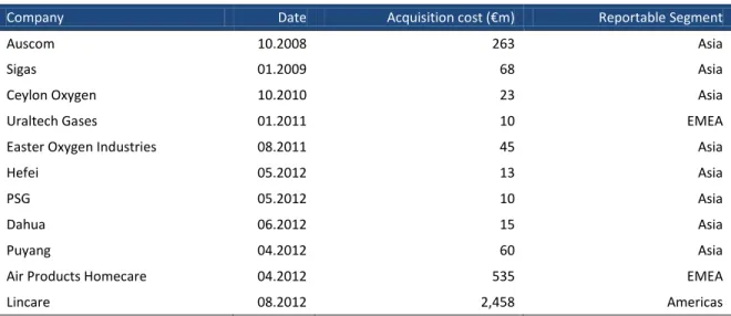
Linde’s business strategy is based on the generation of increasing profits due to a sustainable growth model. This includes the expansion of the international business, the creation of innovative products and services and the increase of the customers’ usage when buying Linde products. Due to this policy, Linde acquired the homecare business (a subdivision of the medical gases segment) of Air Products and the whole business of Lincare in 2012, enabling the company to become the worldwide leader in this segment. Although these acquisitions were the largest within the last years, Linde’s focuses not only on organic growth but also on consolidation as can be observed when looking at the following table:
Table 1: Linde Acquisition Overview 2008 – 2012 by Reportable Segments
Source: The Linde Group, Annual reports, 2008 - 2012
Besides this consolidation strategy Linde drives is business through a constant investment policy, represented by a long-term capital expenditure (“CapEx”) target of 13% compared to total revenue (The Linde Group, Annual report, 2012). Additionally, Linde presents itself with a strong strategic focus on its actual business areas. This strategy led to the sale of
Company Date Acquisition cost (€m) Reportable Segment
Auscom 10.2008 263 Asia
Sigas 01.2009 68 Asia
Ceylon Oxygen 10.2010 23 Asia
Uraltech Gases 01.2011 10 EMEA
Easter Oxygen Industries 08.2011 45 Asia
Hefei 05.2012 13 Asia
PSG 05.2012 10 Asia
Dahua 06.2012 15 Asia
Puyang 04.2012 60 Asia
Air Products Homecare 04.2012 535 EMEA
the company’s historical core business, the refrigeration division, to US based Carrier Corporation in 2004 (Linde AG, 2004).
As previously stated, market trends are expected to drive growth in certain product areas, namely LNG and healthcare, which both represent core areas of Linde’s business. While growth for the first area is mainly driven by changes in the energy market, sales of the latter products will be influenced by structural factors like demographic change and higher living expectations of the population (Ernst & Young, 2011).
Looking at the industrial environment, clean energy in terms of CO2 reduction will increase its importance constantly, leading to an expected global market size of €2 - €3bn in 2020 according to Linde estimations (The Linde Group, Full year results 2012: Determination, 2013). Further, the growing LNG market can also be described as an important driver for Linde’s business, not only for gases but also for the engineering division, as increasing demand for LNG will also drive the division’s activities in terms of building LNG plants and terminals.
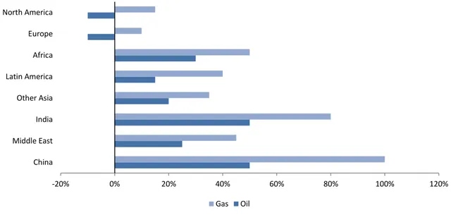
Generally, the shortage of oil and the pricing mechanism will lead to a significant increase in demand for natural gas in the future as can be obtained from the following figure:
Figure 2: Gas and Oil Demand Comparison by Geographies between 2011 and 2025
Source: Avaldsnes, 2013
Taking a glance at the chart, it can be obtained that besides the generally increasing demand for gas, the main growth drivers are the developments in the emerging markets, leading to another strategic focus of Linde:
The company presents significant investments in those markets, with reported revenues of €4.5bn in 2012 (The Linde Group, Business & Governance: Business Opportunities, 2012).
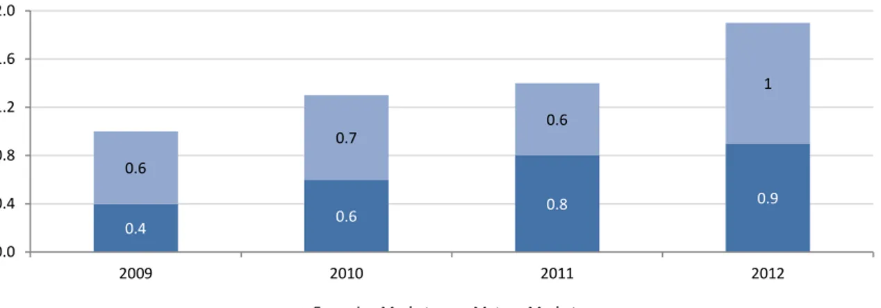
Those results are based on Linde’s constant investment strategy in its emerging market business, being evident when looking at the company’s CapEx composition:
-20% 0% 20% 40% 60% 80% 100% 120% China Middle East India Other Asia Latin America Africa Europe North America Gas Oil
Figure 3: Capital Expenditure in Emerging and Developed Markets in €m
Source: The Linde Group, Full year results 2012: Determination, 2013
As can be obtained, Linde constantly increased its investments in emerging markets and in 2012 almost 50% of its total CapEx was invested in those economies, indicating the strategic importance of these regions for the company’s actual and future activities. As a result, Linde presents itself as the market leader in all major growth markets, including Eastern Europe, Greater China, Southeast Asia and South Africa (The Linde Group, Full year results 2012: Determination, 2013). For other regions, Linde also holds top 3 positions, with the exception of Canada, Spain and Italy where the company doesen’t have significant activities until today. With Compounded Annual Growth Rates (“CAGR”) for industrial and medical gases consumption of 4% (mature markets) and 10% (emerging markets) from 2010 until 2012, Linde can be described as well positioned in those regions. Increased industrialization and wealth is expected to drive those growth grates in the emerging markets also for future periods (The Linde Group, Full year results 2012: Determination, 2013).
Besides organic and external growth, Linde is also focused on increased efficiency. This strategic focus led to the implementation of the High Performance Organization (“HPO”) program, which was initiated in 2009 and which is planned to enable significant cost
0.4 0.6 0.8 0.9 0.6 0.7 0.6 1 0.0 0.4 0.8 1.2 1.6 2.0 2009 2010 2011 2012
savings until 2016. In 2012, Linde reported cost savings of €780m that were achieved through this program and expects further cost saving potentials up to €900m until 2016 (The Linde Group, Annual report, 2012). The main mechanics to enable this decrease in expected costs to be named are:
- Standardization and automation of filling plants
- Product standardization and global roll-out of e-procurement - Optimization of total production and distribution cost
- Shared service centers
The total amount of saving based on those strategies is expected to be divided as follows:
Figure 4: Expected Cost Savings by Segments
Source: The Linde Group, Full year results 2012: Determination, 2013
3.1.4 Stock Information
Linde is a publicly traded company with a stock price of €148.20 (06.03.2014) and a market capitalization of more than €27.2bn (Bloomberg, Bloomberg Markets, 2014). The stocks are mainly held by institutional shareholders (81%) whereas only 19% of the shares are owned by private investors. As can be obtained, shareholders are based all over the world, with the majority being Americans or Germans:
20%
30% 35%
15% Cylinder Supply Chain
Procurement Bulk Supply Chain SG&A
Figure 5: Linde Shareholder Structure by Regions
Source: The Linde Group, Annual report, 2012
Looking at Linde’s historical performance, a clear upwards trend can be observed considering the last five years. After a weaker timeframe within the 2008 financial crisis, the stock recovered constantly since 2009 and reached an all-time high of more than €153 in May 2013 and remains strong until today. In 2012, Linde’s stock closed at €132.00 on December 31st, representing an increase of 14.8% when compared to the previous year. The stocks are traded at all major German stock exchanges and in Zurich. Linde is also listed in the DAX 30.
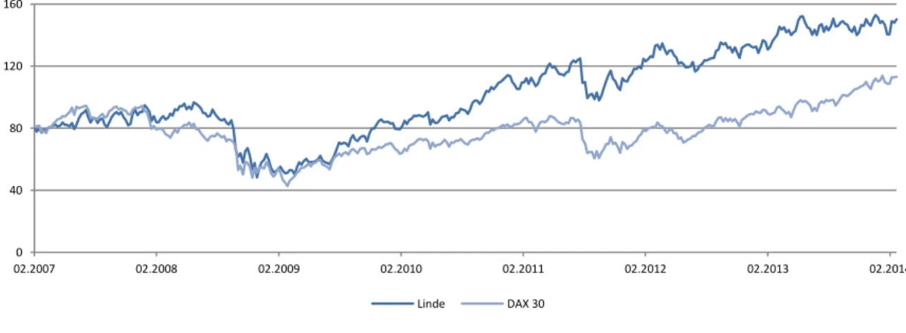
The following figure presents the development of the Linde stock in comparison with the return of the DAX 30 from February 2007 until February 2014:
45% 16% 14% 12% 9% 4% US Germany UK Others France Asia
Figure 6: Linde and DAX 30 Historical Price Developments from 2007 – 2014 in €
Source: Bloomberg
One can observe that the general development of the DAX 30 and the Linde stock is almost identical until February 2009. Afterwards, Linde returns are constantly higher but still the general trend of the chart in terms of increases and decreases remains quite comparable. Consequently, it can be concluded that the Linde stock generally follows the movements of the DAX but with higher returns since 2009.
3.2 The Industrial Gases Industry
Although Linde’s business activities are divided into gas, engineering and others, Linde is mainly part of the industrial gases industry, represented by 80% of Linde total sales being generated within this sector (2012) as previously presented. After the economic crisis in recent years the industry recovered in 2012, enabling Linde a sales growth of 11,1% compared to the previous period. Still this growth is also attributable to Linde’s acquisitions, which will be analyzed in the historical financials development paragraph. Industrial gases are used in all of the major industries and can be divided into several categories, as described previously.
0 40 80 120 160 02.2007 02.2008 02.2009 02.2010 02.2011 02.2012 02.2013 02.2014 Linde DAX 30
The industry can be characterized as stable, whereas the medical gases sector (being part of the industrial gases) can be considered a rapidly growing market due to demographic developments and the increasing demand for healthcare services (Ernst & Young, 2011). Although this sector is of high strategic interest for Linde it only accounts for 20% of the company’s sales in gases division (as of 2012). Consequently, the upcoming forecast will not be specifically focused on the healthcare market, as the general growth potential in this segment is considered in the sales impact of the acquisition of Lincare in 2012. Generally, the industrial gases market is expected to reach $58.4bn in 2018, which equals a CAGR of 6.3% since 2012. Growth drivers to be mentioned, causing this development are the generally increased demand for industrial gases and the economic growth in emerging markets. Challenges are expected in terms of increasing transportation and storage costs, making efficiency increases one of the challenges that have to be faced in the future (Transparency Market Research, 2013).
The market has many competitors, many of them being local companies, but regarding worldwide market shares, four big global players namely Linde, Air Liquide, Praxair and Air Products can be identified (Lecorvasier, 2010). With a market share of 22%, Air Liquide is the largest company worldwide, followed by Linde (Kamp, 2012).
The following table presents an overview of Linde’s main competitors which will also represent the peer group for the upcoming Multiple Valuation:
Table 2: Linde - Main Competitors Key Data
in € million Air Liquide Praxair Air Products
Financials (2012) Revenues 15,326 8,491 7,272 EBIT 2,610 1,844 1,160 EBIT Margin 17.0% 21.7% 16.0% Net Income 1,609 1,280 883 Profit Margin 10.5% 15.1% 12.1% General Information Geographies Americas EMEA Asia/Pacific Products Gases Chemicals Equipment Services Market Information (05.03.2014) Share Price (€) 99.26 95.32 89.14 Shares Outstanding 312.89 293.97 211.67 Market Capitalization 31,057 28,021 18,868 Cash Dividend (€) 2.55 0.47 0,52
Sources: Bloomberg; Air Liquide, 2012; Praxair, 2012; Air Products, 2012
4. Valuation
Before presenting the details of the valuation of Linde, a general note has to be made, as this thesis is delivered on March 10th 2014. Linde will publish its 2013 annual report on March 17th 2014, meaning that historical financial data for the entire 2013 fiscal year were not available. Due to that, the historical numbers analysis will only consider the period from 2008 – 2012, while the forecasted data will include the estimations for 2013. Nevertheless, information provided by the company in the Q3 Interim Report 2013 is considered in this report and is in line with the estimations made for the 2013 fiscal year. However, the 2013 financials will not be considered for the DCF Valuation, as these values
are assumed to be historical for valuation purposes. Nevertheless, for the upcoming transition from enterprise value to equity value, the 2013 data will be considered as the forecast will be made from 2014 – 2018, meaning that the 2013 numbers will be the latest “historical” data available.
The estimation of Linde’s price per share will be based on two different valuation techniques, namely the DCF Valuation and the Multiple Approach, using selected peer group multiples to estimate Linde’s value. Due to a better understanding of the relevant growth drivers within the company, a detailed historical data analysis based on the financial years 2008 – 2012 is presented ahead of the actual forecast of the financials. Additionally, these data will give insights into Linde’s strengths and potential weaknesses and through that allow a more detailed and straight to the point company analysis. After the aforementioned valuations, a sensitivity analysis will provide further insights into selected valuation positions and their impact onto the final result.
4.1 Historical Data Analysis
Understanding Linde’s financial data will be crucial for the valuation process. Due to that, selected balance sheet and income statement items will be presented and analyzed to enable an overview of the company’s business activities. Starting with the balance sheet, the following table provides an overview of Linde’s historical development of its main assets:
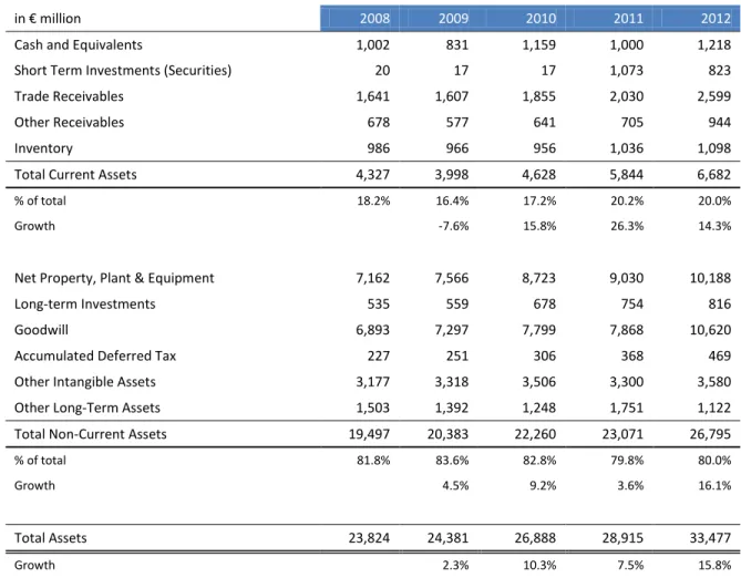
4.1.1 Balance Sheet – Historical Performance Overview Table 3: Balance Sheet 2008 – 2012 (Assets)
in € million 2008 2009 2010 2011 2012
Cash and Equivalents 1,002 831 1,159 1,000 1,218
Short Term Investments (Securities) 20 17 17 1,073 823
Trade Receivables 1,641 1,607 1,855 2,030 2,599
Other Receivables 678 577 641 705 944
Inventory 986 966 956 1,036 1,098
Total Current Assets 4,327 3,998 4,628 5,844 6,682
% of total 18.2% 16.4% 17.2% 20.2% 20.0%
Growth -7.6% 15.8% 26.3% 14.3%
Net Property, Plant & Equipment 7,162 7,566 8,723 9,030 10,188
Long-term Investments 535 559 678 754 816
Goodwill 6,893 7,297 7,799 7,868 10,620
Accumulated Deferred Tax 227 251 306 368 469
Other Intangible Assets 3,177 3,318 3,506 3,300 3,580
Other Long-Term Assets 1,503 1,392 1,248 1,751 1,122
Total Non-Current Assets 19,497 20,383 22,260 23,071 26,795
% of total 81.8% 83.6% 82.8% 79.8% 80.0%
Growth 4.5% 9.2% 3.6% 16.1%
Total Assets 23,824 24,381 26,888 28,915 33,477
Growth 2.3% 10.3% 7.5% 15.8%
Source: The Linde Group, Annual reports, 2008 - 2012
Taking a glance at the 2012 numbers, it can be observed that Linde reports total assets of €33,477m, divided into current and non-current assets, with the latter representing the major asset class with a total share of 80%. Nevertheless, current assets showed slightly lower growth rates within the selected period, resulting in a growth of 14.3% in 2012 for current- and 16.1% for non-current assets. Concerning the entire period considered, total assets showed a continuous growth since 2009 with a slight decrease in 2011 and a low in 2009, caused by the outbreak of the global financial crisis.
Current assets mainly include cash & short term investments, receivables and inventory. While the cash position remains rather constant, short term investments increased significantly from 2010 to 2011. This increase is mainly due to Linde’s investments into available for sale and held to maturity securities totaling €1,073m in 2011. Although this value slightly decreased in 2012 due to the Group financing its acquisitions, short term investments still remain at €823m (Linde annual report, 2012). Regarding receivables, trade receivables represent the major position in Linde’s balance sheet with a value of €2,599m in 2012 and include receivables from percentage of completion contracts (€222m in 2012) and other trade receivables of €2,377m. Inventory mainly includes work in progress goods and finished goods totaling to €1,098m in 2012. It can be concluded that short-term assets showed a constant growth within the last years, mainly based on trade receivables and investments into securities in 2011 and 2012.
Concerning non-current assets, tangible assets, intangible assets and goodwill represent the major positions to be analyzed. Tangible assets include land, land rights and buildings (€1,528m), technical equipment and machinery (€6,843m), fixtures, furniture and equipment (€352m) as well as plants under construction (€1,465), totaling to a net book value of €10,188m in 2012 and representing a growth of 12.8% compared to 2011. The growth in 2012 is mainly due to additions as a result of CapEx in the gases division for on-site projects, rising from €1,439m in 2011 to €1,901m in 2012 and affected technical equipment and machinery. Linde’s intangible assets increased from €3,300m to €3,580m in 2012. As will be presented for goodwill, this is mainly due to the company’s acquisitions that have taken place within the past period. This strategy led to rises in customer relationships and brand names by €344m in the reported timeframe. After a rather small increase in precedent years, goodwill grew significantly in 2012. Main drivers for this development to be named are again the acquisition of Lincare, resulting in an increase in goodwill of €2,605m and the acquisition of Air Products’ Continental European homecare
business. Further, goodwill is based on the acquisition of BOC group in 2006 (€4,843m) and €3,064m for other previous acquisitions.
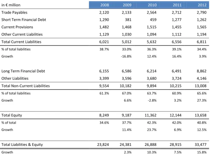
Table 4: Balance Sheet 2008 – 2012 (Liabilities)
Source: The Linde Group, Annual reports, 2008 - 2012
In terms of liabilities, Linde reported current liabilities of €6,811m and non-current liabilities of €13,008m in 2012, where the first represents 34.4% and the latter 65.6% of the group’s total debt. Current debt comprises mainly accounts payable (€2,790m in 2012) and other current provisions of €1,565m. In terms of non-current liabilities, long-term debt arises mainly from subordinated and other bonds due in more than 1 year, which can be observed as largest position within that area. Regarding equity, the company presents a stable growth position since 2008 with a low in 2011. While common stock remained
in € million 2008 2009 2010 2011 2012
Trade Payables 2,120 2,133 2,564 2,712 2,790
Short Term Financial Debt 1,290 381 459 1,277 1,262
Current Provisions 1,482 1,468 1,515 1,455 1,565
Other Current Liabilities 1,129 1,030 1,094 1,112 1,194
Total Current Liabilities 6,021 5,012 5,632 6,556 6,811
% of total liabilities 38.7% 33.0% 36.3% 39.1% 34.4%
Growth -16.8% 12.4% 16.4% 3.9%
Long Term Financial Debt 6,155 6,586 6,214 6,491 8,862
Other Liabilities 3,399 3,596 3,680 3,724 4,146
Total Non-Current Liabilities 9,554 10,182 9,894 10,215 13,008
% of total liabilities 61.3% 67.0% 63.7% 60.9% 65.6%
Growth 6.6% -2.8% 3.2% 27.3%
Total Equity 8,249 9,187 11,362 12,144 13,658
% of total 34.6% 37.7% 42.3% 42.0% 40.8%
Growth 11.4% 23.7% 6.9% 12.5%
Total Liabilities & Equity 23,824 24,381 26,888 28,915 33,477