A PLANNING MODEL FOR OFFSHORE NATURAL GAS TRANSMISSION
Edson K. Iamashita PETROBRAS S.A.
Programa de Doutorado em Engenharia de Reservatório e de Exploração
Universidade Estadual do Norte Fluminense (UENF) Macaé – RJ
Frederico Galaxe José Arica *
Laboratório de Engenharia de Produção
Universidade Estadual do Norte Fluminense (UENF) Campos dos Goytacazes – RJ
[email protected] , [email protected]
* Corresponding author / autor para quem as correspondências devem ser encaminhadas
Recebido em 06/2006; aceito em 12/2007 após 1 revisão Received June 2006; accepted December 2007 after one revision
Abstract
This paper aims at new approach to solve complex integrated offshore gas planning problems, defining the best transmission strategy for a system with a large number of platforms interconnected between them and with delivery points through a complex gas pipeline network (which can be cycled). The problem is formulated as a large quadratic mixed-integer problem, where non-convexity and non-differentiability is found. Because the complexity of the problem, it is proposed a heuristic, in the context of genetic technique, for solving it. Several numerical experiments are presented at the end of this work. The results show that the performance of our approach is very good, being its results very close to exact solutions. The algorithm could be used for sizing and optimization designs of gas pipeline networks, as well as for the gas transmission planning of an existing network, seeking for profit maximization.
Keywords: natural gas; transmission networks; genetic meta-heuristic.
Resumo
Este trabalho visa apresentar uma nova abordagem para resolver o problema de planejamento integrado de movimentação de gás natural offshore, definindo a melhor estratégia de transmissão para um sistema com um grande número de plataformas interconectadas com pontos de distribuição por meio de uma rede complexa de gasodutos (a qual pode possuir ciclos). O problema formula-se como um modelo misto-inteiro quadrático de grande porte, não convexo e não diferenciável. Devido à complexidade do problema, propõe-se uma heurística com abordagem genética para resolvê-lo. Vários experimentos numéricos se apresentam ao final deste trabalho. Os resultados mostram que o desempenho de nossa abordagem é muito boa, obtendo soluções muito próximas de soluções exatas. O algoritmo genético proposto poderá ser usado para dimensionar e otimizar o planejamento de redes complexas de gasodutos, tanto como para planejamento da transmissão de gás num gasoduto existente, procurando maximizar lucros.
1. Introduction
The planning of balance and utilization of associated natural gas to the oil produced by platforms having a transmission system integrated by regular gas pipelines is complex, involving a large number of operational variables and constraints such as: compressors shut-downs, gas pipelines and equipment limitations, need of gas lift, gas demand, volumetric balance, etc. Such variables and constraints can generate several options to the gas destinations of each platform: available gas for sale, injected gas or produced from storage reservoirs, injected gas for secondary recovery, injected gas for gas lift, gas consumed at platform, gas transferred between platforms and flared gas.
The optimization of gas balance also takes into account, in addition to the volumetric balance under standard conditions, such economic parameters as: oil and natural gas prices, costs in compression, treatment, transport, gas injection, etc.
When gas flows through a gas pipeline network it occurs a loss of energy and pressure drop due to both friction between gas and the pipe inner wall and the heat transfer existing between the gas and the environment. To make possible the transportation of gas from platforms to distribution and consumption centers it must be compressed to high pressures. The issue at hand is to determine the best configuration of compressors (at platforms) and gas pipelines operation (transported flows and generated pressures) aiming to compress and transport the produced gas with the highest profit possible. General assumption of steady-state system and isothermal process (constant ambient temperature) are made.
From the optimization viewpoint the mathematical structure that defines such problem is a large scale non-convex mixed-integer quadratic model, which, as observed by Raman & Grossmann (1991), is NP-complete, with exception of particular structures. A direct implication of this complexity is that in the worse case the solution time employed by any exact algorithm grows exponentially with the problem size.
A version, in some way, more general than this problem, consisting of the natural gas transmission problem considering intermediary compressors stations to raise the pressure that decreases during flowing through the network, can be found in Rios-Mercado et al. (2000, 2004) and Wolf (2003). Nevertheless, our algorithmic approach is quite different than that. On the other hand, the problem treated here has particularities that modify the more general version model. Because of characteristics of the offshore associated gas production system the planning of gas uses must be considered at each source node (offshore production platforms) for several processing purposes (see Iamashita et al., 2005). Additionally, different from the general version, the objective function of the model here introduced is non-differentiable.
2. The problem definition and steady-state model description
diminish the pressure gradient in the well vertical section and stimulate the production), is separated from the oil and water through production separators. When leaving the production separators, the oil and remaining gas solution is directed to the surge tank. There, the gas remaining in oil is separated near sea level pressure.
The gas from the surge tank is compressed through a platform compressor station (composed by several compressors) together with the gas from the production separators. Compressors are equipments in charge of pressure increase so that the gas can be used for consumption, gas lift injection, secondary recovery injection and storage or transferred for sale through gas pipelines. The operational compressors in the period may consume high-pressure gas or diesel to carry out the work of gas pressure increase (some compressors can also be activated by electric motors). On the other hand, there may be interconnection at low and medium pressure between two or more platforms so that the excess of gas in a certain platform may be compressed in a different platform with available compression capacity.
The causes leading to gas flaring at platforms are several: production system instability (mainly when it is caused by severe well gushes), instrumentation and automation problems (electric power failures, incorrect alarms, etc.), gas compressors capacity constraints, gas pipelines constraints, and gas demand constraint (for example, demand below the system total gas offer). The remaining natural gas in platforms (i.e., the gas after storage, consumption, injection and flaring) outflows through the gas pipeline network up to the final distribution and sale point. Some pipelines can have two ways; i.e., in some periods, they can have gas flow in one direction and in other periods can have the opposite direction flow depending on the load distribution in the system.
This way, before the gas be injected in the pipeline network, the different demands in the platforms can be described considering that there exists equipments that will regulate the outlet flows (modeling by the variables si of each platform – source node i), such as: compressors, electrical generators, burners, etc. Thus, for each platform i the following volume balance relationship can be defined:
1
( * ), platform, cAi
ij ij j
i i i i i
s comp glc inj cstg KccA xcA i
=
= − − − −∑ ∀ (1)
where:
glci : gas lift volume injected in the oil production column (non-negative); inji : gas volume injected in storage wells or secondary recovery (non-negative); cstgi : electric power generators gas consumption(non-negative);
compi : compressed gas volume (non-negative); cAi : number of compressors at platform;
KccAi,j : constants defining the compressor consumption j at platform;
xcAi,j : decision variables 0-1 indicating the compressor j operation (turned on or turned off). Naturally, some additional relations among the above variables and other ones must be satisfied to describe completely the gas balance of platform demands. The following relations establish the volumetric balance constraints under standard conditions considered for each platform i:
0≤inji≤injmaxi, (2)
0≤dispcompi=KgAi+Kgli+recebibp−transfibp−queii, (3)
where the variable dispcomp defines the low pressure available gas for compression in each platform; i.e., the reservoir gas associated to the oil (KgA, constant for each platform), plus gas lift returned after lifted the oil (Kgl, constant for each platform), plus gas received from another platform (receb, non-negative variable), subtracted the low pressure gas transferred to another platform (transf, non-negative variable) and the flared gas (quei, non-negative variable);
i i i i
comp +quei −glc =KgA, (4)
which establishes that in each platform the gas that is not compressed will be flared;
1
0 cAi
i ij ij
j
comp KcA xcA
=
−
∑
≤ , (5)0
i i
comp −discomp ≤ , (6)
0 i
comp ≥ , (7)
these relations guarantee that the platform i will compress the lower positive value between the compressors capacity (KcAij: j compressor capacity at platform i) and the available gas for compression;
i i P
s demand ∈
≤
∑
, (8)which determines the constraint that control the maximum gas volume that could send to costumers (P is the index set of platforms);
0≤glci≤Kgli, (9)
establishes that gas lift will be between 0 and the proposed gas lift volume (Kgl) (it is necessary to introduce this constraint because in some compression configurations of platform i the compression capacity is lower than the proposed gas lift volume Kgli);
0≤queii≤KgAi, (10)
which limits the gas flare (quei) to the produced gas volume.
Once the gas consumption demands are satisfied in each platform i, a volume si of gas (defined by the above relations) is injected in the pipeline network. Thus, some constraints associated to the gas flows circulating in gas pipeline sections and pressures at the ends of each section must be considered.
To do this, let’s see that the gas pipeline network can be represented by a directed graph (c.f., Rios-Mercado et al., 2004; Wolf, 2003). Consider a network with n nodes and l pipes. Such network can be described by an oriented (directed) graph G=( , )N D , where
Thus, under steady-state networks conditions assumed, a first relationship, called flow balance, for each node k∈N is:
( , ) ( , )
,
ki ik k
k i D i k D
f f s
∈ ∈
= +
∑
∑
(11)where sk ≥0 if the k node is a supply node (given by relation (1)), sk <0 if the k node is a delivery node (eventually, given by relation (1)) and sk =0 in another case. The s vector, called source vector, should also attend the relationship k 0.
i N
s
∈
=
∑
Another relationship to consider (under the assumed conditions), called pressure-flow equation, between the flow fij, circulating within the gas pipeline section ( , )i j ∈D and the pressures pi and pj at the ends of the pipe, describing the dynamic of the flow in the pipe, is:
2 2
i j ij ij ij
p −p =c f f , (12)
where the constant cij>0 is the pipe resistance coefficient, that depends on the pipeline physical attributes. Note that the sign of the right hand of relation (12) can be positive or negative (depending on the sign of fij), meaning that pi is greater than pj or vice versa, respectively. In the problem hereby addressed, there is only one known flow delivering node (the demand node), let’s say node n, where the pressure is fixed, i.e., pn=pn. The other node pressures should satisfy box constraints:
0≤ piL≤ pi≤piU,i∈N\ { }n , (13)
where pL and pU are given vectors.
Relations (11) and (12), above, can be stated in a short form by using some additional concepts associated to the graph G. Considering the network with n nodes and l pipes, the node-pipe incidence matrixA of graph G is a matrix of dimension n l× whose elements are given by:
1, if arc exits node ; 1, if arc enters node ; 0, in other cases. ij
j i
a j i
= −
(14)
Being pi the pressure in node i and pT =
(
p1,…,pn)
, consider the source vector s, as in (11). Recall also that the source vector should satisfy the relationship:0. i i N
s
∈
=
∑
(15)Thus, the gas pipeline network flows and pressures balance ((11)-12)) can be written as:
2 ,
( ), T
Af s A p b f
=
where the indexes were redefined, so that fT =
(
f1,…,fl)
is the flow vector (with fj being the flow in pipeline j∈ …{
1, ,l}
and l= D ), (p2)T =(
p12,…,pn2)
and bj( )f =c fj j fj , where cj is the given positive resistance coefficient of pipe j∈ …{
1, ,l}
. As long as the rank of A is (n−1), considering the reduced matrix AR as matrix A without the last row and vector sR as vector s without the last component, we have that the system Af =s, in (16), is equivalent to the system A fR =sR. Consequently instead of considering the system (16) as the pressure and flow balance, taking in account (13), it is used the following system:2 ,
( ).
0 , 1, , 1, .
R R
T
L U
i i i n n
A f s
A p b f
p p p i n p p
= =
≤ ≤ ≤ ∀ = … − =
(17)
Thus, the balance system, (11)-(13), can be expressed by the relationship (17).
Note that the set of feasible solutions for pressure balance equations, because the second equation in (17), is non-convex, which increases the difficulty to solve the problem.
On the other hand, the objective function associated to the problem of natural gas transmission planning here considered is the profit function, which considers the next revenues and costs:
• Gas sale revenue, formed by the sum of gas volumes available for sale in each platform multiplied by the sale prices thereof (Ps).
• Gas Lift revenue, formed by the sum of the wells additional oil volumes produced according to gas lift multiplied by the relevant oil sale prices (Pglc), corresponding to the gas lift injection financial gain. (As there may be limitations in the compression system the required volume of gas lift may not be met due to an unfavorable economic analysis for the company. In such case the system should calculate the volume of optimized gas lift).
• Unit revenue from the injection for secondary recovery (Prec), corresponding to the amounts of additional oil volumes recovered in function of the gas injection and their prices.
• Unit revenue from injected gas for storage, formed by the relevant amounts of unburned gas (Pinj).
• Take or Pay cost (DifT or p), unit fine per delivery of volume below the minimum amount agreed upon (demand d).
In this work, it is used the following objective function:
(
, , ,)
T or pT T T T T
s glc inj rec rec quei
F s f x y =P s+P glc+P inj+P inj −P quei−Dif fine, (18)
where yT =(glcT,injT,injTrec,compT,cstgT,recebT,queiT,transfT,cstcT) is the platforms operational variables vector. Note that function F( )⋅ is non-differentiable.
Thus, the problem of determining the configuration of compressors in the platforms (binary vector x), the operation of platforms (vector y and vector s), the flow vector (f ) and the pressure vector (p) to maximize the profit function is given by:
(
)
maximize F s f x y, , ,
Subject to:
Balance system (17) and relations (1)-(10).
Using the before introduced notation, the problem takes the form:
{ }
2maximize ( , , , )
( )
, 1, , 1
, 0 , 0 , , 0,1 ,
T
P
U U
i i i
m S
n n i
i P
F f s y x
Af s
A p b f
Cy Dx s
Ey e
p p p i n
p p f y y s d x
∈
= =
+ =
≤
≤ ≤ = −
= ≤ ≤ ≤
∑
≤ ∈…
(19)
where vector f is the flow vector circulating in the network; vector s is the source vector; vector y is the vector of operational variables in the platforms; matrix A is the node-pipe incidence matrix of the graph G; vector p is the pressure vector; bj( )f =c fj j fj and cj is the given positive pipe resistance coefficient; matrices C, D and E are adequate matrices (given by relations (3)-(6)); vector x is the binary vector associated to compressors operation; P is the index set of platforms; vector sP is the source vector associated to platforms; e is a given constant vector; vectors pL and pU are, respectively, lower and upper limits for pressure vector; n is the number of nodes in the network; vector yS is an upper bounded associated to operational variables in the platforms; d is the given demand of the natural gas; and, m is the total number of compressors in the system.
3. The proposed heuristic
The second procedure begins once the source vector components corresponding to platforms are defined. At this stage, we try to drop those flows through the gas pipeline network. Thus a vector of flows f and a vector of pressures p satisfying relation (16) must be found. If these vectors are not feasible (because of the pressure box constraints, (13)), it means that the source vectors components at platforms must be diminished. Then they are decreased, adequately (increasing inj first and then quei), and return to the first procedure, until be found components si, for i∈P, a vector of flows f and a vector of pressures p satisfying relation (17). In this way, it is associated a feasible solution to each configuration of compressors, for a given vector s (defined by (1)). A master iteration of the heuristic is completed changing, heuristically, the compressors configuration if an end condition is not attained. This paper presents an algorithm that implements the above heuristic using genetic techniques.
More formally, we establish the following considerations. It is said that platform i has a certain compression configuration when a certain set of values 0-1 is considered for the binary variables xcAij (compressor j operation state at platform i). Therefore the all possible compression configurations of the set of platforms are formed by sets of arrangements of 0’s and 1’s (with the arrangement size corresponding to the total number of network compressors). Considering these possible configurations in the genetic algorithmic proposal presented herein, each possible arrangement is a chromosome and each 0 or 1 of the chromosome is called a gene, representing a state of operation (turned on or turned off) of the corresponding compressor in the respective platform.
The proposed algorithm operates according to the next strategy: given the offshore gas pipeline network, a certain operation configuration of existing compressors and a certain level of gas flaring in each platform, the feasibility of gas transmission (i.e., the transmission of flows si from each platform i) is determined by the balance system solution (16) (determination of flow variables f for the gas pipeline section and pressure p in the respective nodes). If the vector p does not satisfy (13), s is considered non-feasible and, by maintaining the configuration and all the uses of gas in the platforms, the storage gas injection and flaring gas is conveniently increased going again to the balance method solution until reaching the gas transmission feasibility.
The following result is known:
Theorem 1 (Theorem 1, Rios-Mercado et al., 2000). Let be G a graph with n nodes and l arcs and T a spanning tree of graph G′. Then,
(a) The number of edges in the spanning tree T is n-1 and the number of chords corresponding to the spanning tree T is l-n+1.
(b) The number of fundamental cycles corresponding to the spanning tree T is l-n+1. Every other cycle in G′ is a linear combination of fundamental cycles.
On the other hand, each cycle in G, after arbitrarily associating a direction thereto (clockwise or counterclockwise), can be seen as a “directed” cycle and represented by a vector of components 1, -1 or 0 according to the direction of each arc in G in relation to the cycle. This can be represented by the cycle matrix B, where each row corresponds to a cycle vector and each column to an arc, defined by
1, if cycle contains arc and directions coincide; 1, if cycle contains arc and directions do not coincide; 0, if cycle does not contain arc . ij
i j
b i j
i j
= −
(20)
According to Theorem 1, only l− +n 1 fundamental cycle vectors related to one spanning tree are independent. Once cycle matrix comprising these fundamental cycle vectors l− +n 1 is called reduced cycle matrix, it is denoted by BR and has dimension
(
l− + ×n 1)
l.Matrices AR and BR are related by the following proposition:
Theorem 2 (Theorem 2, Rios-Mercado et al., 2000). Let be G a graph, with AR and BR its incidence and reduced cycle matrixes, respectively. Then,
0
T T
R R R R
A B =B A = .
Thus, from the relationship (17) and from Theorem 2, considering p= p2, the flow and pressure balance system can be written as:
, ( ) 0,
( ).
R R
R T
A f s
B b f
A p b f
= = =
(21)
The advantage of system (21), in relation to (17), is that the first two equation sets (A fR =sR e B b fR ( )=0) have unique solution (Corollary 2, Rios-Mercado et al., 2000). So that, once the solution f of these equations is found, the vector b f( ) can be calculated and then the solution p of equation A pT =b f( ) found, thus determining a solution for the balance system (21). The described sets of equations are solved, in our algorithm, by the Newton-Raphson method, which, considering the characteristics of system (21), is very well-behaved.
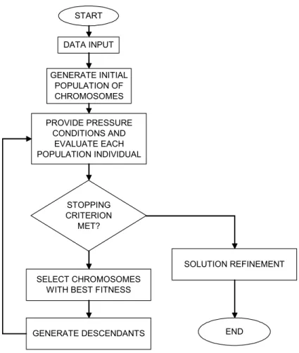
Step 1. (Parameter Input) Production of gas, gas lift, data from compressors and gas pipelines, delivery pressure, network matrix incidence (AR), reduced cycle matrix BR, scheduled outages, etc. Set the iteration counter t=1.
Step 2. (Generation of Initial Population of Individuals – chromosomes) Generate the population P t( ) that will represent a set of possible solutions for the compressors operational configuration (the initial population is randomly generated or is defined from a pre-established criterion, forming the chromosome with genes 0-1). Each gene will represent the operation decision variables of the compressors (xcAij). The population size used in the tests was 40 chromosomes.
Step 3. (Feasibility of the Current Population) First, for each chromosome, this step provides a feasible vector s, a feasible flow vector f and a feasible pressure vector p; then, it assesses this feasible population:
- For each chromosome, calculate, for each platform i, the components si
(of source vector s) using relation (1), considering relations (2)-(10).
- Solve the flow and pressure balance system (21) (using the Newton-Raphson method).
- Check if pressure conditions are satisfied for each platform, i.e., if relation (13) is satisfied.
If such conditions are not satisfied:
• Increase the gas injection for storage, with the step of 10% of the produced gas, until the pressure conditions are attended or until the maximum injection limit is reached.
• Increase the gas burning in platforms, with the step of 10% of the produced gas in the platform that has the higher pressure up the operational limited pressure, until the pressure conditions are attended.
Re-calculate the values of si (lower than the initial values) and calculate the value of the objective function F (Fitness function).
Step 4. (Stop Condition)While stop condition is not met (here we use t<K, where K is the parameter number of generations):
• Generate a new population P t( +1) from P t( ) (current population). For the selection of chromosomes that will generate descendants, the best individuals of the population divided into subgroups are chosen. The crossover and mutation operators are used in this stage (we used the crossover probability of 70% and mutation probability of the 0,5%). Set t= +t 1.
• Return to Step 3.
Remark: In the realized tests, using various pipeline networks, we conclude that the solution was stabilized between the 20 and 30 generations. Thus, here, it was used K=30.
START
DATA INPUT
GENERATE INITIAL POPULATION OF CHROMOSOMES
PROVIDE PRESSURE CONDITIONS AND
EVALUATE EACH POPULATION INDIVIDUAL
STOPPING CRITERION
MET?
SELECT CHROMOSOMES WITH BEST FITNESS
GENERATE DESCENDANTS
SOLUTION REFINEMENT
END
Figure 1 – Genetic Algorithm Flowchart.
4. Results
The algorithm proposed here, codified in C++, was tested in several problems of different size, with promising results. It can be used for planning and sizing due to the results precision, mainly for the calculation of flow and pressure drop in the pipeline network. The model considers pipeline networks which may contain several cycles.
A total of 31 different problems were tested. The purpose of deal with some small size problem was to compare the performance of our genetic algorithm with the exact solutions (using LINGO software). The main parameters of the problems are the number of nodes and arcs of the network, the existence and number of cycles, the number of source nodes (platforms) and number and kind of compressors considered.
It is important to mention that we use LINGO software only to compare the quality of results, concerning the approximation of exact and heuristic results. Naturally, LINGO (or any other usual library software) can not be used in a straight way in the model, because the non-differentiability of the objective function and the pressure-flow equations (12). Thus, to let the use of LINGO, once obtained the heuristic results, the incidence matrices were adequately changed (reoriented) to eliminate the non-differentiability in equation (12). On the other hand, in all tests, the demand d in the model was set sufficiently low as to turn the objective function differentiable. Naturally, those changes do not change the heuristics results, but make possible to use any usual library software.
The problems tested have de following characteristics:
1. Network 01: There were considered the next cycle pipelines a. 20 nodes, 26 arcs, 10 platforms and 7 cycles. b. 21 nodes, 27 arcs, 11 platforms and 7 cycles. c. 22 nodes, 28 arcs, 12 platforms and 7 cycles. d. 23 nodes, 29 arcs, 13 platforms and 7 cycles.
For each network, there were tested cases with 1, 2 and 3 compressors for each platform.
2. Network 02: There were considered the next acyclic pipelines (trees) a. 20 nodes, 19 arcs, 10 platforms.
b. 21 nodes, 20 arcs, 11 platforms. c. 22 nodes, 21 arcs, 12 platforms. d. 23 nodes, 22 arcs, 13 platforms.
For each network, there were tested cases with 1, 2 and 3 compressors for each platform.
3. Network 03: There were considered the next cycle pipelines a. 22 nodes, 29 arcs, 10 platforms and 8 cycles. b. 23 nodes, 30 arcs, 11 platforms and 8 cycles. c. 24 nodes, 31 arcs, 12 platforms and 8 cycles.
For each network, there were tested cases with 1, 2 and 3 compressors for each platform.
4. Network 04: There were considered the next pipelines
5. Network 05: There were considered the next pipelines
a. 70 nodes, 69 arcs, 45 platforms, 118 compressors and without cycles. b. 70 nodes, 74 arcs, 45 platforms, 118 compressors and 5 cycles. c. 70 nodes, 79 arcs, 45 platforms, 118 compressors and 10 cycles. d. 70 nodes, 84 arcs, 45 platforms, 118 compressors and 15 cycles. e. 70 nodes, 89 arcs, 45 platforms, 118 compressors and 20 cycles.
6. Network 06: There were considered the next pipelines
a. 80 nodes, 79 arcs, 49 platforms, 137 compressors and without cycles. b. 80 nodes, 84 arcs, 49 platforms, 137 compressors and 5 cycles. c. 80 nodes, 89 arcs, 49 platforms, 137 compressors and 10 cycles. d. 80 nodes, 94 arcs, 49 platforms, 137 compressors and 15 cycles. e. 80 nodes, 99 arcs, 49 platforms, 137 compressors and 20 cycles.
7. Network 07: There were considered the next pipelines
a. 100 nodes, 99 arcs, 64 platforms, 177 compressors and without cycles. b. 100 nodes, 104 arcs, 64 platforms, 177 compressors and 5 cycles. c. 100 nodes, 109 arcs, 64 platforms, 177 compressors and 10 cycles. d. 100 nodes, 114 arcs, 64 platforms, 177 compressors and 15 cycles. e. 100 nodes, 118 arcs, 64 platforms, 177 compressors and 20 cycles.
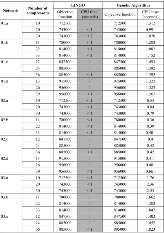
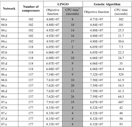
The following two tables present the results of the test problems. Table 1 gives the results relative to small size problems (Network 01 to Network 03) and Table 2 the results relative to medium and large size problems (Network 04 to Network 07).
For small size problems, once known the genetic results, in all the cases was possible to redirect the respective graph to obtain an exact solution to compare with the heuristic one. It was not the purpose to compare times, so the column corresponding to LINGO time, at Table 1 and Table 2, is only referential. The optima objective function coincides in all the cases.
Table 1 – Small size tests results.
LINGO Genetic Algorithm Network Number of
compressors Objective function
CPU time*
(seconds) Objective function
CPU time (seconds)
10 712500 1 712500 1.312
20 743000 < 1 743000 0.991 01.a
30 743000 < 2 743000 1.070 11 780000 < 1 780000 1.282 22 814000 < 1 814000 1.082 01.b
33 814000 < 1 814000 1.152
12 847500 1 847500 1.493
24 885000 1 885000 1.392
01.c
36 885000 < 1 885000 1.392
13 915000 1 915000 1.322
26 956000 1 956000 1.322
01.d
39 956000 < 1 956000 1.262 10 712500 < 1 712500 0.55 20 743000 < 1 743000 0.84 02.a
30 743000 < 1 743000 0.79 11 780000 < 1 780000 0.36 22 814000 < 1 814000 0.39 02.b
33 814000 < 1 814000 0.401
12 847500 1 847500 0.4
24 885000 1 885000 0.42
02.c
36 885000 < 1 885000 0.42
13 915000 1 915000 0.411
26 956000 1 956000 0.401
02.d
39 956000 < 1 956000 0.661 10 712500 < 1 712500 1.76 20 743000 < 1 743000 2.36 03.a
30 743000 < 1 743000 2.53
11 780000 1 780000 1.662
22 814000 1 814000 1.382
03.b
33 814000 1 814000 1.842
12 847500 1 847500 1.402
24 885000 1 885000 1.452
03.c
36 885000 < 1 885000 1.823
Table 2 – Medium and large size tests results.
LINGO Genetic Algorithm Network Number of
compressors Objective function
CPU time*
(seconds) Objective function
CPU time (seconds)
04.a 102 4.68E+07 8 4.71E+07 302
04.b 102 4.88E+07 10 4.84E+07 101
04.c 102 4.92E+07 14 4.88E+07 25.5
04.d 102 4.92E+07 16 4.88E+07 21.7
04.e 102 4.93E+07 17 4.88E+07 30.6
05.a 118 6.05E+07 2 6.05E+07 7.5
05.b 118 6.06E+07 8 6.05E+07 22.3
05.c 118 6.08E+07 10 6.06E+07 24.7
05.d 118 6.07E+07 9 6.06E+07 35
05.e 118 6.04E+07 2 6.06E+07 44.4
06.a 137 7.34E+07 9 7.32E+07 529
06.b 137 7.61E+07 10 7.58E+07 61.9
06.c 137 7.62E+07 20 7.59E+07 34.5
06.d 137 7.62E+07 13 7.59E+07 41.3
06.e 137 7.62E+07 26 7.59E+07 64.5
07.a 177 7.91E+07 19 8,07E+07 607
07.b 177 8.33E+07 4 8.32E+07 42
07.c 177 8.33E+07 4 8.32E+07 48
07.d 177 8.33E+07 4 8.32E+07 50
07.e 177 8.33E+07 4 8.32E+07 93
* Recall that this time would have been impossible to obtain without knowing the genetic results.
5. Conclusions
Acknowledgments
The authors would like to thank Alex Alves Gomes and Juliana Tavares Bessa, who help us with an important part of numerical tests, and the referees for their clever remarks. This research has been supported by The (Brazilian) National Council for Scientific and Technological Development (CNPq) and The Research Foundation of Rio de Janeiro State (FAPERJ).
References
(1) Iamashita, E.K; Galaxe, F.; Arica, J.; Iachan, R. & Justiniano, L.R.S. (2005). Um Algoritmo Genético Híbrido para o Planejamento de Movimentação de Gás da Bacia de Campos. XXXVII Simpósio Brasileiro de Pesquisa Operacional. Hotel Serra Azul, Gramado – RS, Brasil.
(2) Raman, R. & Grossmann, I.E. (1991).Relation between MILP Modelling and Logical Inference for Chemical Process Synthesis. Computers and Chemical Engineering, 15(2), 73-84.
(3) Rios-Mercado, R.Z.; Wu, S.; Scott, R.L. & Boyd, E.A. (2000). Preprocessing on Natural Gas Transmission Networks. Technical Report PISIS-2000-01, Graduate Program in Systems Engineering, UANL, San Nicolás de los Garza, México.
(4) Rios-Mercado, R.Z.; Kim, S. & Boyd, E.A. (2004). Efficient Operation of Natural Gas Transmission Systems: A Network-Based Heuristic for Cyclic Structures. Universidad Autónoma de Nuevo León, AP 111 – F, Cd. Universitaria, San Nicolás de los Garza, NL 66450, México ([email protected]).