RANKING GRAPH EDGES BY THE WEIGHT OF THEIR SPANNING ARBORESCENCES OR TREES
Paulo Oswaldo Boaventura-Netto
Program of Production Engineering / COPPE Federal University of Rio de Janeiro (UFRJ) Rio de Janeiro – RJ, Brazil
* Corresponding author / autor para quem as correspondências devem ser encaminhadas
Recebido em 07/2006; aceito em 11/2007 Received July 2006; accepted November 2007
Abstract
A result based on a classic theorem of graph theory is generalized for edge-valued graphs, allowing determination of the total value of the spanning arborescences with a given root and containing a given arc in a directed valued graph. A corresponding result for undirected valued graphs is also presented. In both cases, the technique allows for a ranking of the graph edges by importance under this criterion. This ranking is proposed as a tool to determine the relative importance of the edges of a graph in network vulnerability studies. Some examples of application are presented.
Keywords: graphs; matrix-tree theorem; vulnerability.
Resumo
Um resultado baseado em um teorema clássico da teoria dos grafos é aqui generalizado para grafos valorados, permitindo a determinação do valor total das arborescências parciais com raiz dada que contenham um arco dado, em um grafo orientado valorado. Um resultado correspondente para grafos não orientados valorados é também apresentado. Em ambos os casos, a técnica descrita permite uma hierarquização por importância das ligações do grafo, sob este critério. Esta hierarquização é proposta como uma ferramenta para determinar a importância relativa das ligações de um grafo em estudos sobre vulnerabilidade de redes. Alguns exemplos aplicados são apresentados.
1. Introduction
The study of maximal acyclic structures in directed and undirected graphs, especially those with spanning arborescences and trees, is a classical subject of graph theory, which we follow in this work in order to propose a theoretical tool for network vulnerability analysis. The basic notions and results of graph theory used in the theoretical developments can be found in Harary (1971), Berge (1973), Bondy & Murty (1976) and Gross & Yellen (2005). We will use the notation and concepts as in Berge.
Since the publication by Tutte of the celebrated matrix-tree theorem (see for instance [Be73] ), the theoretical interest of the theme, especially in its relationship with algebraic graph theory, brought to the literature a number of important works such as those of Kelmans (1997), who early in 1965 had already published in the field.
More recently, the interest contributed by applications such as communication networks and structural design has inspired a number of studies dedicated to the building of these structures, subject to various constraints such as total length of shortest paths, Wu et al. (2000), radius bounding, Serdjukov (2001), leaf degree, Kaneko (2001) and minimum diameter, Hassin & Tamir (1995). The structures of fullerene graphs, of interest in organic chemistry, discussed by Brown et al. (1996), also enhanced the interest in research on spanning trees.
The formulation of algorithms for finding graph parameters related to spanning trees and arborescences resulted in works concerning the problem of the k most vital edges, Liang (2001), the unranking of arborescences, Colburn et al. (1996), the counting of minimum-weight spanning trees, Broder & Mayr (1997) and the reliability improvement of a network through a single edge addition, Fard & Lee (2001). A work on digraphs and graphs concerning the effect of link addition and removal on the number of spanning arborescences and trees is found in Boaventura-Netto (1984). Some questions concerning edge-weighted graphs, where the arborescence weight is the product of the weights of its arcs, were first presented by Bott & Mayberry (1954) and more recently discussed by Chung & Langlands (1996).
This work proposes a criterion for ranking the edges of a directed (undirected) graph based on the value of the spanning arborescences (trees) to which it belongs. To that end, we develop a technique using the approach of Boaventura-Netto (1984) and Colburn et al. (1996) to deal with edge-weighted graphs where the substructure weight is given by the sum of edge values.
It is fitting to observe that the total weight of the spanning arborescences (trees) of a graph, calculated for each one as the sum of its edges, could be obtained as shown in Chung & Langlands (1996), substituting exponentials ew(i,j) for the link weights w(i,j) and taking logarithms at the end. While this calculation is theoretically very simple, it would easily cause overflow problems, unless both graph order and edge values were very small. On the other hand, the technique described in Boaventura-Netto (1984) and Colburn et al. (1996) is limited to equal values for every edge.
2. Some theoretical background
Def. 2.1: The Laplacian Q(G) = [qij]of a directed graph G = (X,U) is the matrix given by
qij = d-(j) i = j qij = -aij i ≠ j,
where A(G) = [aij] is the adjacency matrix of G and d-(j) is the indegree of vertex j.
With undirected graphs, we substitute the degree d(j) for the indegree d-(j).
Def. 2.2: The rth-vertex reduced Laplacian of G, Qr(G), is the matrix obtained from Q(G) by the removal of its rth line and column.
Theorem 2.1 (Matrix-tree theorem): Given a directed (undirected) graph G and its Laplacian Q(G), the cardinality of the set Hr(G) of r-SPA (of SPT) is the value of the
determinant of Qr(G) for a given r ∈ X (for any r ∈ X).
Proof. Berge (1973).
Def. 2.3: A subset Rij(r) ⊆ Hr(G) of r-SPA from G is said to be associated with an ordered vertex pair (i,j) if we consider this set:
• to be generated by the addition of (i,j) to G, if the arc (i,j) ∉ U;
• to be eliminated by the removal of (i,j) from G, if the arc (i,j) ∈ U.
The following theorem is an independent result of both Boaventura-Netto (1984) and Colburn et al. (1996).
Theorem 2.2: Let G = (X,U) be a directed strongly-connected graph. Let (s,t), s, t ∈ X be a given ordered vertex pair and let G1 = G – (s,t) and G2 = G ∪ (s,t) be the graphs obtained
from G respectively by the removal of arc (s,t) if (s,t) ∈ G, or by the addition of arc (s,t) if (s,t) ∉ G. Then the cardinality of Rst(r) as in Def. 2.3, is given by a matrix Br = [bijr] where
r ir
b = 0, biir = 0 i ∈ X (1a)
r rt
b = cttr (1b)
r st
b = cttr−crst s ≠ r, (1c)
where the cri j are the cofactors of Qr(G) or, more precisely, the elements of the transposed
adjoint matrix
(Qr+)T = ( |Qr | Q-1)T = [cijr] (2)
Proof. Two graphs G and G* (where G* = G1 or G* = G2) differing one from another by a single arc (s,t) will have their Laplacians differing by two elements on their tth columns, that is, qst (equal to 0 or –1) and qtt (whose value will change by one unity). The corresponding reduced Laplacians will differ from one another, either by two elements if s ≠ r or by one element if s = r as in this case the line and the column r will not be present.
Let us define st st
a
K = ( 1)− (we wish to note that we are using the adjacency matrix of the original graph G) to take into account the sign of the expansion terms concerned with (s,t). For the sake of clarity, we will isolate from the general sum the elements which change from one expansion to the other.
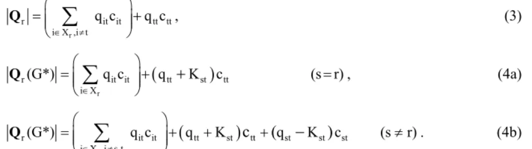
We can correct the value of qtt in the new matrix by adding Kst to it: if (s,t) doesn’t exist then Kst = +1, else Kst = –1. For the new value of qst we will have to subtract Kst , given the negative sign of qst . Then we have, with Xr = X – {r},
r
r it it tt tt
i X ,i t
q c q c
∈ ≠
= +
∑
Q , (3)
(
)
r
r it it tt st tt
i X
(G*) q c q K c (s r)
∈
= + =
∑
+Q , (4a)
(
)
r
r it it tt st tt st st st
i X ,i s,t
(G*) q c q K c (q K )c (s r)
∈ ≠
= + + + ≠
∑
−Q . (4b)
The difference between (4a-b) and (3), affected by the sign of Kst, corresponds to the
thesis.
Def. 2.4: With G = (X,U) directed (undirected), we will call Br = [brij], for every r ∈ X, the
rth-spanning arborescence pertinence matrix, r-APM (B = [bij], for any r ∈ X, the spanning
tree pertinence matrix, TPM).
Example 2.1: Let G be the graph represented in Fig. 2.1, where the alphabetic ordering of the arc labels corresponds to the lexicographic ordering of the corresponding pairs:
Fig. 2.1 – The graph G.
We have
1 -1 -1 0 0 3 1 6
0 2 -1 -1 3 0 3 0 0 1 3
-1 0 3 0 2 1 3 0 1 0 3
Q =
0 -1 -1 1
and T
1
(Q+) =
3 0 6
then B1 =
where the underlined bold entries are associated with void pairs (non-existent arcs in G). The addition of w = (1,4) to the graph, for instance, creates six new 1-SPA’s, which can be identified as acw, abw, bfw, agw, cfw and gfw. On the other hand (4,2) – that is, f – is in the graph but does not belong to any 1-SPA.
The expressions (3) and (4a-b) can be applied to undirected graphs, by considering their symmetric adjacency matrices, to obtain the TPM. But we have two differences:
• there is only one TPM B for a given graph, regardless of the choice of the root;
• the choice of a root implies a directed structure: we thus have to consider pairs of symmetric elements in order to take all tree-forming possibilities into account.
In the example below we have, for instance, b43 = 1 and b34 = 4 but we will want to find in both entries the sum corresponding to the sole structure containing (4,3) and the four structures containing (3,4).
If we then consider the symmetric graph associated with the graph of Fig. 2.1, the matrix obtained from (1a-c) will be B’ but our final answer will be B = B’ + (B’)T. Both matrices are shown below, with the entries referred to in bold underlined characters:
0 5 5 8 0 5 5 8
0 0 2 4 5 0 4 5
B’ =
0 2 0 4 B = 5 4 0 5
0 1 1 0 8 5 5 0
It is easy to calculate a reduced Laplacian determinant of the original undirected graph, whose value is 8. According to B, the addition of the edge (1,4) corresponds to 8 new trees, summing up to 16. But now we have a complete graph, for which we have the already-known result of 44 -2 = 16 trees, Harary (1971).
3. The generalization for valued graphs
Now let G = (X,U) be an arc-valued directed graph with value matrix V = [vij].
Def. 3.1: The valued Laplacian Q(G) = [qij] of a valued graph G = (X,U) is the matrix
given by
qii = ii
j i
v ≠
∑
, qij = -vij (i ≠ j).A known result (see for instance Chung & Langlands (1996)) states that, if Hr(G) is the set of r-SPA on G, then the determinant of the valued reduced Laplacian verifies that
|Qr(G)| = v
∈
∑ ∏
r ∈ ij h H (G) (i,j) h,
where the weight of any arborescence is defined as the product of the values of its arcs. (If vij = 1 for every (i,j) ∈ U we have the result already given by Theorem 2.1).
elements of Rij(r) ⊂ Hr(G). Considering the entries of Br which are associated with arcs of G, the arc counting for the entire set of spanning arborescences will be
(n – 1) |Hr(G)| = rij i, j b ∈
∑
U (5)and we have, for the corresponding total value,
v(Hr(G)) = rij ij
i, j b v ∈
∑
U (6)Now let us consider the valued graph Gst = G – (s,t) (Gst = G∪ (s,t)) and its adjacency matrix,
whose reduced Laplacian matrix will be Qstr and whose r-APM matrix we will call
st r r = β[ ij]
B . (We note that the r-APM matrix is a structural result that does not depend on arc
values). An expression similar to (6) can be derived for the total value of its r-SPA’s.
To define r-rooted spanning arborescence value matrices (r-APVM) Sr= σ[ str], r ∈ X, of the r-SPA disconnected by the removal (created by the addition) of the arc (s,t), we write
n
r r r
st st ij ij ij i, j 1
i j
K ( b )v
= ≠
σ =
∑
β − (7)where in the case of (s,t) removal (addition) we will evidently have β =str 0 r st
(b =0). The coefficient Kst has the same meaning as in the proof of Theorem 2.2.
In a similar way we can build a spanning tree value matrix (TPVM).
The counting matrices Bstr can be determined by applying Theorem 2.2, but to do that we
will need the corresponding reduced adjoint matrices (Qstr)+. Since their determinants count the number of r-rooted arborescences in the modified graphs, we have for Gst , according to (1a-c) and (2),
st st
r r st tt r r st tt st
|Q | |=Q | K c+ (s=r), |Q | |= Q | K (c+ −c ) (s≠r), (8a,b)
It follows immediately that
rt T r rt 1 T
r r rt tt r
st T r st 1 T
r r st st r
[( ) ] [ (| | K b )( ) ] , (s r)
[( ) ] [ (| | K b )( ) ] (s r).
+ −
+ −
= + =
= + ≠
Q Q Q
Q Q Q (9a,b)
if they exist: if for Kst = -1 (edge removal) and for given r, s, t we have brst=|Qr| in (8a,b),
every r-SPA will contain (s,t), then |Qstr |=0 and there will be no inverse.
We have already obtained Qr+ when calculating Br . As Qr and Qstr differ one from another by at most two elements in the same column, we can use the product form of the inverse (see for instance Hadley (1965)) to obtain the inverses (Qstr )−1 and their adjoints. To that end, we consider a transform matrix Est such that
st 1 1
r) st r
− = −
Let us express both inverses through their column vectors,
st 1 st r ([ r] )j
(
Q)
− = q , 1r ([ r j] )
− =
Q q , j ≠ r (11a,b)
On the other hand, Est can be written as
Est = ([er]1, …, [er]t-1, …, η, [er]t+1, …, [er]n), (12)
where [er]i (i ≠ r) is the ith unit column vector without the rth component and
η = [ηi], ηi = -yi / yt (i ≠ r, t), ηt = 1 / yt , (13a,b)
the vector y being given by
1 st r
[
r]
t−
=
y Q q . (14)
To calculate η,we observe that the changes brought to Qr by the addition or the removal of an arc (s,t) can be written as
st r t
[
q]
=[qr t] +K [ ]st er t (s = r) (15a)st r = Q
st r t
[
q]
=[qr t] +K ([ ]st er t−[ ] )es t (s ≠ r) (15b)Then, premultiplying (15a,b) by r1
−
Q we obtain, for the tth column,
=[ ]er t+K [st qr]t (s = r) (16a)
1 st r [ r]t
− =
Q q
=[ ]er t+K ([st qr t] −[qr s] ) (s ≠ r) (16b)
According to (14), the first member of these equations is equal to y; then, from (16a,b) we have
yi = Kstqit (i ≠ r, t) and yt = 1 + Kstqtt (s = r) (17a)
and
yi = Kst(qit - qis) (i ≠ r, t) and yi = 1 + Kst(qtt - qts) (s ≠ r). (17b)
Then, with (14) we obtain
ηi = -Kstqit / (1 + Kstqtt) (i ≠ t), ηt = 1 / (1 + Kstqtt) (s = r) (18a) ηi = -Kst(qit - qis) / (1 + Kst(qtt - qts)) (i ≠ t), ηt = 1 / (1 + Kst(qtt - qts)) (s ≠ r) (18b)
and finally, from (10) and (12),
i
st
ij ij tj
q =q +q η (i,j ≠ r; i ≠ t) (19a)
st tj tj t
q =q η (j ≠ r), (19b)
These expressions cannot be used in the removal case for any arc (s,t) such that brst = |Qr |, as already discussed: in this case we will have, from (6),
r st
σ = rij ij (i, j) U
b v ∈
∑
.For undirected graphs, the change in the original Laplacian affects the columns s and t: we thus have to use the proper indexing to apply the procedure once more.
The complexity
The most time-consuming operations in the process are those associated with matrix inversions and products, which are at most O(n3). Each root r in a directed graph requires at most O(n3) operations for its r-APM to be obtained. (The same is required for the TPM of an undirected graph). These exigencies apply to each vertex pair (i,j) such that i ≠ j and j ≠ r for the determination of the r-APVM’s and, as a consequence, of the TPVM. Therefore the complexity in this last case is O(mn3).
4. Some examples
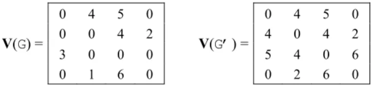
Example 4.1: Let us consider the following value matrices for the graph of Fig. 2.1 (which we will now denote G, since it is now arc-valued) and for the corresponding undirected graph
G’:
0 4 5 0 0 4 5 0
0 0 4 2 4 0 4 2
V(G) =
3 0 0 0 V(G’) = 5 4 0 6
0 1 6 0 0 2 6 0
Let s = r = 1. To find S1 entries, we will first work by inspection.
The counting of 1-SPA given by Theorem 2.2 gives us |Q1| = 3. The three arborescences, with the values corresponding to V(G) and their total weights, are shown in Fig. 4.1 below:
(11) (10) (12)
Fig. 4.1 – The 1-SPA in G.
4 4 4
4
2
5
2 2 6
1
1 1
2 2
2 3 3 3
4 4
We have, from (5) and (6), with B1 as from Example 2.1,
(n – 1) |Hr(G)| = rij (i, j) U
b ∈
∑
= 3 + 1 + 1 + 3 + 1 = (3 x 3) = 9,v(Hr(G)) = ijr ij
(i, j) U
b v ∈
∑
= (3 x 4) + (1 x 5) + (1 x 4) + (3 x 2) + (1 x 6) = 33.We can see that this value is the total value of the nine arcs in Fig. 4.1, as 11 + 10 + 12 = 33.
The arcs (1,2) and (2,4) belong to every 1-SPA, so their removal values are equal to this last result,
1 1
12 24 .
σ =σ =33
It is easy to find the remaining removal values, σ113=11,σ123=10,σ142=0, σ143=12: we can see that each one of these arcs belongs to a single arborescence.
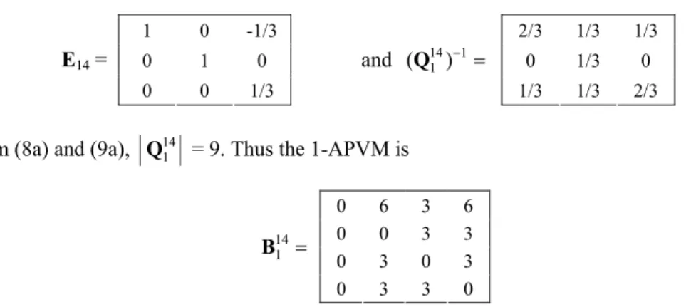
We will next examine the case of (s,t) = (1,4) ∉ U addition to G, now working with the algebraic technique already discussed. We will be assigning the weight 1 to the new arcs.
Here s = r = 1: with [q1]4 = [-1, 0, 1 ] and K14= +1 we apply (19a) to obtain η = [-1/3, 0, 1/3 ]. Thus with t = 4, we have
1 0 -1/3 2/3 1/3 1/3
0 1 0 0 1/3 0
E14 =
0 0 1/3
and (Q141 )−1=
1/3 1/3 2/3
From (8a) and (9a), 14 1
Q = 9. Thus the 1-APVM is
0 6 3 6 0 0 3 3 0 3 0 3 14
1 = B
0 3 3 0
We already have B1 from Example 2.2. Applying (7) with b114= 0 we obtain for (i,j) ∈ U, a
total weight of σ114= 51. It is easy to verify that this value corresponds to the 6 new arborescences in Fig. 4.2, where (1,4) is dashed and the arc orientations are to be taken from the root (in white) on.
For the addition of (3,2) to G we obtain one new arborescence, ((1,3),(3,2),(2,4)) with value 8 and for that of (3,4) (also to the original G), three new arborescences are created, with total value 9 + 7 + 10 = 26.
The complete 1-APVM for this graph is S1 and the corresponding TPVM, obtained as
already discussed, is S1' below:
0 33 11 51 0 62 65 75
0 0 10 33 62 0 50 57
0 8 0 26 , ' 1 S =
65 50 0 69 S1=
0 0 12 0 75 57 69 0
Example 4.2:
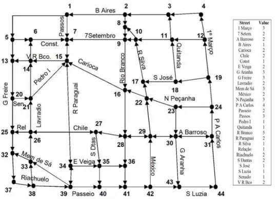
We will consider a subset of the central region of the city of Rio de Janeiro, represented by a directed graph where we might be interested in studying the impact on traffic of blocking off a given street, for public works or as a consequence of an accident. The vertices will be associated with the corners and the arcs with street segments between two corners, with the direction corresponding to the traffic flow, as in Fig. 4.3 below:
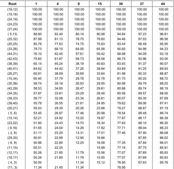
Table 4.1 – Percentual participation of arcs in arborescences with given roots.
Root 1 4 9 15 30 37 44
(19,12) 100.00 100.00 100.00 100.00 100.00 100.00 100.00 (19,18) 100.00 100.00 100.00 100.00 100.00 100.00 100.00 (24,19) 100.00 100.00 100.00 100.00 100.00 100.00 100.00 (24,23) 100.00 100.00 100.00 100.00 100.00 100.00 100.00 (31,24) 100.00 100.00 100.00 100.00 100.00 100.00 100.00
( 5,13) 88.80 82.40 80.14 80.98 94.84 97.23 96.81 (25,32) 87.99 81.13 78.70 79.60 94.46 97.03 96.58 (20,25) 85.76 77.63 74.75 75.83 93.44 96.48 95.95 (33,26) 79.73 68.15 64.05 65.58 90.65 94.98 94.23 (44,31) 76.10 62.45 57.61 59.42 88.98 94.09 93.19 (42,43) 75.60 61.67 56.73 58.58 88.75 93.96 93.05 (38,39) 65.14 45.24 38.19 40.83 83.93 91.37 90.07 (40,41) 64.62 44.42 37.26 39.94 83.69 91.25 89.93 (26,27) 60.91 38.59 30.69 33.64 81.98 90.33 88.87 (15,34) 60.40 37.79 29.78 32.78 81.75 90.20 88.72 (35,36) 58.74 35.18 26.83 29.95 80.98 89.79 88.25 (42,29) 58.53 34.85 26.47 29.61 80.88 89.74 88.19 (34,35) 57.87 33.81 25.29 28.48 80.58 89.57 88.00 (39,33) 56.77 32.08 23.34 26.61 80.07 89.30 87.69 (39,40) 55.79 30.55 21.61 24.95 79.62 89.06 87.41 (20,21) 55.03 29.35 20.26 23.66 79.27 88.87 87.19 ( 5, 6) 53.45 26.87 17.46 20.98 78.54 88.48 86.74 (15,14) 52.21 24.92 15.25 18.87 77.97 88.17 86.39 (23,22) 51.90 24.43 14.70 18.34 77.83 88.10 86.30 ( 9,16) 51.65 24.04 14.26 17.92 77.71 88.04 86.23 ( 2, 8) 51.11 23.20 13.31 17.01 77.46 87.90 86.08 (29,30) 50.91 22.88 12.95 16.66 87.85 86.02 ( 8, 9) 50.86 22.80 12.25 16.58 77.35 87.84 86.01 (11,10) 50.51 22.25 15.99 77.19 87.75 85.91 (12,11) 50.26 21.85 11.79 15.56 77.07 87.69 85.83 (18,17) 50.26 21.85 11.79 15.55 77.07 87.69 85.83 ( 4, 3) 50.00 11.34 15.12 76.95 87.63 85.76 (11, 3) 11.34 21.45 11.34 76.95
The figure shows the graph and a table with weights given to different streets according to their importance to traffic flow. Pedestrian-only streets were suppressed. Table 4.1 shows the percentual values of the participation of some arcs in sets of arborescences with given roots. It is interesting to note that the arcs are chiefly the same in the examples shown, but the percentual values show significant changes from one root to another. This table does not include arcs (e.g. (1,5)) which are the unique exit for a vertex as they obviously belong to every partial arborescence.
Example 4.3:
Fig. 4.4 – The TRANSPAC network.
Here we are interested both in the effect of an eventual edge failure and in the gain one could obtain by building a new connection. The evaluative measure in both cases will be the number of spanning trees associated with the concerned edge, which belongs to the network in the first case and is projected to be built in the second case.
Tables 4.2 and 4.3 below show, respectively, the number of spanning trees associated with fifty vertex pairs, both in the first and in the second case.
Table 4.2 – Percentual increase in number of spanning trees associated with a new edge.
Edge % increase Edge % increase Edge % increase Edge % increase Edge % increase
Table 4.3 – Percentual removal of spanning trees associated with a removed edge.
Edge % removal Edge % removal Edge % removal Edge % removal Edge % removal
(10,22) 89.66 (14,17) 82.48 (26,14) 80.00 (27,10) 78.15 (14, 9) 76.37
(14,10) 88.88 (23,18) 82.07 (26,18) 79.51 (25,14) 78.13 ( 7,10) 76.33 (18,10) 88.08 (18,17) 81.29 ( 9,10) 79.49 (23,17) 77.92 ( 4,14) 76.32
(10,17) 86.89 (23,22) 81.06 (24,10) 79.49 (18,15) 77.73 (18, 9) 75.95
(14,22) 85.90 (22,26) 81.03 (24,22) 79.06 (11,10) 77.47 (15, 9) 75.83
(14,18) 85.85 (14,23) 80.89 (15,14) 78.98 (25,18) 77.27 (12,22) 75.26
(18,22) 85.06 (10,28) 80.54 (10, 4) 78.97 (12,10) 77.23 (18, 4) 75.24 (22,17) 84.56 (25,10) 80.45 (22,25) 78.47 (23,26) 76.66 (22,11) 75.03
(10,23) 83.45 ( 2,10) 80.30 (10,15) 78.39 (28,17) 76.63 (17,24) 75.03
(10,26) 82.60 (22,28) 80.17 (28,14) 78.23 (22,27) 76.47 (17, 2) 75.01
We can see that a number of the pairs giving a strong increase in the number of spanning trees contain 2-degree vertices, which can be easily associated with the level of connectivity. From these it is interesting to observe that 1 and 3 are geographically near one another. Thus the building of an edge (1,3) should therefore have a good cost-benefit ratio, since it would increase the number of spanning trees in the graph by a factor of 2.82.
On the other hand, the most critical edge in terms of failure is (10,22), which has value 3 and connects two high-degree points (10 is Paris). The participation of vertices in pairs which are important both for building new edges and in terms of edge failures is given by Table 4.4.
Table 4.4 – Participation of vertices in important pairs.
Vertex contribution for important new edges Vertex participation in failure-critical edges
1 12 8 14 15 0 22 0 1 6 8 7 15 0 22 8 2 0 9 0 16 12 23 0 2 1 9 1 16 6 23 4 3 12 10 0 17 0 24 0 3 6 10 11 17 4 24 2 4 0 11 0 18 0 25 0 4 0 11 0 18 6 25 1 5 0 12 0 19 0 26 0 5 0 12 0 19 0 26 4 6 12 13 10 20 14 27 0 6 6 13 5 20 7 27 0 7 0 14 0 21 14 28 0 7 0 14 6 21 7 28 2
5. Conclusions
In this work, we have presented a technique for evaluating the relative importance of the edges in a directed (undirected) edge-weighted graph by using as a criterion the weights of the spanning arborescences (spanning trees) associated with each pair of vertices, as defined in the text. We consider this criterion to be a useful tool for ranking both existent edges according to the importance of their eventual failure in a network, and non-existent edges according to their positive influence within the planning of network improvements.
Acknowledgments
For the support for this work, we are indebted to Laboratoire PRiSM of Versailles University in St. Quentin-on-Yvelines, particularly to Professor Catherine Roucairol.
We are also indebted to CNPq (Brazilian Council for Scientific and Technological Development) for their financial support of our visit to PRiSM.
References
(1) Berge, C. (1973). Graphes et hypergraphes. Dunod, Paris.
(2) Berman, K.A. (1980). A proof of Tutte’s trinity theorem and a new determinant
formula. SIAM Journal on Algebraic and Discrete Methods, 1(1), 64-69, Society for Industrial and Applied Mathematics.
(3) Bott, R. & Mayberry, J. (1954). Matrices and trees. In: Economic activity analysis [edited by O. Morgenstern], John Wiley and Sons, New York, 391-340.
(4) Brown, T.J.N.; Mallion, R.B.; Pollak, P. & Roth, A. (1996). Some methods for
counting the spanning trees in labelled molecular graphs, examined in relation to certain fullerenes. Discrete Applied Mathematics, 67, 51-66.
(5) Broder, A.Z. & Mayr, E.W. (1997). Counting minimum weight spanning trees. Journal of Algorithms, 24, 171-176.
(6) Boaventura-Netto, P.O. (1984). La différence d’un arc et le nombre d’arborescences
partielles d’un graphe. Pesquisa Operacional, 4(2), 12-20.
(7) Bulteau, S. (1997). Étude topologique des réseaux de communication: fiabilité et
vulnerabilité. D.Sc. Thesis, University of Rennes 1, France.
(8) Chung, F.R.K. & Langlands, R.P. (1996). A combinatorial Laplacian with vertex
weights. Journal of Combinatorial Theory (A), 75, 316-327.
(9) Colburn, C.J.; Myrwold, W.J. & Neufeld, E. (1996). Two algorithms for unranking arborescences. Journal of Algorithms, 20, 268-281.
(10) Fard, N. & Lee, T.H. (2001). Spanning tree approach in all-terminal network reliability expansion. Computer Communications, 24(13), 1348-1353.
(11) Gross, J.L. & Yellen, J. (2005). Graph theory and its applications. 2nd ed., Chapman & Hall / CRC.
(12) Hadley, G. (1965). Linear Algebra. Addison-Wesley, Reading, New York, London.
(13) Harary, F. (1971). Graph Theory. Addison-Wesley, Reading, New York, London.
(14) Hassin, R. & Tamir, A. (1995). On the minimum diameter spanning tree problem.
Information Processing Letters, 53, 109-111.
(16) Kelmans, A.K. (1997). Transformations of a graph increasing its Laplacian polynomial and number of spanning trees. European Journal of Combinatorics, 18, 35-48.
(17) Liang, W. (2001). Finding the k most vital edges with respect to minimum spanning
trees for fixed k. Discrete Applied Mathematics, 113, 319-327.
(18) Serdjukov, A.I. (2001). On finding a maximum spanning tree of bounded radius.
Discrete Applied Mathematics, 114, 249-253.