doi: 10.1590/0101-7438.2015.035.02.0423
SOME ILLUSTRATIVE EXAMPLES ON THE USE OF HASH TABLES
Lucila Maria de Souza Bento
1, Vin´ıcius Gusm˜ao Pereira de S´a
1*and Jayme Luiz Szwarcfiter
2Received February 28, 2013 / Accepted January 13, 2015
ABSTRACT. Hash tables are among the most important data structures known to mankind. Through hashing, the address of each stored object is calculated as a function of the object’s contents. Because they do not require exorbitant space and, in practice, allow for constant-time dictionary operations (insertion, lookup, deletion), hash tables are often employed in the indexation of large amounts of data. Nevertheless, there are numerous problems of somewhat different nature that can be solved in elegant fashion using hash-ing, with significant economy of time and space. The purpose of this paper is to reinforce the applicability of such technique in the area of Operations Research and to stimulate further reading, for which adequate references are given. To our knowledge, the proposed solutions to the problems presented herein have never appeared in the literature, and some of the problems are novel themselves.
Keywords: hash tables, efficient algorithms, practical algorithms, average-time complexity.
1 INTRODUCTION
Choosing the most appropriate algorithm for a problem requires awareness with a number of data structures and general computational techniques that may be used to actually implement the algorithm in some programming language. In a paper entitled “Data Structures and Computer Science Techniques in Operations Research” [8], Fox discussed some applications of existing algorithms and techniques – such as heaps, divide-and-conquer and balanced trees – to well-known operational research problems including incremental allocation, event lists in simulations, and thekth shortest path. The present paper pursues a similar goal, albeit focusing on a specific technique that has over the years gained increasing attention in Computer Science in general:
hashing.
*Corresponding author.
1Department of Computer Science, Institute of Mathematics, Federal University of Rio de Janeiro, 21941-590 Rio de Janeiro, RJ, Brazil. E-mails: [email protected]; [email protected]
The hashing technique provides a way to store and retrieve data that is efficient in both time and space. Basic theory can be found, for instance, in [4]. Numerous recent publications deal with the technical aspects of hashing implementations, exploring new ways to solve its intrinsic problems such as handling collisions, devising nearly ideal hash functions and improving their performance in a number of ways. Among them, we cite the work on perfect hash functions and dynamic perfect hashing in [7, 5], the cuckoo hashing technique [25], the work on uniform hashing in [24] and the ingenious use of random hypergraphs in perfect hashing described in [2]. A recent trend is the use of machine learning tools to devise good hash functions [26, 17, 28, 9, 23, 20]. Other recent publications include [12, 1, 13, 19].
The hashing technique is widely used nowadays in database indexing, compiler design, caching, password authentication, software integrity verification, error-checking, and many other applica-tions. Still, a seemingly uncountable number of further problems do allow for efficient, practical algorithms through the use of hashing.
Some aspects of hashing have already been discussed in the Operations Research literature, and hashing-based improvements for known Operations Research problems are indeed not rare. See, for instance, [14, 29, 3]. We believe, however, that the full potential of hashing has yet to be explored in the field, allowing for plenty of further improvements.
After briefly revisiting some concepts related to hashing (Section 2), we focus on a number of applications (Sections 3.1–3.5), illustrating how it can be successfully employed in conceiving efficient solutions to problems that might not suggest its use at first glance. Though it is certainly possible to find several much more complicated examples where hash tables may come in handy in a less-than-obvious way, we selected but a few simple problems. We believe the examples provided are sufficiently illustrative and dispense with otherwise naive attempts to categorize exhaustively the cases in which the hashing technique could and should be considered.
The problems presented in Sections 3.2, 3.3 and 3.5 are original. Likewise, the solutions pro-posed in this text are all, to our knowledge, yet unpublished.
2 HASHING
The central idea of the hashing technique is to use ahash functionto translate a unique identifier (orkey) belonging to some relatively large domain into a number from a range that is relatively small [18]. Such number corresponds to the memory address (basically the position in a “table”, thehash table) in which theobject– usually a (key, value) entry, where the value can be of any data type – should be stored. Owing to the key-value mapping it provides, a hash table is usually called a hash map. Sometimes, though, the object to be stored is but the key itself. In these cases, the hash table is often referred to as ahash set.
is not known beforehand, it may not be possible to define such a perfectly injective function, hence the same position in a hash table may be assigned to different keys in a situation known ascollision.
When collisions occur, it is necessary to store the objects with colliding keys in alternative po-sitions [16]. Among the most widely adopted methods for resolving collisions is the method of
chaining, in which the hash table positios are regarded asbuckets, each one containing a pointer to a linked list (or other data structure) where the colliding objects will be located. It is a simple exercise to show that the average number of elements in each bucket is equal to theload factor
of the hash table, defined asα=n/mfor a hash table withmpositions andnstored objects. The actual complexities of searches, insertions and deletions depend on the choice of the hash function (as well as on the load factor). Because good hash functions are known for the vast ma-jority of data types, thesimple uniform hashing assumption(SUHA), whereby the distribution of keys into buckets approaches a uniform distribution, is often a reasonable premise. The average case analysis in algorithms that involve hashing can therefore rely on the SUHA and still provide a fairly accurate indicator of their practical performances.
By using a hash function which disperses the keys with near uniform distribution along the buckets, and provided the load factor never exceeds a certain constant (which is achieved simply by dimensioning the hash table proportionally to the number of objects to be stored), it can be shown that those operations are performed inO(1)time, on average [4]. Even though a “bad” instance may demand some worst-case performance that is quite poorer than the average, the probability of its occurrence is usually extremely low, resulting from an unbelievably unfortunate choice of the hash function.
It is certainly not in the scope of this text the design of hash functions that are most appropriate to each case, a subject that requires statistical tools and specific study [15]. The algorithms pre-sented in this paper, however, do not depend upon complicated, custom-tailored hash functions. Backed by the SUHA, we assume the existence of a near-uniform hash function that maps each key onto a number in the range[0,m−1], wheremis the size of the hash table. Indeed, the vast majority of modern programming languages provides efficient inbuilt implementations of hash tables, so the basic hashing operations, and collision handling, and even the choice of hash functions become totally transparent to the programmer. In other words, it isnotnecessary to even think about the low-level details of the technique — the programmer is free to concentrate on the algorithm itself. Such is the focus of this paper.
In the next sections, we look into some examples of hashing in action.
3 ILLUSTRATIVE EXAMPLES
3.1 The Pair Sum Problem
Given an integerkand a listAofnunordered integers, find out whether there is a pair{x,y} ⊂ A
Unlike the Subset Sum Problem, which is NP-hard and admits a number of interesting approx-imation algorithms [21], the Pair Sum Problem is clearly polynomial. For a naive solution, just check all pairs(x,y) of elements of A. If x+ yequals k, returnyesand stop. Although no extra space is required, the number of additions and comparisons to be performed is O(n2)in the worst case.
We want to do better. First note that, if we select an element xof A, we can look for its com-plement y = k−x in A, and the problem is now a search problem. If, for each x, we need to traverse the whole list to check whether it contains its complement, then our algorithm still demands O(n2)time. A better alternative would be to first sort the list A, and then, for each
x ∈ A, look for its complement using binary search, whereupon our time complexity would be
O(nlogn).
In the pursuit of a linear-time algorithm, we could try and use a boolean array to represent the elements of A: the ith position of the array contains a ‘1’ (or ‘true’) if and only ifi ∈ A. Each complement could then be looked for in constant time. However, suchdirect addressing
approach, in which the address of the data related to some keyiis exactlyi, has a serious caveat: the space allocated for object storage must be at least as large as the maximum possible key. In other words, the length of our boolean array would depend on themaximum elementwofA, not on the sizenofA. Sincewcan be represented by log2wbits, that means exponential space. We can use a hash set to store the elements of A. The amount of space we need is that to store
nintegers (scattered along their respective buckets) plus an underlying array withn/αpositions. For a constant load factorα, that means O(n)space, while the average time of all dictionary op-erations is as good as O(1)under the simple uniform hashing assumption. The overall expected time of such algorithm –“for each elementxin the list, ifk−yis in the (initially empty) hash set
H, then returnyes, otherwise insertxinH”– is therefore alsoO(n), corresponding to theO(n)
insertions and lookups in the hash set, in the worst case.
A similar approach can be used to determine the intersection of two listsA,B. Create a hash set
H and populate it using the elements of one of the lists, say A. Next, for each elementx ∈ B, look forxinH, for an expected(|A| + |B|)overall time.
3.2 The Sum of Functions Problem
Given a set Aand a function f, whose domain containsAand which can be calculated in time
O(1), find all non-trivial quadruples(x,y,z, w)of elementsx,y,z, w ∈ Asuch that f(x)+ f(y)= f(z)+ f(w).
For a trivial solution, we may simply test each quadruple of distinct elements of the set A. We can do this in(n4)time, wheren = |A|.
A more efficient solution can be achieved by sorting. Pick all pairs(x,y)⊂ A, put them on a listL, and sort them bydx,y = f(x)+ f(y). Now, all pairs of elements whose images under f
input : arrayA, functionf
output: all (x, y, z, w)⊂Asatisfyingf(x) +f(y) =f(z) +f(w)
H←a hash map with size|A|2
foreach(x, y)⊂Ado d←f(x) +f(y)
if dis a key stored inH then
Sd←H.get(d) // the value stored withdinH else
Sd← {(x, y)} insert (d, Sd) inH end
Sd←Sd∪ {(x, y)} end
foreach(d, Sd)∈H do foreach(x, y)∈Sddo
foreach(z, w)∈Sd\ {(x, y)}do print (x, y, z, w)
end end end
Algorithm 1–Sum Functions(A,f).
combined to produce the intended quadruples in constant time per quadruple. Owing to sorting, the overall time complexity of this approach isO(n2logn+q), in the worst case, whereqis the number of quadruples in the output.3
Now we look into a hashing-based approach. We start with an empty hash mapH. We consider each unordered pair(x,y)of distinct elements of A, obtainingd = f(x)+ f(y), one pair at a time. Ifd isnota key stored in H, we insert the (key, value) pair(d,Sd)inH, whereSdis
a collection (which can be implemented as a linked list, a hash set or whatever other structure) containing only the pair(x,y)initially. On the other hand, ifd is already stored inH, then we simply add(x,y)to the non-empty collectionSdwhichd already maps to inH. After all pairs
of distinct elements have been considered, our hash map will contain non-empty collectionsSd
whose elements are pairs(x,y)satisfying f(x)+f(y)=d. For each non-unitary collectionSd,
we combine distinct pairs(x,y), (z, w)∈ Sd, two at a time, to produce our desired quadruples (x,y,z, w).
The pseudocode of the proposed hash-based solution is given as Algorithm 1.
As for the time complexity of the algorithm, each keydcan be located or inserted inHinO(1)
average time, and each of the(n2)pairs(x,y)of elements ofAcan be inserted in some listSd
inO(1)time (assuming, for instance, a linked list implementation forSd). Thus, the whole step
of populatingHcan be performed in(n2)time on average. Now, each of theqquadruples that satisfy the equality can be obtained, by combining pairs in a same list, inO(1)time. Thus, the whole algorithm runs in(n2+q)expected time.
If we tried to achieve the same performance by using an array and direct addressing, such array would have to be twice as large as the maximum element in the image of f. The use of hashing avoids that issue seamlessly.
3.3 The Permutation Bingo Problem
In the standard game of bingo, each of the contestants receives a card with some integers. The integers in each card constitute a subset of a rather small range A = [1,a]. Then, subsequent numbers are drawn at random from A, without replacement, until all numbers in the card of a contestant have been drawn. That contestant wins the prize.
In our variation of the game, the contestants receive an empty card. Subsequent numbers are drawn at random from some unknown, huge range B = [1,b],with replacement, forming a sequenceS. The contestant who wins the game is the one who first spots a setW = {x,y,z}
of three distinct numbers such that all 3! = 6 permutations of its elements appear among the subsequences of three consecutive elements ofS. As an example, the sequence
S =
2,19,4,1,100,1,4,19,1,4,1,19,100,192,100,4,19,2,1,19,4
is a minimal winning sequence. There is a set, namely W = {1,4,19}, such that every per-mutation ofW appears as three consecutive elements ofS. Even though the setB is huge, the distribution of the drawing probability alongBis not uniform, and the game finishes in reason-able time almost surely.
We want to write a program to play the permutation bingo. Moreover, we want our program to win the game when it plays against other programs. In other words, we need an efficient algorithm to check, after each number is added toS, whetherShappens to be a winning sequence. One possible approach would be as follows. Keep S in memory all the time. After the n-th number is added, for alln ≥8 (a trivial lower bound for the size of a winning sequence), traverse
S = (s1,s2, . . . ,sn)entirely for each set Ri = {si,si+1,si+2} of three consecutive distinct elements (with 1≤i ≤ n−2), checking whether all permutations ofRi appear as consecutive
sn is added, we can keep the bins in memory and proceed to place only each freshly formed
subsequence(sn−2,sn−1,sn)into the appropriate bin – an approach which also allows us to keep
but the two last elements ofSin memory.
We still have a big problem, though. Given a label, how to find the bin among the (possibly huge number of) existing bins? If we maintain, say, an array of bins, then we will have to traverse that entire array until we find the desired bin. It is not even possible to attempt direct addressing here, for the rangeB of the numbers that can be drawn is not only unknown but also possibly huge – let alone the number of subsets of three such numbers! Even if we did knowB, there would probably not be enough available memory for such an array. We know, however, that the game always ends in reasonable time, owing to an appropriate probability distribution alongB
enforced by the game dealer. Thus, the actual number of bins that willeverbe used is small, and available memory to store onlythatnumber of bins shall not be an issue. We can therefore keep the bins in a linked list, or even in an array without direct addressing. When the sequence has sizen, such list (or array) of bins will have size O(n), and the time it takes to traverse it all and find the desired bin will also beO(n).
The use of hashing can improve the performance even further. We use a hash map where the keys are the bin labels and the values are the bins themselves (each one a list, or bit array etc.), so every time a new element is added, we can find the appropriate bin and update its contents in expected constant time. Since we do not know the number of bins that will be stored in our hash map throughout the game, and we want to keep the load factor of the hash map below a certain constant, we implement the hash map over an initially small dynamic array and adopt a geometric expansion policy [10] to resize it whenever necessary. By doing this, the amortized cost of inserting each new bin is also constant, and the algorithm processes each drawn number in overallO(1)expected time.
3.4 The Ferry Loading Problem
The Ferry Loading Problem (FLP) is not unknown to those used to international programming competitions. It appears in [27] in the chapter devoted to dynamic programming, the technique employed in the generally accepted, pseudo-polynomial solution. By using a clever backtracking approach aided by hashing, we obtain a simpler algorithm which is just as efficient, in the worst case. As a matter of fact, our algorithm may demand significantly less time and space, in practice, than the usual dynamic programming approach.
There is a ferry to transport cars across a river. The ferry comprises two lanes of cars throughout its length. Before boarding on the ferry, the cars wait on a single queue in their order of arrival. When boarding, each car goes either to the left or to the right lane at the discretion of the ferry operator. Whenever the next car in the queue cannot be boarded on either lane, the ferry departs, and all cars still in the queue should wait for the next ferry. Given the lengthL ∈Zof the ferry and the lengthsℓi ∈Zof all carsi>0 in the queue, the problem asks for the maximum number
A brute force approach could be as follows. Starting fromk=1, attempt all 2k distributions of the firstkcars in the queue. If it is possible to loadkcars on the ferry, proceed with the next value ofk. Stop when there is no feasible distribution of cars for somek. Clearly, if the numbernof cars loaded in the optimal solution is not ridiculously small, such an exponential-time algorithm is doomed to run for ages.
A dynamic programming strategy can be devised to solve the FLP in(n L)time and space. This is not surprising, given the similarity of this problem with the Knapsack Problem [30], the Partition Problem [11], and the Bin Packing Problem [6]. Such complexity, as usual, corresponds to the size of the dynamic programming table that must be filled with answers to subproblems, each one computed in constant time.
Apart from the dynamic programming approach, one could come up with a simple backtracking strategy as follows. Identify each feasible configuration ofkcars by a tuple(x1, . . . ,xk), where xi ∈ {left,right}indicates the lane occupied by theith car, fori =1, . . . ,k. Each configuration (x1, . . . ,xk) leads to configurations(x1, . . . ,xk, left) and (x1, . . . ,xk, right), respectively, if
there is room for the(k+1)th car on the corresponding lane. Starting from the configuration (left) – the first car boards on the left lane, without loss of generality –, inspect all feasible configurations in backtracking fashion and report the size of the largest configuration that is found. It works fine. Unfortunately, such approach demands exponential time in the worst case.
However, we can perfectly well identify each configuration by a pair (k,s), wherekis the num-ber of cars on the ferry ands is the total length of theleft lanethat is occupied by cars. Each configuration (k,s)leads to at most two other configurations in the implicit backtracking graph:
• (k+1,s+ℓk+1), by placing the(k+1)th car in the left lane, which is only possible if
s+ℓk+1≤L; and
• (k + 1, ℓ), by placing the (k +1)th car in the right lane, which is only possible if
k+1
i=1ℓi
−s≤L.
If neither placement of the(k+1)th car is possible, backtrack. Notice that a same configuration
(k+1,s′)may be reached by two distinct configurations(k,s1)and(k,s2). It happens precisely if|s1−s2| =ℓk+1. However, we do not want to visit a same configuration twice, and therefore
we must keep track of the visited configurations.
The algorithm searches the whole backtracking graph, starting by the root node(0,0)– there are zero cars on the ferry, initially, occupying zero space on the left lane. The reported solution will be the largestkthat is found among the visited configurations(k,s).
As for the time complexity, the whole search runs in time proportional to the number of nodes (configurations) in the backtracking graph. Since 0 ≤k ≤n, 0≤ s≤ L, and bothkandsare integers, such number is O(n L), bounding the worst-case time complexity of our algorithmif
use a 2-dimensional matrix to store the configurations, the problem is solved. However, by doing so, we demand(n L)space, even though our matrix will most likely be absolutely sparse.
We can resort to hashing to solve that. By using a hash set to store the visited configurations, we can still perform each configuration lookup in (expected) constant time, and the required space will be proportional to the numberO(n L)of configurations that are actually visited during the search. In practice, the O(n L)time and space required by our algorithm can be remarkably smaller than the(n L)time and space of the dynamic programming solution, specially if there are many cars with the same size.
3.5 The Trading Company Problem
Considerer the following hypothetical problem. A certain company X operates in the stock market, entering a huge number of financial transactions – calledtrades – every day. On the other side of each trade, there is some companyY, call it acounterpartyofX. To each trade of
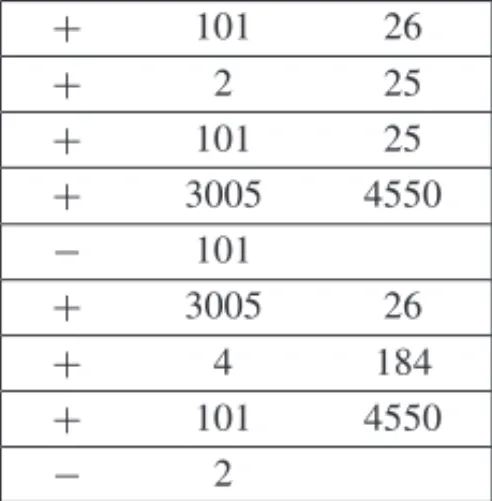
X is assigned aportfolionumber, which isnota unique identifier of the trade, and is not even unique per counterparty. In other words, trades with different counterparties may be assigned the same portfolio, and different trades with the same counterparty may be assigned distinct portfo-lios as well, according to some internal policy of the company. WheneverX enters into a trade, a new line such as “+101 25” is appended to a log file, where “+” indicates that a new trade was initiated by X, “101” is the counterparty id, and “26” is the portfolio of that trade. At any time during a typical day, however, a counterpartyY may withdraw all transactions withX. FromX’s standpoint, that means all trades it had entered into withYthat day are now considered void, and a line such as “−101” is logged. Here, the “−” sign indicates that a cancelation took place, and “101” is the id of the counterparty the cancelation refers to. Table 1 illustrates the basic structure of the log file ofX.
Table 1– Sample log file.
+ 101 26
+ 2 25
+ 101 25
+ 3005 4550
− 101
+ 3005 26
+ 4 184
+ 101 4550
− 2
Hash set. As usual, it is easy to think of different ways to process the file and come up with the desired information. For example, we can traverse the file in a top-down fashion (i.e. in chronological order), and, for each line “+Y P”, we check whether there is any line below it (i.e. logged after it) indicating the cancelation of previous trades withY. In case there is no such line, addPto a list of active portfolios, taking care not to add the same portfolio twice to the list. To avoid duplicates, one can already think of using a hash set, where portfolios are inserted only if they are not there already, something that can be verified in constant time, on average. This approach surely works, and it is easy to see that the time complexity of this strategy is(n2), wherendenotes the number of lines in the log file.
Yet the file can be really huge, and determining the active portfolios is a time-critical operation forX. A quadratic-time algorithm is not good enough.
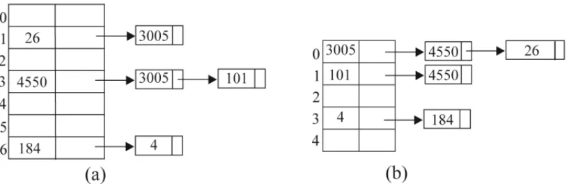
Two mirroring hash maps. Consider the use of two hash maps, this time: (i) The first one will hold a counterparties-by-portfolio map: the keys are portfolio numbers, and the value stored with each key Pis a list containing the counterpartiesY ofXfor which there are active negotiations under that portfolioP. (ii) The second is a portfolios-by-counterparty hash map: the keys are the counterparties of X, and the values associated with each counterpartyY is a list containing the portfolios assigned to active negotiations with that partner.
The file is traversed top-down. Each line with a “+” sign, be it “+ Y P”, triggers two updates in our data structure: the first is the inclusion ofY in the list of counterparties associated with portfolio Pin the counterparties-by-portfolio hash map (the keyP will be inserted for the first time if it is not already there); the second change is the inclusion of P in the list of portfolios associated with counterpartyY in the portfolios-by-counterparty hash map (the keyY will be first inserted for the first time if it is not already there).
Whenever a line with a “−” sign is read, be it “−Y”, we must remove all occurrences ofY
from both tables. In the second, portfolios-by-counterparty hash map,Y is the search key, hence the bucket associated toY can be determined directly by the hash function, and the list of port-folios associated toY can be retrieved (and deleted, along withY) in average time O(1). In counterparties-by-portfolio, however, Y can belong to lists associated to several distinct port-folios. To avoid traversing the lists of all portfolios, we can use the information in the first, portfolios-by-counterparty map (sure enough, before deleting the keyY) so we know beforehand which portfolios will haveY on their counterparty lists. We may thus go directly to those lists and removeY from them, without the need to go through the entire table. If the list of coun-terparties associated to a portfolioP becomes empty after the removal ofY, then we delete the portfolioPfrom that first hash map altogether.
After all lines of the file have been processed, just return the portfolios corresponding to keys that remain in the first, counterparties-by-portfolio hash map.
mentioned, collisions (as well as the choice of the hash function and other technicalities) are being taken care of by the lower level hash implementation, allowing us to focus on the high levelusageof it, as happens most of the time in practice.
Figure 1– Hash maps: (a) counterparties-by-portfolio; (b) portfolios-by-counterparty.
Determining the lists from which a certain counterpartyYmust be removed (due to a cancelation read from the file) can be made in average O(1)time per list, and each counterparty can be removed at most once for each line of the file that inserted it there. So far so good. However, in order to findY in each list (something we also need to do by the time weinsert Y, so we do not have the same counterparty appear more than once in the same list), we still need to traverse the whole list, which certainly increases the computational time. Since we wish we can cope with the whole file processing task in linear time, we must think of a remedy to this.
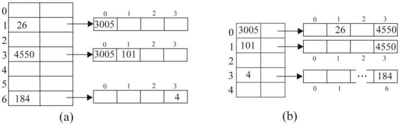
Multi-level hashing. So our problem is the time-consuming task of traversing whole lists to locate a single element. We therefore want to try and replace those lists with more performatic structures, such as binary search trees, or, better yet... hash sets! In other words, the value associated with each key P in the counterparties-by-portfolio hash map will be, instead of a list, a hash set whose keys are the ids of the counterparties associated with P (see Figure 2). The same goes for the second, portfolios-by-counter-party hash map, where portfolios will be stored in a hash set associated to each counterpartyY. Thus, counterparties and portfolios can be included and removed without the need to traverse possibly lengthy lists, but in average constant time instead. Since the cost of processing each line is now O(1)(due to a constant number of hash table dictionary operations being performed), the whole algorithm, implemented this way, runs in expected linear time in the size of the file. (Sure enough, the same time complexity could have been achieved, in the previous approach, by making a cumbersome use of pointers across the hash tables.)
Figure 2– Multi-level hashing: (a) Hash map of counterparties (represented by hash sets) per portfolio; (b) Hash map of portfolios (represented by hash sets) per counterparty.
Note that, as the file is being read upwards, the first line found with a “−” sign, be it “−Y”, indicates the cancelation of all trades company X had entered into with counterpartyY earlier in the day. Thus, such a lineLY in the log file partitions all other lines associated toY into two
groups: those which occurred chronologically before LY (and which have not been processed
yet, since they appear above it in the file), and those which occurred chronologically after LY
(and therefore have already been processed). From that moment on, the lines of the former group may be simply ignored, since the corresponding trades would not be active by the end of the day anyway. On the other hand, all lines regardingY that have already been processed (those in the latter group) correspond to trades that are active indeed by the end of the day, since they appear, in the log file, chronologically after the last cancellation involvingY.
We can therefore use again two hash sets: one for the “active portfolios”, whose keys will be returned by the end of the algorithm execution, and another for the “bypassed counterparties”, that is, the counterparties for which a cancelation line has already been read in the bottom-up traversal of the file. With such a simple structure, each “−Y” line triggers the insertion ofY into the bypassed counterparties hash set (if it is not already there), and each “+Y P” line either triggers the insertion ofPin the active portfolios hash set, in case it is not already thereand Y is not in the bypassed counterparties table; otherwise the line is ignored.
This time again, each line gives rise to a constant number of average constant-time operations, but in a much simpler fashion. The whole process runs inO(n)time, wherenis the number of lines in the log file.
4 CONCLUSIONS
The use of appropriate data structures is one of the main aspects to be considered in the design of efficient algorithms. Certain structures, however, are somewhat stigmatized, restricted to particu-lar applications and some classic variants. Though the use of hash tables in Operations Research is not new (some nice improvements based on hashing have been reported in the literature for known OR problems), we believe its possibilities are quite often neglected – or overlooked – by part of the OR community.
It is certainly important to add some creativity to one’s theoretical toolset when considering the choice of data structures. Hash tables, however, bear such an immense likelihood of producing efficient, practical algorithms, that one should always feel inclined to at least consider them, even in applications that, at a first glance, do not seem to suggest their use. In this paper, we illustrated the use of hashing to produce neat, efficient solutions to simple, didactic problems, in a selection we hope to have been as instructive as motivating.
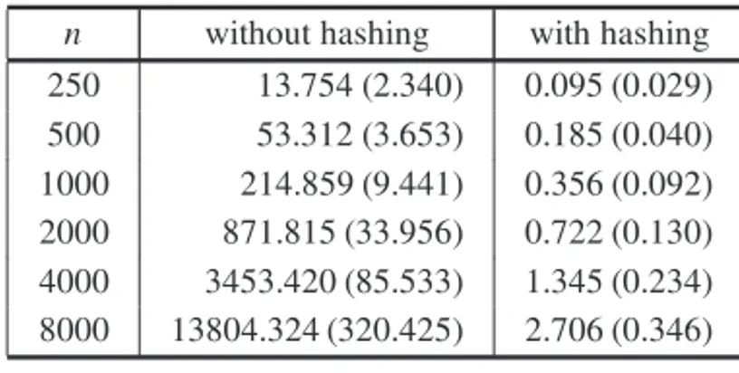
Though we have not included a whole section dedicated to computational results, implementing the algorithms we discussed is straightforward. We encourage the reader to do so, specially if he or she is not too familiar with formal complexity theory. As an example of the kind of result the reader should be able to produce, Table 2 shows a comparison between the naive algorithm and the algorithm based on hashing discussed in Section 3.1. The source code, in Python, can be found inhttps://www.dropbox.com/s/wm6goozuoq27lh6/pair_ sum.py?dl=0. It is noteworthy that the exact hash function that was used has not even be specified in the source code, which relied on inbuilt, general-purpose hash functions.4
Table 2– Average running times (and standard deviations), in mili-seconds, for input lists of sizenin the Pair Sum problem. For each value ofn, we ran the algorithms on 100 lists ofn integers chosen uniformly at random in the range[1,108].
n without hashing with hashing 250 13.754 (2.340) 0.095 (0.029) 500 53.312 (3.653) 0.185 (0.040) 1000 214.859 (9.441) 0.356 (0.092) 2000 871.815 (33.956) 0.722 (0.130) 4000 3453.420 (85.533) 1.345 (0.234) 8000 13804.324 (320.425) 2.706 (0.346)
REFERENCES
[1] ANDREEVAE, MENNINKB & PRENEELB. 2012. The parazoa family: generalizing the sponge hash functions.International Journal of Information Security,11(3): 149–165.
[2] BOTELHOFC, PAGHR & ZIVIANIN. 2007. Simple and space-efficient minimal perfect hash func-tions. In:Proc. of the 10th Workshop on Algorithms and Data Structures (WADS’07).Lecture Notes in Comp. Sc.,4619: 139–150.
[3] CHIARANDINIM & MASCIA F. 2010. A hash function breaking symmetry in partitioning prob-lems and its application to tabu search for graph coloring. Tech. Report No. TR/IRIDIA/2010-025, Universit´e Libre de Bruxelles.
[4] CORMENTH, LEISERSONCE, RIVESTRL & STEINC. 2001.Introduction to Algorithms, Vol. 2., The MIT Press.
[5] DIETZFELBINGERM. 2007. Design strategies for minimal perfect hash functions.Lecture Notes in Comp. Sc.,4665: 2–17.
[6] DOWSLAND K & DOWSLANDWB. 1992. Packing problems.European Journal of Operational Research,56(1): 2–14.
[7] DIETZFELBINGERM, KARLINAR, MEHLHORNK, MEYER AUF DERHEIDEF, ROHNERTH & TARJANRE. 1994. Dynamic perfect hashing: upper and lower bounds.SIAM J. Comput., 23(4): 738–761.
[8] FOXBL. 1978. Data Structures and Computer Science Techniques in Operations Research. Opera-tions Research,26(5): 686–717.
[9] GONG Y & LAZEBNIKS. 2011. Iterative quantization: a procrustean approach to learning bi-nary codes. In: Proc. of the 24th IEEE Conference on Computer Vision and Pattern Recognition (CVPR’11), 817–824.
[10] GOODRICHMT & TAMASSIAR. 2002.Algorithm Design: Foundations, Analysis and Internet Ex-amples, Wiley.
[11] HAYESB. 2002. The easiest hard problem.American Scientist,90(2): 113.
[12] HOFHEINZD & KILTZE. 2011. Programmable hash functions and their applications.Journal of Cryptology,25(3): 484–527.
[13] IACONOJ & P ˘ATRAS¸CUM. 2012. Using hashing to solve the dictionary problem. In: Proc. of the 23rd Annual ACM-SIAM Symposium on Discrete Algorithms (SODA’12), 570–582.
[14] JAGANNATHANR. 1991. Optimal partial-match hashing design. Operations Research Society of America (ORSA) Journal on Computing,3(2): 86–91.
[15] KNOTTGD. 1975. Hashing functions.The Computer Journal,18: 265–278.
[16] KNUTHDE. 1973.The Art of Computer Programming 3: Sorting and Searching, Vol. 1, Addison-Westley.
[17] KULISB & DARRELLT. 2009. Learning to Hash with binary reconstructive embeddings. In:Proc. of the 23rd Annual Conference on Neural Information Processing Systems (NIPS’09), 1042–1050.
[19] LI X, LIN G, SHENC, HENGEL A &VAN DEN DICKA. 2013. Learning hash functions using column generation. In:Proc. of the 30th International Conference on Machine Learning (ICML’13). Journal of Machine Learning Research,28(1): 142–150.
[20] LIUW, WANGJ, JIR, JIANGY-G & CHANGS-F. 2012. Supervised hashing with kernels. In:Proc. of the 25th IEEE Conference on Computer Vision and Pattern Recognition (CVPR’12), 2074–2081.
[21] MARTELLO S & TOTHP. 1985. Approximation schemes for the subset-sum problem: Survey and experimental analysis.European Journal of Operational Research,22(1): 56–69.
[22] MAURERWD & LEWISTG. 1975 Hash table methods.ACM Computer Surveys,7: 5–19.
[23] NOROUZIM & FLEETD. 2011. Minimal loss hashing for compact binary codes. In: Proc. of the 28th International Conference on Machine Learning (ICML’11), 353–360.
[24] PAGHA & PAGHR. 2008. Uniform hashing in constant time and optimal space.SIAM J. Comput., 38(1): 85–96.
[25] PAGHR & RODLERFF. 2004. Cuckoo hashing.J. Algorithms,51(2): 122–144.
[26] SALAKHUTDINOVR & HINTONG. 2009. Semantic hashing.International Journal of Approximate Reasoning,50(7): 969–978.
[27] SKIENASS & REVILLAMA. 2003.Programming Challenges. Springer.
[28] WANGJ, KUMARS & CHANGS-F. 2010. Sequential projection learning for hashing with compact codes. In:Proc. of the 27th International Conference on Machine Learning (ICML’10), 1127–1134.
[29] WOODRUFFDL & ZEMELE. 1993. Hashing vectors for tabu search.Annals of Operations Research, 41(2): 123–137.