Florica Novăcescu
High-performance
Scientific
Computing
using
Parallel
Computing
to
Improve
Performance
Optimization Problems
HPC (High Performance Computing) has become essential for the ac-celeration of innovation and the companies’ assistance in creating new inventions, better models and more reliable products as well as obtain-ing processes and services at low costs. The information in this paper focuses particularly on: description the field of high performance scien-tific computing, parallel computing, scientific computing, parallel com-puters, and trends in the HPC field, presented here reveal important new directions toward the realization of a high performance computational society. The practical part of the work is an example of use of the HPC tool to accelerate solving an electrostatic optimization problem using the Parallel Computing Toolbox that allows solving computational and data-intensive problems using MATLAB and Simulink on multicore and multiprocessor computers.
Keywords: HPC, parallel supercomputers, parallel computing, scientific computing
1. Introduction
The increasing requirements of computing resources have determined two di-rections of development. On the one hand, the massive parallel supercomputers which have constituted a material basis for some research centres in the world and which have represented and they still represent the actual frontier in the field of numerical simulation of different physical phenomena. The number of these com-puters is dramatically limited due to the price and the high maintenance and ex-ploitation costs, being produced in a very small bank. On the other hand, the so-called clusters (networks of computers) which represent the standard of hardware endowment for universities and research institutes, although they are composed of performant units at the level of personal computers or work stations, they
repre-ANALELE UNIVERSITĂŢII
“EFTIMIE MURGU” REŞIŢA
sent an extremely important potential of computing resources and which is hardly used in the present.
By the complexity of flow equations and the difficulties which accompany the numerical solving of mathematical models, the fluids mechanics has constituted one of the main stimulus for the development of new technics of analytic solving of equations and equations systems with partial derivatives and in the last decades, their numerical solving. The development and maturation of numeric methods and their implementation algorithms constitutes an undoubted achievement of the last two decades. Simultaneously, the available hardware resources have substantially increased the speed of calculation and the memory capacity, facilitating the current use of the numerical simulation of flows, analysis and optimization.
Therefore research and development are used in order to achieve scientific progress, for which HPC is only an instrument which is sometimes blunt, always expensive, but, however, it is an important instrument.
We live in a period interested in the use of the high performance calculation and a period with promises of unequalled performance for those who can effec-tively use the high performance computing.
2. The field of high performance computing
The work field could be translated in computing in science and engineering (CSE) or computational science and engineering (CiSE).
From the soft point of view, the high performance computing field (HPC) means the parallel computing (computer science) and the scientific computing (applied Mathematics).
The parallel computing means the simultaneous execution on several proces-sors of the same instructions with the aim to solve faster a problem, subdivided and especially adapted. The parallel computing is used for problems that require many calculations and thus, they last very long, but which can be divided in inde-pendent, simpler sub-problems [2].
Figure 1. Parallel computing.
A parallel computing system is a computer with several processors which work in parallel. The first such systems were the super-computers. The new processors of multi-core type for PCs are also parallel computing systems.
The parallel computing systems are different by their inter-connecting type which can be between the component processors (known as processing elements or PEs) and between processors and memory. Programming in parallel computing is centred on the partition of the whole problem to be solved into separate tasks, allotting the tasks to the available processors and their synchronization in order to obtain convincing results [3].
The scientific computing is based on the construction of mathematical models, quantitative analysis techniques and the use of computers in order to solve scien-tific problems [6]. It practically represents computer simulations applications and other forms of computing the problems in diverse scientific disciplines [6]. It is based on the construction of mathematical models, quantitative analysis tech-niques and the use of computers in order to analyse and solve problems. It practi-cally represents applications of computer simulations and other forms of computing the problems in diverse scientific disciplines.
The scientific computing represents the design and analysis activity for the nu-meric solving of mathematical problems in science and engineering, and tradition-ally this activity is called numeric analysis. The scientific computing is used in order to simulate natural phenomena, using virtual prototypes of models in engineering [7]. The general strategy is to replace a difficult problem with an easier one having the same solution, or a very similar solution, that is, they wish to replace an infinite problem with a finite problem, the differential one with the algebraically one, the non-linear with the linear, and eventually, a complicated one with a simple one, and the solution obtained can only approximate the solution of the original prob-lem.
3. Architecture of sequential computers. Stored-program com-puter architecture.
calculate the same result can vary from only some percents upwards, according to the way in which the algorithms are ciphered for the processor’s architecture. Ob-viously, it is not sufficient to have an algorithm and to “put them on the computer” because we should have some knowledge connected to the computer’s architec-ture and sometimes these are crucial.
Some problems can be solved on a single processor, others require a parallel computer which contains more than a processor, but taking into account the facts mentioned above, even for the parallel processing, it is necessary to understand the architecture of individual processors.
When we generally discuss about computing systems, we must take into ac-count a certain architectural concept. This concept was discovered by Turing in 1936 and it was applied for the first time in a real machine (EDVAC) in 1949 by Eckert and Mauchly [1].
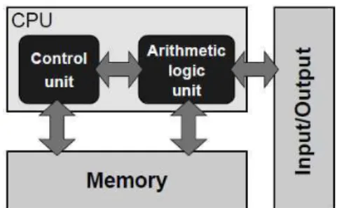
In Figure 2 we presented the block diagram of a stored-program type of com-puter. Its main feature which makes it different from the previous models is that its instructions are numbers which are memorised as data in the memory. The in-structions are real and executed by the control unit; a separate arithmetic/logic unit which is responsible for real computing and deals with data stored in the memory, together with the instructions. I/O facilitates the communication with the users. The control unit and the arithmetic unit together with the interfaces corre-sponding to the memory and I/O form a central processing unit (CPU-Central Proc-essing Unit).
Figure 2. Stored-program computer architecture.
Figure 2 describes a design with an undivided memory which stores both the program and the data (“stored program”) and a processing unit which executes the instructions, operating on the data. Likewise, the programs are allowed to modify or to generate other programs because the instructions and data are in the same “deposit”. This allows us to have editors and compilers: the computer treats the program’s code as some data on which it can operate [4].
The stored program, which loads the control unit is stored in the memory to-gether with any data that the arithmetic unit requires.
a high level of language such as C or Fortran into instructions which can be memo-rised in the memory and then executed on the computer.
This project is the basis of all today’s computing systems and its inherent problems still prevail:
• The instructions and data must continuously “load” the control units and the arithmetical one, but the speed of the memory interface represents a limitation of the computing performance. This brake is often called von Neumann bottleneck.
The architectural optimizations and the programming techniques can attenuate the adverse effects of this constraint, but it must be clear that this one remains one of the most severe limiting factors.
• The architecture is inherently sequential, processing a single instruction with a single operator or a group of operators from the memory. In this sense the concept SISD (Single Instruction Single Data) was created. There are possibilities of modification and extension of this architecture in order to support “different types” of parallelism and the way such a parallel machine can be efficiently used.
Despite these shortcomings, no other architectural concept was found for the wide use in a similar way during the 70 years of electronic digital calculation [5].
5. Parallel computers
We talk about parallel computing every time a number of “computing ele-ments” (cores) solve a problem in a cooperant way. All the modern architectures of supercomputers depend in a large measure on the parallelism and the number of processors in supercomputers which is in a continuous increase. The medium number of processors multiplied 50 times in the last decade. Between 2004 and 2009, the occurrence of multicore chips has led to a dramatic increase of the num-ber of the basic typical cores [7].
A parallel computer with shared memory is a system in which the number of processors works on a space of physical addresses shared and common for all the processors. Although transparent for the programmer in what concerns the func-tionality, there are two varieties of shared memory systems which have perform-ance characteristics very different concerning the access to the main memory, thus: uniform memory access (UMA) systems in which the latency and the band-width are the same for all the processors and all the memory locations, also called symmetric multiprocessing (SMP-symmetric multiprocessing), and cache-coherent nonuniform memory access (ccNUMA) in which the memory is physically distrib-uted but logically it is common (shared) [4].
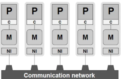
Figure 3 presents a simplified block diagram of a parallel computer with dis-tributed memory. Each P processor is connected to an exclusive local memory, meaning, no other CPU has direct access to it.
Figure 3. Simplified block diagram of a distributed memory parallel computer.
Nowadays, there is no distributed memory system. In this sense the scheme must be seen only as a programming model. Because of price/performance all the parallel machines of today, first of all the PC clusters are formed from a number of “computing nodes” with shared memory, with two or more processors; the point of view of distributed memory programmers does not reflect this. It is even possible (and rather usual) the use of programming the distributed memory on pure ma-chines with shared memory [5].
6. Applied development.
The optimization problem whose solution is sought to be accelerated using parallel computing is an electrostatic problem and it is described as follows: considered N electrons in a conducting body. The electrons arrange themselves to minimize their potential energy, subject to the constraint constraint of lying inside the conducting body. The electrons arrange themselves to minimize their potential energy subject to the constraint of lying inside the conducting body. At the minimum total potential energy, all the electrons lie on the boundary of the body. Because the electrons are indistinguishable, there is no unique minimum for this problem (permuting the electrons in one solution gives another valid solution).
The first phase of implementation of the above application, is the formulation of the problem in Matlab, therefore have made three Matlab files: electronProblemOptimization.m that implements the optimization problem, in Figure 4 is defined the objective function in sumInvDist.m file, and the nlConstraint.m file defines the non-linear constraints.
The optimization goal is to minimize the total potential energy of the electrons subject to the constraint that the electrons remain within the conducting body. The objective function, potential energy, is the sum of the inverses of the distances between each electron pair (i,j = 1, 2, 3,… E):
∑
<
−
=
ji
x
ix
jenergy
1
(1)
The objective function is defined in sumInvDist.m file, as follows:
The constraints that define the boundary of the conducting body are:
y
x
z
≤
−
−
(2)
( )
1
21
2
2
+
+
+
≤
z
y
x
(3)
The first inequality is a non-smooth nonlinear constraint because of the absolute values on x and y. Absolute values can be linearized to simplify the optimization problem. This constraint can be written in linear form as a set of four constraints for each electron, i, where the indices 1, 2, and 3 refer to the x, y, and z coordinates, respectively:
0
2 , 1 , 3,
−
i−
i≤
i
x
x
x
(4)
0
2 , 1 , 3,
−
i+
i≤
i
x
x
x
(5)
0
2 , 1 , 3,
+
i−
i≤
i
x
x
x
(6)
0
2 , 1 , 3,
+
i+
i≤
i
x
x
x
(7)
This problem can be solved with the nonlinear constrained solver fmincon in Optimization Toolbox. The fmincon solver (find minimum of constrained nonlinear multivariable function) trying to find a minimum of a constrained scalar function of several variables from an initial estimate. Generally this is called nonlinear constrained optimization (with difficulties) or nonlinear programming.
Linear inequality equations (Aineq*x = bineq) are defined for E electrons:
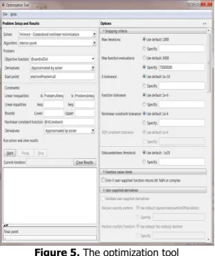
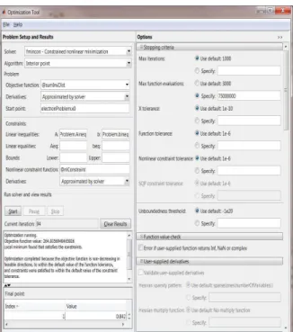
The execution upload the problem on the work space and opening of optimization tools shown in Figure 5:
Figure 5. The optimization tool
Figure 6. The oobjective function value and the number of iterations obtained from serial execution of optimization problems.
This provides a snapshot of electrons in the form of tears (as shown in Figure 7) and the elapsed time displayed in the command window.
Figure 7. Distribution of the electrons
Further, runs this optimization problem in parallel on four cores using parallel computing, opening an Matlab parallel session (matlabpool) that runs the specified optimization problem, as shown in the following sequence of code:
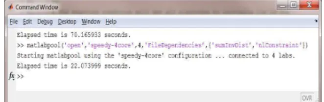
From Figure 8, which is a print screen of the commands window, we can see the value of the serial execution time for the optimization problem which is approximately equal to 70 seconds, and the parallel execution time achieved by the parallel execution of the optimization problem which is approximately equal to 22 seconds.
Figure 8. The result of serial and parallel execution (the serial and parallel time)
4. Conclusion
The obtained practical results confirms the theory on the utility of high performance scientific computing, taking into account the reduction of the execution time for optimization problem, which is an important performance aspect.
Using parallel computing to increase performance of solving the optimization problem formulated in this paper is just a simple example of when the parallel computing may prove useful, but surely that it is not unique, as mentioned in the first part of this paper where spoke about high performance computing and the possibilities of using it.
References
[2] Grama A., Gupta A., Karypis G., Kumar V., Introduction to Parallel Computing, 2nd edition, Addison-Wesley, 2003.
[3] Catanzaro B., Fox A.,. Keutzer K, Patterson D., Su Bor-Yiing, Snir M., Olukotun K., Hanrahan P., Chafi H., Ubiquitous Parallel Computing from Berkeley, Illinois, and Stanford, Micro, IEEE, vol.30, no.2, pp.41-55, March-April 2010.
[4] Hager G., Wellein G., Introduction to High Performance Computing for Scientists and Engineers, CRC Press Taylor & Francis Group, 2011.
[5] Levesque J., Wagenbreth G., High Performance Computing: Program-ming and Applications, Chapman and Hall/CRC, 2010.
[6] Michael T. Heath, Scientific Computing. An Intorductory Survey, The McGraw-Hill Companies, 2002.
[7] Victor Eijkhout, Edmond Chow, Robert van de Geijn, Introduction to High-Performance Scientific Computing, 2010.
Address: