Linear mixed-effects models to describe individual tree crown width for China-fir in Fujian Province, southeast China.

Linear Mixed-Effects Models to Describe

Individual Tree Crown Width for China-Fir in

Fujian Province, Southeast China

Xu Hao, Sun Yujun*, Wang Xinjie, Wang Jin, Fu Yao

Key Laboratory for Silviculture and Conservation of Ministry of Education, College of Forestry, Beijing Forestry University, Beijing, PR China

*sunyj@bjfu.edu.cn

Abstract

A multiple linear model was developed for individual tree crown width ofCunninghamia lan-ceolata(Lamb.) Hook in Fujian province, southeast China. Data were obtained from 55 sample plots of pure China-fir plantation stands. An Ordinary Linear Least Squares (OLS) regression was used to establish the crown width model. To adjust for correlations between observations from the same sample plots, we developed one level linear mixed-effects (LME) models based on the multiple linear model, which take into account the random ef-fects of plots. The best random efef-fects combinations for theLMEmodels were determined by the Akaike’s information criterion, the Bayesian information criterion and the -2logarithm likelihood. Heteroscedasticity was reduced by three residual variance functions: the power function, the exponential function and the constant plus power function. The spatial correla-tion was modeled by three correlacorrela-tion structures: the first-order autoregressive structure [AR(1)], a combination of first-order autoregressive and moving average structures [ARMA (1,1)], and the compound symmetry structure (CS). Then, theLMEmodel was compared to the multiple linear model using the absolute mean residual (AMR), the root mean square error (RMSE), and the adjusted coefficient of determination (adj-R2). For individual tree crown width models, the one levelLMEmodel showed the best performance. An indepen-dent dataset was used to test the performance of the models and to demonstrate the advan-tage of calibratingLMEmodels.

Introduction

China-fir (Cunninghamia lanceolata(Lamb.) Hook) is the most commonly grown afforesta-tion species in southeast China because of its fast growth and good wood qualities. It is widely used for buildings, furniture, bridge construction and many other purposes. According to the National Continuous Forest Inventory, approximately 11.26 million hectares and 734.09 mil-lion cubic meters of China-fir were distributed over 10 provinces in China in 2010.

OPEN ACCESS

Citation:Hao X, Yujun S, Xinjie W, Jin W, Yao F (2015) Linear Mixed-Effects Models to Describe Individual Tree Crown Width for China-Fir in Fujian Province, Southeast China. PLoS ONE 10(4): e0122257. doi:10.1371/journal.pone.0122257

Academic Editor:Rongling Wu, Pennsylvania State University, UNITED STATES

Received:November 7, 2014

Accepted:February 10, 2015

Published:April 15, 2015

Copyright:© 2015 Hao et al. This is an open access article distributed under the terms of theCreative Commons Attribution License, which permits unrestricted use, distribution, and reproduction in any medium, provided the original author and source are credited.

Data Availability Statement:All relevant data are within the paper.

Funding:This work was supported by the Special Public Interest Research and Industry Fund of Forestry (No.200904003-1) and the project of forestry science and technology research (No.2012-07). The funders had no role in study design, data collection and analysis, decision to publish, or preparation of the manuscript.

Growth and yield models are commonly used for forest management planning because they can simulate stand development and production under various management alternatives [1;2]. As an important tree variable, the crown width (CW) of individual trees is a fundamental com-ponent of forest growth and yield prediction frameworks [3;4], and it is also crucial for assess-ing the competitive level, tree vigor, microclimate, biological diversity, mechanical stability, fire susceptibility and behavior under wind stress, amongst other features [5]. The tree crown dis-plays the leaves to capture radiant energy for photosynthesis and is strongly correlated with tree growth [6]. Therefore, measurements of the tree crown are often made to aid the under-standing and quantification tree growth [7]. However, it is excessively costly and time consum-ing to measure the crown width of trees [8;9]. As a result, it is necessary to establish accurate crown width models for forest managers to predict crown width precisely based on the crown data from adequate numbers of sample trees within different sample plots.

Regression analysis, such as the Ordinary Linear least Squares (OLS) regression, is the most commonly used statistical method in forest modeling [10]. Most crown width models are sim-ple linear or nonlinear functions of diameter at breast height (DBH), estimated using linear or nonlinear regression [8;9]. The fitting data for crown width models are usually collected by measurements of trees within different plots, also known as cross-sectional data [11;12]. The hierarchical nature of the data results in spatial correlation among measurements made in the same sampling unit (i.e., plot) [13]. However, the hierarchical structure is often ignored and in-dependence of observations is assumed [8–10;14;15]. Furthermore, the data are autocorre-lated and cannot be considered independent samples of the basic plot population [13]. The OLSregression assumption of independent residuals is therefore violated, biasing the estimates of the standard error of the parameter estimates [16].

Linear mixed-effects (LME) models that include both fixed-effects and random-effects pro-vide an efficient means of analyzing some kinds of cross-sectional data [17;18]. The fixed-ef-fects parameters are associated with an entire population or with certain repeatable levels of experimental factors, and the random-effects parameters are related to individual experimental units drawn at random from a population. These parameters account for spatial correlation by defining the covariance structure of the model’s random component and by using this struc-ture during parameter estimation. Because of their advantages,LMEmodels provide an effi-cient statistical method for explicitly modeling hierarchical stochastic structure and are increasingly applied to forest growth and yield modeling [19–23]. Use ofLMEmodels allows the models to be calibrated by predicting random components from plot-level covariates when a new subject is available and is not used in the fitting of the model by using the empirical best linear unbiased predictors (EBLUPs) [22;24–26].

The main purpose of this research was to develop an individual tree crown width model for C.lanceolatain Fujian province, southeast China, on the basis of data derived from 55 sample plots. A one-level (plots effects) linear mixed modeling approach was applied to the hierarchi-cal structure of the data. This diminished the level of variance among the sampling units. Our preliminary analysis showed that theLMEmodel effectively removed the heteroscedasticity and spatial correlation in the data and therefore could be an important tool for the sustainable management of China-fir within the study area. The predictive ability of the developed model and the applicability of theLMEmodel were demonstrated using separate validation data.

Materials and Methods

Data

The pure China-fir stands are located in Jiangle County (117°050_-117°400_{E, 26°26}0_-27°040_N),

approximately 1699 mm, the annual mean frost-free season is 287 days, and the annual mean temperature is 18.7°C.

Data from four thousand one hundred ninety-nine trees were obtained from 55 single-spe-cies plots of plantation-grown China-fir on the Jiangle state-owned forest farm in Fujian Prov-ince, southeast China (Fig 1). The Jiangle state-owned forest farm issued permission for each location, and the field studies did not involve endangered or protected species. The sample plots were square and varied in size from 400 to 600 m2. All standing live trees (height>1.3 m) on

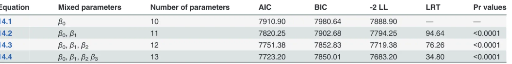
the plots were measured for DBH (outside bark), tree height, height to crown base (height above ground to crown base) and crown width. Three to five dominant trees on each plot were chosen to calculate plot dominant height and diameter. Crown width was taken as the arithmetic mean of two crown widths, obtained from measurements of four crown radii in four directions (from the east, west, south and north to the center of tree, respectively) representing two perpendicular azimuths [8]. The crown width data were randomly divided into two groups; 75% of the points were used for model fitting, and 25% were used for model validation, which can be claimed as independent. The fitting and validation data consisted of 2587 trees from 39 plots and 1613 trees from 16 plots, respectively. Summary statistics for both the fitting and validation data are shown inTable 1. The crown data are graphically depicted inFig 2.

Methods

The covariate selection. DBH is an important tree characteristic and the variable that has the greatest correlation with crown width [27]. In addition to DBH, CW is explained by other tree and stand attributes, [9;28] such as a reduction in growth from increases in stand density, SD (tree ha-1) and basal area, BA (m2ha-1) [22;29]. In addition, CW is also influence by tree size variables, such as sample tree height (H) and height to crown base (HCB), and stand vari-ables, such as stand age (A), plot dominant height, DH (m), plot dominant diameter at breast height, DD (cm), plot quadratic mean diameter, QMD (cm) [28;30;31], plot mean height, MH (m), and site index, SI (m at 20 yr).

Crown width multiple linear model. Independent variables were identified and a back-ward stepwise linear regression routine that started with all candidate variables, tested the dele-tion of each variable using a chosen model comparison criterion, deleted the variable (if any) whose removal improved the model the most, and repeated this process until no further im-provement was possible, was applied to reduce the number of chosen variables to avoid

Fig 1. Fifty-five sample plots of pure China-fir plantation stands.

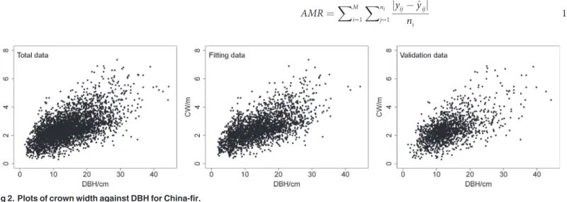
overfitting. Variance inflation factors (VIF<10), which provide an index that measures how much the variance of an estimated regression coefficient is increased because of collinearity, were also computed to reduce the number of chosen variables to avoid multicollinearity, which could result in numerically unstable estimates of the regression coefficients. Stepwise regression fits an observed dependent dataset using a linear combination of independent variables. The statistical methods were implemented in R, which is a free software environment for statistical computing and graphics [32]. The dependent variable is determined from a linear equation combining the values of the independent dataset with coefficients established by the regression. The statistical results were assessed in terms of the absolute mean residual (AMR), root mean square error (RMSE), and the adjusted coefficient of determination (adj-R2), which accounts for the number of predictors. The calculation formulas of these statistics are listed as follows:

AMR¼XM i¼1

Xni

j¼1

jyij y^ijj

ni

1

Table 1. Summary statistics for increments datasets.

Variables Fitting data Validation data

Mean Min Max sd Mean Min Max sd

CW (m) 2.53 0.4 7.4 0.95 2.42 0.3 8.2 0.93

DBH (cm) 14.44 2.0 44.4 6.75 13.54 1.5 44.2 5.84

H(m) 13.36 1.2 36.5 5.56 12.11 1.3 30.8 5.35

HCB (m) 7.68 0.1 21.5 4.08 6.98 0.3 19.8 4.52

DH (m) 18.01 6.9 30.3 4.93 15.78 6.5 26.2 5.78

DD (cm) 21.43 8.0 38.6 5.13 20.43 10.1 36.0 6.88

A(yr) 22.63 7.0 49.0 9.43 18.10 5.0 40.0 8.73

SI (m at 20 years) 17.13 12.0 24.0 3.69 16.89 12.0 22.0 2.86

SD (trees ha-1) 2311 617 4500 1044.85 2862 467 4400 907.91

QMD (cm) 15.03 4.8 25.2 4.64 13.80 9.9 26.9 3.50

MH (m) 14.01 4.2 21.3 4.00 12.06 5.0 21.4 4.25

BA (m2_ha-1_{). 29.54 3.4 68.0 16.11 42.4 16.9 99.82 20.11}

doi:10.1371/journal.pone.0122257.t001

Fig 2. Plots of crown width against DBH for China-fir.

RMSE¼

ffiffiffiffiffiffiffiffiffiffiffiffiffiffiffiffiffiffiffiffiffiffiffiffiffiffiffiffiffiffiffiffiffiffiffiffiffiffiffiffiffiffiffiffi XM

i¼1

Xni

j¼1

ðyij ^yijÞ

2

ni r s

2

adj R2_{¼1 ðn}

ij 1Þ XM

i¼1

Xni

j¼1

ðyij ^yijÞ

2

ni r XM

i¼1

Xni

j¼1ðyij

yÞ2

2

6 6 6 4

3

7 7 7 5

3

whereMis the number of plots,niis the number of observations in ploti,ris the number of

parameters in the model,yijis the crown width of thejth tree taken from theith plot,ŷijis the

crown width prediction, and_{yis the average of observations. The accuracy of the models was}

tested against thefitting data and against independent validation data from the same plot [23]. LME_{model method. Available data were from measurements of trees located in sample} plots. Because of this nested structure, there is high correlation among observations taken from the same plot. To alleviate this issue, a linear mixed-effects model approach has been proposed by other authors [10;33]. For a single level of grouping, a general expression for aLMEmodel can be defined as [17;20;34]:

CWij¼XijbþZijbijþεij; i¼1; :::;M ; j¼1; :::;ni

bijNð0;DÞ; εijNð0;RijÞ

4

where CWijis the crown width of thejth tree taken from theith plot,βis thep-dimensional

vector offixed effects (wherepis the number offixed-effects parameters in the model),bijis

theq-dimensional vector of random effects associated with plotithat is assumed to follow a normal distribution with mean zero and a variance-covariance matrixD(whereqis the num-ber of random-effects parameters in the model),Xij(of sizeni×p) andZi(of sizeni×q) are

knownfixed-effects and random-effects regressor matrices, and_ijis then_i-dimensional

with-in-group error vector with a spherical Gaussian distribution [35], which is assumed to be nor-mally distributed with zero expectation and a positive-definite variance-covariance structure Rij, generally is ani× 1 vector for the residual items [ei1,ei2,ei3,. . .,eij,. . .,eini]

T_{[36]. Both the}

random-effectsbijand the within-group errorsijare assumed to be independent for different

groups and to be independent of each other for the same group.

Ascertainment of mixed parameters. To fit the mixed-effects models, the key question is which parameters in the model should be considered as random effects and which ones could be treated as purely fixed effects. Generally, an alternative model-building approach is to start with a model with random effects for all parameters and then examine the fitted object to de-cide which, if any, of the random effects can be eliminated from the model [18]. Therefore, dif-ferent combinations of model parameters were tested to ascertain their importance with respect to crown width, and the best model was selected by Akaike’s information criterion (AIC) [37], Bayesian information criterion (BIC) [38] and -2 logarithm likelihood (-2 LL) [31]. The less criteria a model has, the better it performs. An appropriate variance function structure forLMEmodels were determined by a likelihood ratio test (LRT) [18;39]. AllLMEmodels presented in this paper were fitted using theLMEfunction in the R statistical

software environment.

heteroscedasticity and spatial correlation [35;36;40]. A general expression for the matrix is given by [40;41]:

R¼s2 G0:5

IG0:5

5

where (in this case) for treejin ploti, withniincrement,Ris theni×niintraindividual

variance-covariance matrix which defines within-group variability,Gis ani×nidiagonal matrix of the

within-group error variance structure (heteroscedasticity),Iis ani×nimatrix showing the

with-in-group autocorrelation structure of error, andσ2is a scaling factor for the error dispersion

[10]. To remove variance heterogeneity, we used the power function, exponential function and constant plus power function as the variance functions tofit crown width models [18].

Vðε

ijÞ ¼s

2 DBH2d

ij 6

Vðε

ijÞ ¼s

2

expð2_dDBH

ijÞ 7

Vðε

ijÞ ¼s

2

ðd1þDBHd2

ijÞ

2

8

Correlation structures were used to address the within-tree spatial correlations observed in the data [42;43]. A method was selected from among three commonly used approaches: the first-order autoregressive structure [AR(1)], a combination offirst-order autoregressive and moving average structures [ARMA(1,1)], and the compound symmetry structure (CS) [18].

ARð1_{Þ ¼s}2

1 _{r r}2

r 1 _r

r2 r 1 2 6 4 3 7 5 9

ARMAð1_; 1_{Þ ¼s}2

1 _{g gr}

g 1 _g

gr g 1 2 6 4 3 7 5 10 CS¼ s2

þs1 s1 s1

s1 s2

þs1 s1

s1 s1 s2

þs1 2 6 4 3 7 5 11

whereρis the autoregressive parameter,γis a moving average component, andσ₁is the

residu-al covariance [44;45].

Parameter estimation. The parameters in the equations were estimated by maximum likelihood (ML) using the Lindstrom and Bates (LB) algorithm implemented in the RLME function [17;18]. The LB algorithm andLMEfunction are detailed in several articles; see, for example, [17;18].

A key question in fitting theLMEmodels is to estimate the random effects parameters. In this study, they can be calculated with the information from measured trees, such as the mea-surements of CW and DBH, by the Empirical Best Linear Unbiased Predictors (EBLUPs) [34].

^

bijk ^

DZ^TðR^þZ^D^Z^TÞ 1^ε

ijk 12

whereD^ is the estimated variance-covariance matrix for the random-effectsb^ijk, ^

estimated variance-covariance matrix for the error term, andZ^is the estimated partial deriva-tives matrix with respect to random effects parameters.

Results

Selection of the basic crown width model

The following formula is the composition of individual tree size variables and stand variables for predicting crown width usingOLS:

CWij¼b0þb1DBHijþb2Hijþb3HCBijþb4DHiþb5DDiþb6Ai

þb7SIiþb8SDiþb9QMDiþb10MHiþb11BAiþεij

13

whereβ₀-β₁₁are the formal parameters.

To avoid overfitting and multicollinearity between independent variables, the backward stepwise linear regression routine and the variance inflation factor were used to reduce the number of chosen variables. In addition, we took into account the biologically reasonable and the factors that exhibited significance (Pr value<0.05) between independent variables. The var-iable selection process involves a series of steps beginning with the stepwise regression method together with VIF control to identify those variables that may be useful in the model. DH,A and MH were removed fromEq 13because their VIF>10 (VIFDH= 27.48, VIFA= 13.61,

VIFMH= 17.72). As a result, the final diameter growth model for fir plantations can be

express-ed as:

CWij¼b0þb1DBHijþb2Hijþb3HCBijþb4DDiþb5SIiþb6SDiþb7QMDiþb8BAiþεij 14

The statistics used for the selection of the basic model are shown with equations inTable 2.

Construction of

LME

models

There would be ninety different combinations of no more than four random-effects parameters forEq 14while simultaneously considering plots effects. TheLMEmodels with more than four random-effects parameters could not reach convergence.

LRT, AIC, BIC and -2 LL statistics were compared between theLMEmodels with the best dif-ferent combinations of random-effects parameters and are shown inTable 3. The model ofEq 14, incorporating plots effects onβ0,β1,β2andβ3(Eq 14.4), yielded the smallest AIC, BIC and -2 LL

(Pr<0.0001).

CWij¼ ðb0þu0iÞ þb1DBHijþb2Hijþb3HCBij

þb4DDiþb5SIiþb6SDiþb7QMDiþb8BAiþεij

14:1

CWij¼ ðb0þu0iÞ þ ðb1þu1iÞDBHijþb2Hijþb3HCBij

þb4DDiþb5SIiþb6SDiþb7QMDiþb8BAiþεij

14:2

CWij¼ ðb0þu0iÞ þ ðb1þu1iÞDBHijþ ðb2þu2iÞHijþb3HCBij

þb4DDiþb5SIiþb6SDiþb7QMDiþb8BAiþεij

14:3

CWij¼ ðb0þu0iÞ þ ðb1þu1iÞDBHijþ ðb2þu2iÞHijþ ðb3þu3iÞHCBij

þb4DD_iþb5SI_iþb6SD_iþb7QMD_iþb8BA_iþε

ij

14:4

whereβ0-β8are thefixed effects parameters andu0i,u1i,u2iandu3iare the random-effects

pa-rameters generated by plots effects onβ₀,β₁,β₂andβ₃, respectively.

LME

model with heteroscedasticity and spatial correlation

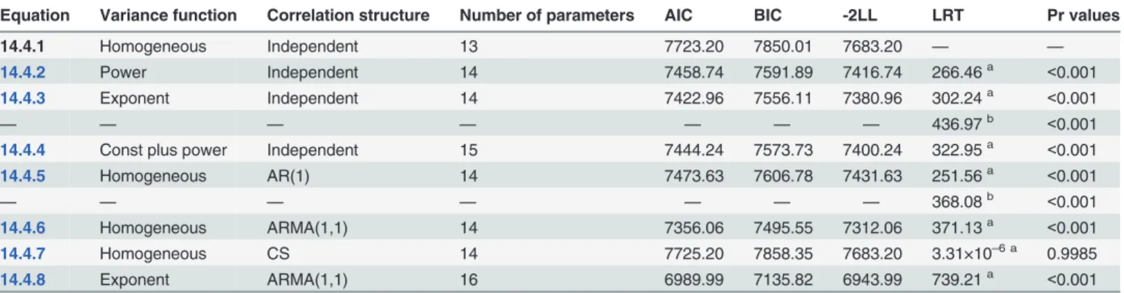
We used the power function, the exponential function or the constant plus power function as the variance functions and AR, ARMA(1,1) or CS as the correlation structure to update Eq 14.4to reduce heteroscedasticity and spatial correlation. TheLMEmodels with variance functions and correlation structures are shown inTable 4. In this study, Equation 14.4.1 is the same asEq 14. The best models were chosen with the smallest AIC, BIC and -2 LL. Thus, the

Table 2. Comparison of fitting statistics and estimated variance components of the models with different alternatives of covariates inclusion, re-sidual variance function and variance components estimation method.

Model Intercept DBH H HCB DD SI SD QMD BA

Eq 14 1.3450 0.1235 -0.0212 -0.0275 0.0236 -0.0077 2.31×10–5 -0.0127 -0.0105

(standard error) (0.0904***) (0.0032***) (0.0050***) (0.0045***) (0.0035***) (0.0037*) (4.4×10–5*) (0.0054**) (0.0009***)

Eq 14.4 1.1812 0.1103 0.0073 -0.0238 0.0152 -0.0115 9.07×10–5 -0.0182 -0.0060

(standard error) (0.5102) (0.0066**) (0.0080*) (0.0079) (0.0193) (0.0197) (7.68×10–5**) (0.0265) (0.0048)

Eq 14.4.8 0.6693 0.1090 0.0085 -0.0217 0.0231 -0.0134 0.0002 -6.93×10–3 -0.0075

(standard error) (0.4490*) (0.0061***) (0.0060*) (0.0062**) (0.0154*) (0.0163*) (0.0001**) (0.0217*) (0.0038**)

“*”means Pr value<0.05 “**”means Pr value<_0.01

“***”means Pr values<0.001.

doi:10.1371/journal.pone.0122257.t002

Table 3. Performance criteria ofLMEmodels for combinations of random effects.

Equation Mixed parameters Number of parameters AIC BIC -2 LL LRT Pr values

14.1 β0 10 7910.90 7980.64 7888.90 — —

14.2 β0,β1 11 7820.25 7902.68 7794.25 94.64 <0.0001

14.3 β0,β1,β2 12 7751.38 7852.83 7719.38 76.26 <0.0001

14.4 β0,β1,β2β3 13 7723.20 7850.01 7683.20 34.80 <0.0001

final models of plots effects are:

Equation14_:4_þEquation6 _14:4:2

Equation14_:4_þEquation7 _14:4:3

Equation14_:4_þEquation8 _14:4:4

Equation14_:4_þEquation9 _14:4:5

Equation14_:4_þEquation10 _14:4:6

Equation14_:4_þEquation11 _14:4:7

Equation14_:4_þEquation6_þEquation10 _14:4:8

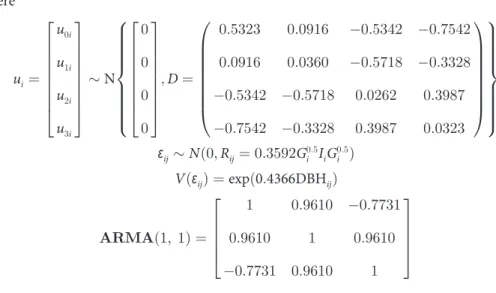
Parameter estimates

TheLMECW model with plots effects is then defined by the following expression:

CWij¼ ð0:8247þu0iÞ þ ð0:1093þu1iÞDBHijþ ð0:0095þu2iÞHijþ ð 0:0219þu3iÞHCBij

þ0_:0181_DD

i 0:0105SIiþ0:0004SDi 0:0121QMDi 0:0064BAiþεij

15

Table 4. Comparisons of intercept effect mixed model performance for fir plantations diameter increment data with different within-tree correlation structures and different variance functions.

Equation Variance function Correlation structure Number of parameters AIC BIC -2LL LRT Pr values

14.4.1 Homogeneous Independent 13 7723.20 7850.01 7683.20 — —

14.4.2 Power Independent 14 7458.74 7591.89 7416.74 266.46a <_0.001

14.4.3 Exponent Independent 14 7422.96 7556.11 7380.96 302.24a _<0.001

— — — — — — — 436.97b _<0.001

14.4.4 Const plus power Independent 15 7444.24 7573.73 7400.24 322.95a _<0.001

14.4.5 Homogeneous AR(1) 14 7473.63 7606.78 7431.63 251.56a <_0.001

— — — — — — — 368.08b _<0.001

14.4.6 Homogeneous ARMA(1,1) 14 7356.06 7495.55 7312.06 371.13a _<0.001

14.4.7 Homogeneous CS 14 7725.20 7858.35 7683.20 3.31×10–6 a _0.9985

14.4.8 Exponent ARMA(1,1) 16 6989.99 7135.82 6943.99 739.21a <_0.001

a_{Likelihood ratio is calculated with respect to Equation 14.4.1} b

Likelihood ratio is calculated with respect toEq 14.4.8

Where

ui ¼

u0i u1i u2i u3i 2 6 6 6 6 6 6 6 4 3 7 7 7 7 7 7 7 5 N 0 0 0 0 2 6 6 6 6 6 6 6 4 3 7 7 7 7 7 7 7 5

;D¼

0_:5323 0_:0916 0_:5342 0_:7542

0_:0916 0_:0360 0_:5718 0_:3328

0_:5342 0_:5718 0_:0262 0_:3987

0_:7542 0_:3328 0_:3987 0_:0323 0 B B B B B B B @ 1 C C C C C C C A 8 > > > > > > > < > > > > > > > : 9 > > > > > > > = > > > > > > > ; ε

ijNð0;Rij¼0:3592G

0_:5

i IiG

0_:5

i Þ

Vðε

ijÞ ¼expð0:4366DBHijÞ

ARMAð1_; 1_{Þ ¼}

1 0_:9610 0_:7731

0_:9610 1 0_:9610

0_:7731 0_:9610 1 2 6 6 6 4 3 7 7 7 5

Model prediction

The predictive ability ofEq 14was evaluated using prediction procedures andEq 1–3on both fitting and validation data. The performance of theLMEmodels, with and without modeling the error structure, was evaluated using cross-validation procedures for both fitting and valida-tion data; the random effects were predicted with the EBLUPs (Eq 12), using the

measurement data.

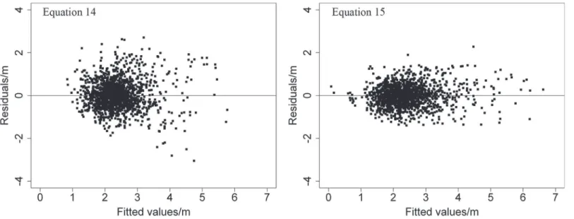
Table 5lists the three prediction statistics ofEq 14,Eq 15andEq 15without random effects for both fitting and validation data. Compared withEq 14,Eq 15had a higher adj-R2, 0.7226 compared to 0.4733, and lowerRMSE, 0.4854 compared to 0.6688, andAMR, 0.3688 compared 0.4954, for the validation data. InFig 3, the residuals of Eq14and15are plotted against the fit-ted values. The fitfit-ted values of these equations are plotfit-ted against the observed values inFig 4. Based on the above analysis, we can conclude thatEq 15, incorporating the random effects plots, was better thanEq 14. TheLMEmodel provides a model for predicting the expected val-ues of crown width for individual trees of China-fir in the single-species plantations of the study area.

Discussion

In this study, a backward stepwise linear regression was used to establish a multiple linear indi-vidual tree crown width model for China-fir. The relative importance of explanatory variables used to predict the crown width were assessed. Generally, DBH is the tree size variable most re-lated to crown width [27]. In addition to DBH, the tree size variables (such as H and HCB in this study) and stand variables (such as DH in this study) are also obvious factors affecting the crown width [20;22;46;47]. Both stand and tree development are linked to the DH because it

Table 5. Evaluation indices of each model.

Model Effects Fitting data Validation data

AMR RMSE adj-R2 _{AMR RMSE adj-R}2

Eq 14 0.5306 0.6914 0.4694 0.4954 0.6688 0.4733

Eq 15 Mixed effects 0.4027 0.5070 0.7147 0.3688 0.4854 0.7226

is a measureable stand characteristic that indicates site quality in terms of the stand growth and yield capacity [20]. The variables H and HCB showed a significant effect on the crown width because they are closely related to tree size and have an important role in crown fire initiation and spread [47;48]. Therefore, we selected the diameter at breast height, tree height, height to crown base, plot dominant height, plot dominant diameter at breast height, stand age, site index, stand density, plot quadratic mean diameter, plot mean height and basal area as the dependent variables to establish an individual tree crown width model. However, variance in-flation factors were used to avoid potential overfitting and multicollinearity.

Fig 3. Distribution of residuals for two equations fitting crown width of China-fir trees.

doi:10.1371/journal.pone.0122257.g003

Fig 4. Fitted values of two equations for crown width of China-fir trees against observed values.

Conclusions

Eleven variables were selected in this study to describe crown width (Eq 13) of China-fir in pure plantation stands in Fujian province, southeast China. Then, the backward stepwise linear regression routine and the variance inflation factor were used to reduce the number of chosen variables (Eq 14). The one-level (plot)LMEmodel using the variance function structure and correlation structure approach were used to estimate the relationship of the chosen variables with crown width for individual trees. The results showed that the one-levelLMEmodels with mixed effects, considering variance function structure and correlation structure (Eq 15), pro-vided better model fitting and more precise estimations than theLMEmodels without mixed effects (Eq 14) (Table 5and Figs3and4). Therefore, we recommend using a linear mixed ef-fects modeling approach to build an individual tree crown width model.

Author Contributions

Conceived and designed the experiments: XH SYJ. Performed the experiments: XH SYJ WXJ WJ FY. Analyzed the data: XH WJ FY. Contributed reagents/materials/analysis tools: XH SYJ WXJ WJ FY. Wrote the paper: XH.

References

1. Leites LP, Robinson AP, Crookston NL (2009) Accuracy and equivalence testing of crown ratio models and assessment of their impact on diameter growth and basal area increment predictions of two vari-ants of the Forest Vegetation Simulator. Can J Forest Res 39:3.

2. Canavan SJ, Ramm CW (2000) Accuracy and Precision of 10 Year Predictions for Forest Vegetation Simulator—Lake States. Northern Journal of Applied Forestry 17:2.

3. Tahvanainen T, Forss E (2008) Individual tree models for the crown biomass distribution of Scots pine, Norway spruce and birch in Finland. Forest Ecol Manag 255:3.

4. Peper PJ, McPherson EG, Mori SM (2001) Equations for predicting diameter, height, crown width, and leaf area of San Joaquin Valley street trees. Journal of Arboriculture 27:6.

5. Crecente-Campo F, Alvarez Gonzalez JG, Castedo-Dorado F, Gomez-Garcia E, Dieguez-Aranda U (2013) Development of crown profile models forPinus pinasterAit. andPinus sylvestrisL. in northwest-ern Spain. Forestry 86:4.

6. Dutilleul P, Herman M, Avella-Shaw T (1998) Growth rate effects on correlations among ring width, wood density, and mean tracheid length in Norway spruce (Picea abies). Can J Forest Res 28:1.

7. Kjelgren RK, Clark JR (1992) Photosynthesis and leaf morphology ofLiquidambar styracifluaL. under variable urban radiant-energy conditions. Int J Biometeorol 36:3.

8. Bragg DC (2001) A local basal area adjustment for crown width prediction. Northern Journal of Applied Forestry 18:1.

9. Sönmez T (2009) Diameter at breast height-crown diameter prediction models forPicea orientalis. Afri-can Journal of Agricultural Research 4:3.

10. Grégoire TG, Schabenberger O, Barrett JP (1995) Linear modelling of irregularly spaced, unbalanced, longitudinal data from permanent-plot measurements. Can J Forest Res 1:25.

11. Peugh JL, Enders CK (2005) Using the SPSS mixed procedure to fit cross-sectional and longitudinal multilevel models. Educ Psychol Meas 65:5.

12. Waring RH, Schroeder PE, Oren R (1982) Application of the pipe model theory to predict canopy leaf area. Can J Forest Res 12:3.

13. Fox JC, Ades PK, Bi H (2001) Stochastic structure and individual-tree growth models. Forest Ecol Manag 154:1.

14. Biging GS (1985) Improved estimates of site index curves using a varying-parameter mode. Forest Sci 31:1.

15. Keselman HJ, Algina J, Kowalchuk RK, Wolfinger RD (1999) A comparison of recent approaches to the analysis of repeated measurements. British Journal of Mathematical and Statistical Psychology: 52. PMID:10613111

17. Lindstrom MJ, Bates DM (1990) Nonlinear mixed effects models for repeated measures data. Bio-metrics 46.

18. Pinheiro JC, Bates DM (2000) Mixed Effects Models in S and S-Plus. New York: 291–342 p.

19. Matos LA, Lachos VH, Balakrishnan N, Labra FV (2012) Influence diagnostics in linear and nonlinear mixed-effects models with censored data. Comput Stat Data An 57:1.

20. Fu L, Sun H, Sharma RP, Lei Y, Zhang H, Tang S (2013) Nonlinear mixed-effects crown width models for individual trees of Chinese fir (Cunninghamia lanceolata) in south-central China. Forest Ecol Manag 302.

21. Timilsina N, Staudhammer CL (2013) Individual Tree-Based Diameter Growth Model of Slash Pine in Florida Using Nonlinear Mixed Modeling. Forest Sci 59:1.

22. Lhotka JM, Loewenstein EF (2011) An individual-tree diameter growth model for managed uneven-aged oak-shortleaf pine stands in the Ozark Highlands of Missouri, USA. Forest Ecol Manag 261:3.

23. Adame P, Hynynen J, Canellas I, Del Rio M (2008) Individual-tree diameter growth model for rebollo oak (Quercus pyrenaicaWilld.) coppices. Forest Ecol Manag 255:3–4.

24. Nigh G (2012) Calculating empirical best linear unbiased predictors (EBLUPs) for nonlinear mixed ef-fects models in Excel/Solver. Forest Chron 88:3. doi:doi:10.2223/JPED.2181PMID:22491787

25. Adame P, Del Rio M, Canellas I (2008) A mixed nonlinear height-diameter model for pyrenean oak (Quercus pyrenaicaWilld.). Forest Ecol Manag 256:1–2.

26. Calama R, Montero G (2005) Multilevel linear mixed model for tree diameter increment in stone pine (Pinus pinea): a calibrating approach. Silva Fenn 39:1.

27. Warbington R, Levitan J (1993) How to estimate canopy over using maximum crown width/DBH rela-tionships, Stand Inventory Technologies '92, Portland, pp. 319–328.

28. Uzoh FCC, Oliver WW (2008) Individual tree diameter increment model for managed even-aged stands of ponderosa pine throughout the western United States using a multilevel linear mixed effects model. Forest Ecol Manag 256:3.

29. Wykoff WR (1990) A basal area increment model for individual conifers in the northern Rocky Moun-tains. Forest Sci 36:4.

30. Adame P, Ca N Ellas I, Roig S, Del R I O M (2006) Modelling dominant height growth and site index curves for rebollo oak (Quercus pyrenaicaWilld.). Ann Forest Sci 63:8.

31. Zhao L, Li C, Tang S (2012) Individual-tree diameter growth model for fir plantations based on multi-level linear mixed effects models across southeast China. Journal of Forest Research 18:4.

32. Ihaka R, Gentleman R (2004) R: a language and environment for statistical computing, R Foundation for Statistical Computing, Vienna, Austria.

33. Palmer MJ, Phillips BF, Smith GT (1991) Application of nonlinear models with random coefficients to growth data. Biometrics 47.

34. Vonesh E, Chinchilli VM (1997) Linear and nonlinear models for the analysis of repeated measure-ments. New York: 61–84 p.

35. Davidian M, Giltinan DM (1995) Nonlinear models for repeated measurement data. New York: 58–74 p.

36. Meng SX, Huang S (2009) Improved calibration of nonlinear mixed-effects models demonstrated on a height growth function. Forest Sci 55:3.

37. Akaike H (1974) A new look at the statistical model identification. Automatic Control, IEEE Transactions on 19:6.

38. Weiss RE (2005) Modeling longitudinal data. New York: 19–21 p.

39. Fang Z, Bailey RL (2001) Nonlinear mixed effects modeling for slash pine dominant height growth fol-lowing intensive silvicultural treatments. Forest Sci 47:3.

40. Calama R, Montero G (2004) Interregional nonlinear height-diameter model with random coefficients for stone pine in Spain. Can J Forest Res 34:1.

41. Crecente-Campo F, Tome M, Soares P, Dieguez-Aranda U (2010) A generalized nonlinear mixed-ef-fects height-diameter model forEucalyptus globulusL. in northwestern Spain. Forest Ecol Manag 259:5.

42. Lappi J, Malinen J (1994) Random parameter height-age models when stand parameters and stand age are correlated. Forest Sci 40:4.

43. Omule SAY, MacDonald RN (1991) Simultaneous curve fitting for repeated height-diameter measure-ments. Can J Forest Res 21:9.

44. Leak W (1996) Analysis of multiple systematic remeasurement. Forest Sci 1:12.

46. Gonzalez-Benecke CA, Gezan SA, Samuelson LJ, Cropper WP Jr, Leduc DJ, et al. (2014) Estimating

Pinus palustristree diameter and stem volume from tree height, crown area and stand-level parame-ters. Journal of Forestry Research 25:1.

47. Gómez-Vázquez I, Fernandes PM, Arias-Rodil M, Barrio-Anta M, Castedo-Dorado F (2013) Using den-sity management diagrams to assess crown fire potential inPinus pinasterAit. stands. Ann Forest Sci.