www.nonlin-processes-geophys.net/21/187/2014/ doi:10.5194/npg-21-187-2014
© Author(s) 2014. CC Attribution 3.0 License.
Nonlinear Processes
in Geophysics
Diagnostics on the cost-function in variational assimilations for
meteorological models
Y. Michel
Météo-France and CNRS, CNRM-GAME, UMR3589, Toulouse, France Correspondence to:Y. Michel ([email protected])
Received: 10 July 2013 – Revised: 5 December 2013 – Accepted: 5 December 2013 – Published: 5 February 2014
Abstract. Several consistency diagnostics have been pro-posed to evaluate variational assimilation schemes. The “Bennett-Talagrand” criterion in particular shows that the cost-function at the minimum should be close to half the number of assimilated observations when statistics are cor-rectly specified. It has been further shown that sub-parts of the cost function also had statistical expectations that could be expressed as traces of large matrices, and that this could be exploited for variance tuning and hypothesis testing.
The aim of this work is to extend those results using stan-dard theory of quadratic forms in random variables. The first step is to express the sub-parts of the cost function as quadratic forms in the innovation vector. Then, it is possi-ble to derive expressions for the statistical expectations, vari-ances and cross-covarivari-ances (whether the statistics are cor-rectly specified or not). As a consequence it is proven in par-ticular that, in a perfect system, the values of the background and observation parts of the cost function at the minimum are positively correlated. These results are illustrated in a simpli-fied variational scheme in a one-dimensional context.
These expressions involve the computation of the trace of large matrices that are generally unavailable in variational formulations of the assimilation problem. It is shown that the randomization algorithm proposed in the literature can be ex-tended to cover these computations, yet at the price of addi-tional minimizations. This is shown to provide estimations of background and observation errors that improve forecasts of the operational ARPEGE model.
1 Introduction
Most operational data assimilation schemes in meteorol-ogy are loosely based on statistical linear estimation (e.g. Talagrand, 2010. The variational formulation (Le Dimet and
Talagrand, 1986; Courtier et al., 1998; Rabier et al., 2000) has proven very effective in assimilating directly and mas-sively satellite observations, which has been a source of huge progress in numerical weather prediction (Simmons and Hollingsworth, 2002; Rabier, 2005). The cost function to be minimized measures the distances of the atmospheric state to the observations and to the background, weighted by the inverse of their error covariances. These error statis-tics are unfortunately not very well known. Common meth-ods to estimate observation errors include the innovation ap-proach (Hollingsworth and Lonnberg, 1986; Daley, 1993), where observation error statistics are taken to be spatially uncorrelated and are deduced from the innovation covari-ance. Background error statistics are estimated within an existing data assimilation scheme, for instance using fore-casts at different ranges valid at the same time (Parrish and Derber, 1992; Derber and Bouttier, 1999) or, more re-cently and inspired by the Ensemble Kalman Filter (e.g. Evensen, 2003), ensembles of perturbed variational assimi-lations (Fisher, 2003; Kucukkaraca and Fisher, 2006; Belo-Pereira and Berre, 2006).
Despite this recent progress, it is still necessary and useful to check for the consistency between the prescribed statistics and the a posteriori error statistics. Any inconsistency could help to point out imperfections in the specification of the statistics. Objective assessment of the quality of assimilation schemes can only be performed against independent observa-tions that are not used in the estimation process (Talagrand, 1999). Yet internal consistency diagnostics can also prove useful. Two applications of these kinds of diagnostics have been proposed: hypothesis testing (Muccino et al., 2004) and variance tuning (Desroziers and Ivanov, 2001; Chapnik et al., 2006).
the errors in the innovation vector. In the perfect case, the minimum value of the cost function has a χp2 distribution wherepis the number of scalar observations assimilated in the system (Bennett et al., 1993; Talagrand, 1999). However, the values of the cost function were found to differ signif-icantly from their expectation in a series of data assimila-tion experiments with an ocean model (Bennett et al., 2000). Muccino et al. (2004) also studied how various errors in the specified error covariance matrices were affecting the distri-bution of the value of the cost function at the minimum. A Kolmogorov–Smirnov test was used to identify departures from theχ2distribution, with significant skill in some cases. When certain sets of observations are taken to have un-correlated errors, it is possible to split the observation term further as the sum of sub-functions. The expectation of these sub-functions can still be expressed (Talagrand, 1999) as the trace of large matrices. Desroziers and Ivanov (2001) (here-after DI01) proposed to estimate these traces using a ran-domization algorithm. They also proposed an iterative ap-proach for tuning the variances. It enforces consistency be-tween the observed value of the sub-parts of the cost func-tions and their theoretical expectafunc-tions as computed by the randomized trace estimation. This method was later shown (Chapnik et al., 2004) to be similar to a maximum-likelihood approach. Operational implementation of the scheme in the global model ARPEGE1 from Météo-France was achieved by Chapnik et al. (2006), and the tuning of observation er-ror variances yielded a positive impact on both analyses and forecasts. The implementation in a limited area model was discussed by Sadiki and Fischer (2005). They proposed in particular the use of time or space averages to improve sam-pling. Finally, the ensemble of variational assimilations with perturbed observations as implemented at Météo-France and ECMWF (Kucukkaraca and Fisher, 2006) typically uses as-similations with perturbed backgrounds and observations. Desroziers et al. (2009) then showed that the previous sta-tistical expressions were a direct by-product of such an en-semble.
More precisely, Dee (1995) and Dee and da Silva (1999) have introduced the maximum-likelihood approach for the estimation of covariance parameters in meteorology. The likelihood function to be optimized with respect to these co-variance parameters is the sum of a quadratic form in the innovation vector and the log-determinant of a precision (in-verse covariance) matrix. Because of the very large size of the innovation vector (currently of the order of 106elements in the ARPEGE 4D-Var), a direct computation (using for in-stance Choleski decomposition) is not feasible. The approach that was favored in meteorology is to evaluate the deriva-tives (rather than the absolute values) of the likelihood func-tion and then using stochastic trace estimafunc-tion techniques, as demonstrated by Purser and Parrish (2003) in an ideal-1“Action de Recherche Petite Echelle Grande Echelle”, see
Pailleux et al., 2000 for a historical description
ized context. This stochastic approximation is nearly opti-mal in a well-define sense as proven by Stein et al. (2013). It is also possible that direct evaluation of the log-likelihood may become feasible even in high dimensions as shown by Aune et al. (2012). This required in particular (i) more ef-ficient evaluation of the trace with probing vectors (Bekas et al., 2007) and (ii) Krylov subspace methods for matrix in-versions (Saad, 2003). These approaches look very promis-ing, but as recognized by Purser and Parrish (2003), it is still necessary to experiment with various aspects in mete-orology including non-linear observation operators and in-troduction of a prior term (to stabilize the solution when the number of estimated parameters become large). This study rather builds upon the simpler but convenient approach taken in DI01 for variance tuning. However, it should be stressed that this approach is unlikely to be easily extended to the esti-mation of other paramaters such as localisation lengthscales (Houtekamer and Mitchell, 2001), or to the heteromorphic case where there is a need to compare log-likelihoods asso-ciated with covariances that use completely different sets of parameters (Purser and Parrish, 2003).
The aim of this paper is to present a different way of deriv-ing the Bennett-Talagrand criterion. The sub-parts of the cost function at the minimum are expressed as quadratic forms in the innovation vector. This allows the application of the the-ory of quadratic forms in random variables as summarized in Mathai and Provost (1992) (hereafter M92). The statistical expectation, variances and cross-covariances between sub-parts of the cost-function at the minimum are shown to be related to the trace of matrices in the assimilation. This re-lies on the assumption that the innovation vector is normally distributed, but some extensions to the Non-Gaussian case have also been derived for some specific distributions. The derivation of these expressions is outlined in Sect. 2. Practi-cal estimation of these terms based on the randomized trace algorithm is demonstrated in Sect. 3. The use of these formu-las for variance tuning in the operational ARPEGE model is illustrated in Sect. 4.
2 Statistical distribution of the values of the terms in the cost-function at the minimum
2.1 Variational framework
The best estimate of the atmospheric state,xa, is obtained as the solution of the minimization of the cost function: J (x)=Jb(x)+Jo(x)
=1
2
(x−xb)TB−1(x−xb)
+yo−H(x) T
R−1yo−H(x) (1)
terms of the cost-function respectively.BandRare the back-ground and observation error covariance matrices, andHis
the non-linear observation operator including model time in-tegration in the 4D-Var framework. This cost-function is usu-ally solved by a sequence of quadratic minimizations using linearized operators, an algorithm known in meteorology as incremental 4D-Var (Courtier et al., 1994). Here we are only interested in the final value of the cost function (at the mini-mum), but of course preconditioning in minimizing Eq. (1) is a crucial problem in practice (e.g. Lorenc, 1997; Gauthier et al., 1999). A Bayesian derivation of Eq. (1) is provided by Lorenc (1986).
Introducing the innovation vector
d=yo−H(xb) (2)
the linearized cost-function (still writtenJ) is expressed as:
δx=x−xb
J (δx)=Jb(δx)+Jo(δx)
=1
2
δTxB−1δx+[d−Hδx]TR−1[d−Hδx] (3) whereH is the linearized observation operator and where every term is now quadratic.
A common derivation of the Bennett-Talagrand criterion casts the problem (3) into a single term using a general-ized observation operator (Talagrand, 1999; Desroziers and Ivanov, 2001). This is not necessary for deriving the statis-tical moments ofJe=J (xa). An alternative way is to write down the solution of Eq. (3) in the standard form involving the data assimilation operator (or gain matrix)K:
xa−xb=Kd (4)
Kis a representation of performing variational assimilation for the analysis increments. The background term at the mi-nimumJbe is therefore:
e Jb=
1 2d
TKTB−1Kd (5)
and similarly, the observation term at the minimumJeois: e
Jo= 1 2d
T(I
−HK)TR−1(I−HK)d (6) From Eq. (3), it is also possible to express the observation term before the minimizationJobas
b Jo=1
2d
TR−1d (7)
andJbb=0. This explicitly shows that these terms are (halves of) quadratic forms in the innovation vectord.
In general, observation errors are taken to be diagonal or block-diagonal, with each block corresponding to a given in-strument, and observation errors are taken to be uncorrelated
between instruments. Following Chapnik et al. (2004), this is written as a projection operator5oi operating on the observa-tion vectory and giving a subsetyi =5oiyof the observa-tions, withi=1, . . . , P and whereP is the number of such subsets. Up to a reordering, the matrixRcan be written in the block-diagonal form:
R=
R1 0 · · · 0
0 R2 · · · 0 ..
. ... . .. ...
0 0 · · ·RP
whereRi=5oiR5oiTare observation error covariance matri-ces for theith-subset of observations. The inverse covariance matrixR−1is also block-diagonal, with elementsR−i 1, and the observation cost-function can be split into P contribu-tionsJoi(either at the minimum or before the minimization):
e Ji
o= 1 2d
T(I
−HK)T5oiTRi−15oi(I−HK)d (8) b
Ji o=
1 2d
T5o i
T
Ri−15oid (9)
which are quadratic forms in the innovation vector.
In general the background error covariance matrix is not block-diagonal as the different variables are correlated. This was neglected in DI01, but it can be taken into account by in-troducing the parameter transformKpthat changes variables into uncorrelated ones (Derber and Bouttier, 1999; Bannister, 2008). Different spatial autocovariance blocksBi are speci-fied for each unbalanced variable. This can be written as:
B= Kp
B1 0 · · · 0
0 B2· · · 0 ..
. ... . .. ...
0 0 · · ·BS K
T p
= Kp
i=S X
i=1
5biTBi5biK T p
where usually there are S= 3–5 control variables (usu-ally vorticity or streamfunction, unbalanced divergence or velocity potential, and some form of unbalanced temperature and humidity, see Bannister (2008) for a review and compa-rison between various implementations).Kpis generally for-mulated as a lower-triangular non-singular matrix with left-inverseK−1
p . The projection matrix5bi is used to extract the ith-component of the background vector in unbalanced space and can be written explicitely with blocks being either the zero matrix0or the identity matrixIinith position:
Using this formulation allows us to split the background term intoScontributionsJbithat are, again, quadratic forms ind:
e Jb=
S X
i=1 e Jbi
e Jbi=1
2d
TKTK−T p 5
b i
T
Bi−15biK− 1
p Kd (10)
There may be additional penalty terms in the cost func-tion, related for instance to the coupling information in a li-mited area model (Guidard and Fischer, 2008) or to the weak constraint digital filter (Gauthier and Thépaut, 2001). These terms will not be considered explicitly here, but they can be put into similar quadratic forms. The digital filter expresses a constraint on the increments which are directly related to the innovation vector. The coupling information requires an extended definition of the information vector, and this issue may be addressed in future work.
2.2 Moments
The innovation vector is a random variable, so are the back-ground and observation terms at the minimum, and it is pos-sible to explicitly derive their expectation, but also their vari-ances and covarivari-ances in the Gaussian case. Note that this Gaussian assumption can be relaxed for some classes of dis-tributions; see e.g. Mathai et al. (1995) for the case of ellip-tically contoured distributions and Genton et al. (2001) for skew-normal ones.
2.2.1 Expectations
Without any loss of generality in this section (other than existence of second order moments), we will denote the first two moments of the innovation vector by:
µ=E(d) 6=Cov(d)
where E(·) is the expectation and Cov(·) the covariance. Here,µ and6 are the actual (i.e. measured) mean and co-variance of the innovation vector that may differ from their assumed values given in Eqs. (14) and (15). Then, it can be seen by applying the trace operator (M92, Corollary 3.2b.1) that the expectation of any quadratic form indis:
E dTAd=Tr(A6)+µTAµ (11) where Tr(·)is the trace (which is a linear operator). This re-sult is robust as it holds for any distribution ofdwith finite first-two moments (Ménard et al., 2000). Equation (11) can be readily applied to the previously derived quadratic forms. In particular the expectation of background and observation
terms follows: E Jbe=1
2Tr
KTB−1K6
+1
2µ
TKTB−1Kµ (12)
E Joe=1 2Tr
h
(I−HK)TR−1(I−HK) 6 i
+1
2µ T(I
−HK)TR−1(I−HK)µ (13) No hypothesis has been made on the distribution of the in-novation yet. These equations are valid for any data assimi-lation scheme with possibly incorrect error covariance matri-ces (and henceK).
Now, in a well specified system, we would have unbiased innovation and well-prescribed statistics:
µ=0 (14)
6=D≡HBHT+R (15) The gain matrix can also be written as:
K=BHT HBHT+R−1=BHTD−1
which allows us to write the following expressions:
B−1KD=HT R−1(I−HK)D=I
Thus, when6=D, the expectation of background and ob-servation terms take the form
E Jeb
=12Tr
KTHT=12Tr(HK) (16) E Jeo
=12Tr
(I−HK)T=12Tr(I−HK) (17) as previously derived by Bennett et al. (1993), Talagrand (1999), and Desroziers and Ivanov (2001).
New results are obtained by applying a similar calculation with sub-terms of the background cost function at the mini-mum:
E
e Jbi
=1
2Tr h
KTK−pT5biTBi−15biK−p1BHT i
=1
2Tr "
HTKTK−pT5biTB−i 15bi i=S X
j=1
5bjTBj5bjK T p # =1 2Tr h
HTKTK−pT5biT5biKTp i
=1
2Tr h
Kp5biT5biK−p1KH i
. (18) The expectation of any sub-term of the observation cost function at the minimum is derived in a similar way: E e Ji o =1 2Tr h
5ioT5io(I−HK) i
2.2.2 Variances
In general, the variance of the quadratic forms will depend on the fourth-order moment ofd. If the innovation vector has a Gaussian distribution, then its fourth-order moment can be expressed as a function of the first two ones, and the vari-ance of the quadratic forms can be expressed following M92 (theorem 3.2b.2):
Var dTAd=2Tr h
(A6)2 i
+4µTA6Aµ. (20) This formula can be readily applied to the previous quadratic forms (without assuming perfect statistics). Now, in the par-ticular case of a system with well-specified statistics verify-ing Eqs. (14)–(15) we have:
Var Jeb
=1
2Tr h
(HK)2 i
(21) Var Jeo
=1
2Tr h
(I−HK)2i. (22) The results do not seem to appear in the standard literature on data assimilation for the atmosphere, yet analogous formulas appear in Bennett et al. (2000) within the formalism of the representer method. They can be extended to sub-parts of the cost function (not shown).
Before deriving cross-covariances in the next section, one can point out thatJebandJeoshould be positively correlated. Indeed, using the fact that 2Jehas aχp2distribution, we can deduce that:
Var Je=p/2
=VarJeb+VarJeo+2Cov Jeb,Jeo
.
The matricesHK andI−HK have eigenvalues between 0 and 1 (?), therefore:
Tr h
(HK)2 i
+Tr h
(I−HK)2 i
≤Tr(HK)+Tr(I−HK)=Tr(I)=p. Thus it is necessary that
Cov Jb,e Joe≥0. (23)
In other words, in a system with well-specified statistics, e
Jb andJeo are positively correlated. This may sound like a counter-intuitive result, as one could expect the random fluc-tuations ofJ to be “split” (with anticorrelations) betweenJeb andJeo, but this is not the case. Rather, the random fluctua-tions go in the same direction.
2.2.3 Covariances
The covariance between (sub)terms of the cost function can be calculated as follows (M92, theorem 3.2d.4):
Cov dTA1d,dTA2d
=2Tr(A16A26)
+4µTA16A2µ (24)
In particular, in a well-specified system: Cov Jb,e Joe=1
2Tr [HK(I−HK)] (25)
The magnitude of the correlation depends on how Tr(HK) and Tr[(HK)2]differ. This highlights that it could be useful to estimate Tr(HK)2in operational schemes. Also, further expressions can be derived for the cross-covariances between sub-parts of the cost function (not shown).
2.3 Distribution
Beyond the statistical moments, it may be of some interest to get information on the distribution of the sub-parts of the cost function at the minimum. The random variable 2Jehas a variance that is double of its expectation, as expected for a χp2-distributed variable. In view of Eqs. (16)–(21) and (17)– (22), this is generally not the case for 2Jeo, 2Jeb(nor their sub-parts). Thus they do not follow aχ2distribution – see also the necessary and sufficient conditions in the chapter 5 of M92. However, they are linear combinations ofχ2distributions in the Gaussian case (M92).
Albeit the previous expressions may be thought to be re-stricted to variational assimilation, they would also apply to an ensemble variant of the Kalman filter provided that the as-sociated cost function can be computed (Ménard and Chang, 2000; Talagrand, 2010).
3 Practical estimation and potential use
This section introduces the randomized trace algorithm to compute the previous statistical expressions. They could be used for hypothesis testing. Rather, we focus on their use when tuning global scaling factors for matricesBandR.
3.1 Application of the randomized trace estimator
The previous expressions involve the computation of the trace of large matrices that are unavailable in large-size data assimilation schemes used in operations in meteorology. Fol-lowing DI01, it is however possible to estimate them with a randomized trace estimator:
Tr(A)≃ 1 M
M X
i=1
ηTiAηi (26)
where ηi are independent random vectors whose compo-nents follow a standardN(0,1)normal distribution (Girard,
(Desroziers et al., 2009). It is shown next that randomized estimation of traces in new formulas (21,22, and 25) is possi-ble through perturbed minimizations (as in DI01), yet at the cost of an additional minimization. Indeed,K(the assimila-tion algorithm) has to be applied three times.
Instead of the direct application of Eq. (26), DI01 take the approach of further introducing the square root forms of the error covariance matricesB=B1/2BT/2 and R=R1/2RT/2. Then, using the fact that the trace is invariant under cyclic permutations (not general ones), the randomized estimate (26) required in Eqs. (21), (22), and (25) follows:
Tr h
(HK)2 i
=Tr
HKHKR1/2RT/2R−1
=Tr
RT/2R−1HKHKR1/2
≃ 1
M M X
i=1
R1/2ηi T
R−1HKHKR1/2ηi
=M1
M X
i=1
δyoiTR−1HKHKδyoi
= 1
M M X
i=1
δyoiTR−1HKH δx∗a−δxa|yo
=M1
M X
i=1
δyoiTR−1H δx∗∗a −δxa|yo
where δx∗a=δxa|y
o+δyo
i
δx∗∗a =δxa|yo+H(δx∗a−δxa|yo) (27) andδyoi =R1/2ηi are sets of perturbations of observations (accordingly to the error covariance matrixR). Thus, at least three (2M+1) minimizations are necessary for the computa-tion of this trace: first with original observacomputa-tions to give the unperturbed analysis incrementδxa|yo, then with perturbed observations to give the perturbed analysis increment δx∗a, and finally the difference between those analysis increments is brought into observation space and used as a perturbation of observation in a third analysis giving the analysis incre-mentδx∗∗a . The trace computation then follows, provided that
R−1is available as an operator, which is easy if observations errors are taken uncorrelated as it is usually the case.
DI01 have provided an independent computation of Tr(KH)=Tr(HK). It is also possible to derive a similar computation of Tr(HK)2=Tr(KH)2, as:
Tr h
(KH)2 i
=Tr
KHKHB1/2BT/2B−1
=Tr
BT/2B−1KHKHB1/2
≃ 1
M M X
i=1
B1/2ǫi T
B−1KHKH
B1/2ǫi
= 1
M M X
i=1
δxbiTB−1KHKHδxbi
= −M1
M X
i=1
δxbiTB−1KH δx◦a−δxa|xb
= −1
M M X
i=1
δxbiTB−1 δx◦◦a −δxa|xb
where δx◦a=δxa|
xb+δxb
i
δx◦◦a =δxa|xb+δx◦a−δxa| xb
(28) andδxbi =B1/2ǫiare sets of background perturbations. Thus, at least three minimizations are necessary for the computa-tion of this trace: first with original background; second with a perturbed background, third with a background perturbed by differences of analysis increments. This last formula may be simplified when working withB1/2-preconditioning (e.g. Bannister, 2008 as it can be expressed in terms of the con-trol variable. Also, those computations only involve analysis increments where observations or background have been per-turbed, and they can still be computed when using a weakly non-linear algorithm.
Finally, another way to compute directly the expectations and covariances of the sub-parts of the cost function is the “simulated optimal innovation technique” introduced by Chapnik et al. (2006). In this approach, pseudo-observations and pseudo-backgrounds are generated with errors that are exactly consistent with the prescribed error statistics. Then, assimilation of these synthetic observations will result into sub-parts of the cost function that exactly follow the previ-ous expressions. This is a Monte-Carlo approach to compute the expectations and covariances in the specific case where assimilation statistics are correctly specified.
3.2 A simplified framework
For that purpose, a simplified one-dimensional variational assimilation framework has been set up in a similar way as in DI01. The goal is to analyze a single variable (say temper-ature) on a circular domain (say on an earth meridian), min-imizing Eq. (3). A conjugate gradient algorithm withB1/2 -preconditioning is used for the minimization. It involves a maximum of 100 iterations, which is sufficient for conver-gence unless correlated observation errors are specified (this is verified a posteriori). Background errors have homoge-neous standard deviationσb=1 K. The correlation function cis chosen to belong to the Matérn class (Rasmussen and Williams, 2006) with “smoothness” parameterν=1, corre-sponding to:
c(x)= 1+
√
3x ℓ
! exp −
√
3x ℓ
!
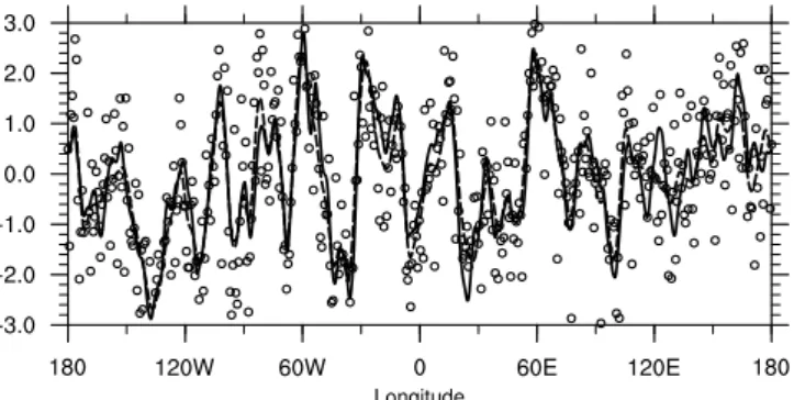
where the length-scale is chosen to be ℓ=250 km; see Michel (2013) for details. The observation operator is a peri-odic linear interpolation. Observations are taken to be equally spaced, which allows easy inclusion of spatial correlations if needed, using the same model as B but in observation space. In order to roughly simulate the characteristics of op-erational data assimilation, the number of variables is taken asn=1000 and there arep=500 observations with preci-sionσo=1 K. The fields are illustrated in Fig. 1. In this par-ticular case, the value of the cost-function at the minimum isJe=245.8≈p/2 as the specified error statistics are fully consistent with the ones of the innovation vector.
3.3 Validation of the randomized trace estimation
The distribution of the observation and background terms at the minimum have been obtained from running 104 indepen-dent realizations of the assimilation scheme. The distribution of the obtained values is shown in Fig. 2. The total cost func-tion has a mean of ≃250.11 which is consistent with the theoretical expectationp/2=250 (within the bounds of a standard confidence interval with 104realizations). The es-timated variances of the observation and background terms are lower than their mean, which is consistent with the dis-cussion in Sect. 2.
The trace estimation algorithm relies on randomization, thus its results depend on the sample size. The algorithm has been applied to compute Tr(HK), Tr(HK)2, and also independently Tr(KH) and Tr(KH)2 for various ensem-ble (sampling) sizesM between 1 and 100. The procedure has been applied 200 times in order to evaluate the sta-tistical properties of the randomized trace estimator. Re-sults are presented in Fig. 3. Almost identical reRe-sults are obtained among ensemble sizes. Averaging over the en-semble sizes and the 200 realizations gives the estima-tions Tr(HK)≃80.15, Tr(KH)≃80.19, Tr(HK)2≃56.7, Tr(KH)2≃56.86 which are obviously consistent when-ever Eq. (26) or Eq. (27) is used. The comparison with
Fig. 1.True signalxt(solid black line), observationsyo(circles)
and the analysis xa (dashed black line) simulated with the
pre-scribed statistics for background and observation errors (see text). The backgroundxbis zero.
Fig. 2.Histograms obtained with 104realizations of the assimila-tion scheme shown in Fig. 1 for the values of(a)the background cost function and(b)the observation cost function at the minimum.
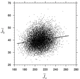
Fig. 3.Scatterplot of the values of the background cost function and the observation cost function at the minimum.
Table 1.Comparison of the simulated optimal innovation method
with the randomized trace estimation, following Eqs. (16), (17), (21), and (22).
E(eJb) 40.01 12Tr(HK) 40.09
Var(Jeb) 28.14 21Tr[(HK)2] 28.41
E(eJo) 210.11 12Tr(I−HK) 209.91
Var(Jeo) 194.38 12Tr[(I−HK)2] 198.24
Differences between theoretical and estimated values arise from sample size. Moving to cross-correlation between the values ofJeoandJeb, the simulated optimal innovation method gives an estimate
Corr Jo,e Jbe≃0.164 (29)
which is also in rather good agreement with the estimation from the trace algorithm:
Tr [HK(I−HK)] q
Tr(HK)2Tr(I−HK)2
≃0.156 (30)
as also shown in Fig. 3;JoeandJbeare positively correlated. Figure 4 shows how the trace estimator becomes more and more precise as the ensemble size goes larger. More pre-cisely, the variance of the estimator (26) is (Chapnik et al., 2006):
Var
1 M
M X
i=1 ηTiAηi
=M1 Tr "A
+AT
2 2#
.
Thus, it is possible to estimate the precision of the ran-domized trace computation as a function of ensemble size
(a)
(b)
Fig. 4. Randomized trace estimation of Tr(HK) (a, squares), Tr[(HK)2](a, circles), Tr[(HK)THK](a, plus signs) and Tr(KH) (b, squares), Tr[(KH)2](b, circles), Tr[(KH)TKH](b, plus signs), as a function of the ensemble size used for the randomization. Solid line: expectation; dashed lines: expectation plus or minus one stan-dard deviation, as determined from a Monte-Carlo approach with 200 independent realizations.
M and as a function of traces Tr(HK)2, Tr(HK)THK, Tr(KH)2 and Tr(KH)TKH which themselves can be computed with the randomized approach proposed in Sect. 3.1. This also implies that while Eqs. (25) and (26) can be applied to estimate Tr(HK)=Tr(KH), both estimators have different precisions, as apparent in Fig. 4.
3.4 Variance tuning
DI01 proposed to adjust multiplicative scaling factorssband sofor the covariance matricesBandR, assuming that at least approximately
Bt=sbB (31)
Rt=soR (32)
the realization of the cost function at the minimum to their expectations:
sb= 2Jeb
Tr(HK) (33)
so= 2Joe
Tr(I−HK) (34)
These equations can be seen as a fixed point relation that is solved iteratively.
Alternatively, if the conditions (31)–(32) are satisfied, then it is also possible to derive an alternative formulation for those coefficients. Indeed, the innovation vector d has covariance
6=HBtHT+Rt=sbHBHT+soR
=
sb−so
HBHT+soD (35)
=sbD+
so−sb
R. (36)
Using Eq. (35) in Eq. (12) withµ=0 gives: 2E Jeb
=TrKTB−1K6
=sbTr
KTB−1KD
+
so−sb
Tr
h
KTHTD−1R i
=sbTr(HK)+
so−sb
Tr [HK(I−HK)] (37) Using Eq. (36) in Eq. (13) withµ=0 gives
2E Jeo
=soTr(I−HK)+sb−soTr [HK(I−HK)] (38) which was already been obtained by Chapnik et al. (2006) when discussing the first iteration of the algorithm designed by DI01. In view of Eqs. (21)–(22), the random fluctuations of Jeb andJeo are small and the expectation can usually be replaced by a single realization. This turns Eqs. (37)–(38) into a linear systemof two unknowns so, sb which can be written as:
αsb+(α−β)
so−sb
=2Jbe (p−α) so+(α−β)
sb−so
=2Joe
and where the notationsα=Tr(HK),β=Tr(HK)2have been introduced for simplification. If the system is not singu-lar, then the unique solution is:
sb=2(β−α)Jeo+(p−2α+β)Jeb
β (p−2α+β)−(β−α)2 (39) so=2 βJeo+(β−α)Jeb
β (p−2α+β)−(β−α)2 (40)
At the price of computing Tr(HK)2, the final solution of DI01’s algorithm can be directly obtained, without any further iteration in the case where specified and true er-ror covariances differ by a scaling factor as indicated by Eqs. (31)–(32). This may however not be the case when ob-servation operators are non-linear or when this condition is not met.
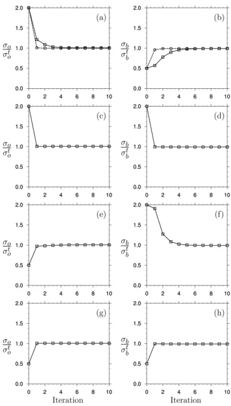
In our setting, Tr(HK)2 is lower but comparable to Tr(HK) in magnitude (see Sect. 3.3 for details). Both traces are smaller by about one order of magnitude with respect to the number of observations, which is consis-tent with recent estimates in ARPEGE (Desroziers et al., 2009, Fig. 1). DI01’s formulation neglects the term (so− sb)Tr [HK(I−HK)] (but the correct estimate is recovered through the iterations). This term is indeed likely to be negli-gible in Eq. (38) but not so in Eq. (37). Thus, more iterations of the scheme may be needed to recover the appropriate value of sb, rather thanso, as already noticed by DI01 (Tables 3 and 4). In contrast, the correct estimate can be obtained by solving the linear system with the direct solution given by Eqs. (39)–(40). The iterative tuning of the coefficients fol-lowing DI01’s approach is shown in Fig. 5 for overestimated or underestimated σo and σb. They confirm that generally, a single iteration is necessary for tuningσo (panels a, c, e, and g). In contrast, around four iterations can be necessary for recovering a useful value ofσbespecially whenso−sbis large (panels b and f), as the term(so−sb)Tr [HK(I−HK)] cannot be neglected. The formulation (39)–(40) recovers the correct factor within one iteration (shown only in panels a and b).
This suggests that it may be useful to use the formulation (39)–(40) when trying to diagnose a multiplicative factor for the background term. This happens for instance for the infla-tion of variances in an ensemble of data assimilainfla-tions (Ray-naud et al., 2012). Extension of this formulation to the simul-taneous tuning of several parameters (corresponding to sub-parts of the background and the observation cost-functions) is possible but more complicated, as a linear system of order S+P (the number of sub-terms) has to be solved. This will be the topic of further studies.
4 Application in the ARPEGE 4D-Var
Fig. 5.Iterative tuning of multiplicative coefficients for the error covariance matrices.σo(left) andσb(right) are tuned simultaneously with(a,
b)overestimatedσo, underestimatedσb;(c, d)overestimatedσoandσb;(e, f)underestimatedσoand overestimatedσb;(g, h)underestimated σoandσb=. Solid lines and square marks: iterative tuning following DI01’s approach; dashed lines and circle marks: new approach (shown
only ina, b). Traces are estimated with the randomization method using 100 independent realizations.
4.1 Estimation of tuning factors
Randomized estimates of the traces are performed in the same way as in the idealized 1-D model using the assimi-lation with perturbed observations. For the background term,
Fig. 6.Diagnosedσo’s-tuning factors per observation type
(September 2013).
factors are therefore estimated in the very same way as in Desroziers et al. (2009). Randomized estimates of the traces have been averaged over a one week period and use a sample sizeM=6, giving the following values:
Tr(HK)≃70 000, Trh(HK)2i≃57 000.
An application of the preceding expressions shows that back-ground error standard deviations are overestimated by a fac-tor 0.85. Thus, the specifiedBmatrix in ARPEGE is closer to its diagnosed value than in previous studies (Desroziers et al., 2009), but stillB<Bt. The estimated values for the observa-tion error standard deviaobserva-tions are shown in Fig. 6 for dif-ferent observation types. Albeit previous studies have high-lighted that observation errors are generally overestimated in data assimilation schemes (possibly because of approximate bias correction or neglect of spatial correlations in the er-rors), this was not the case anymore for some conventional observations (columns DRIFTBUOYS and RADIOSOUND-ING haveSo=√so>1). As explained by Desroziers et al. (2009), the obtained values for observation types AIR-CRAFT, BRIGHT. TEMP. (satellite measurements) and GP-SRO are suspiciously low and this is probably due to the fact that these observations indeed have correlated errors (thus, additional parameters describing these correlations should be included in the maximum-likelihood approach). In our study the corresponding coefficients will just be discarded for the tuning as in Desroziers et al. (2009).
4.2 Impact in terms of forecast performance
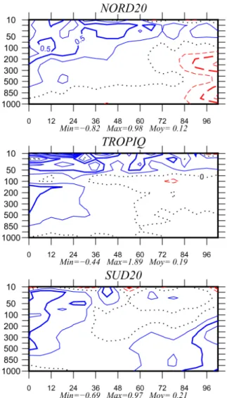
We have investigated the impact of tuning the background and observation variances in the global 4D-Var scheme. Fi-gure 7 shows the differences between root-mean-square er-rors for the geopotential between the reference and the
ex-Fig. 7.Impact of tuning on forecast scores: differences between the root mean squared errors of the reference and of the experiment compared to independent ECMWF analyses (geopotential error in m), as a function of forecast range (in h). NORD20 is the domain on the globe that is north of 20◦N, TROPIQ is the domain between 20◦N and 20◦S, and SUD20 is south of 20◦S. Blue (red) indicates better (worse) performance. The verification period is one month (September 2013).
5 Conclusions
A posteriori diagnostics can help to detect misspecifications in the statistics of a data assimilation scheme. However, it is generally not possible to tell where the misspecification lies unless some further hypotheses are made (Talagrand, 2010).
Among those diagnostics, one is particularly simple. The value of the cost-function at the minimum should be close to its expected valuep/2 wherepis the number of observations (Bennett et al., 1993). It is possible to refine this diagnostic to sub-parts of the cost function (Talagrand, 1999). Despite care taken in the estimation of error covariance matrices, imple-mentation of this diagnostic in early operational data assim-ilation schemes showed that the amplitude of the innovation vector was a priori overestimated by a factor 2–3 as reported by Talagrand (1999), possibly because of the misspecifica-tion of error correlamisspecifica-tions for satellite observamisspecifica-tions.
This paper introduces some additional results using the fact that the sub-parts of the cost function at the minimum can be expressed as quadratic forms of the innovation vector. For some specific distributions of the innovation vector, in-cluding the multivariate normal, expressions for the expecta-tion, variances and cross-covariances can be given. In partic-ular, the observation and background terms at the minimum are positively (generally weakly) correlated (when the inno-vation vector follows the expected statistics).
The expressions involve the trace of larges matrices such as Tr[(HK)2]. It is shown that these matrices can be esti-mated from a randomized method (when K is not explic-itly available) by applying the assimilation scheme twice. The randomized method is shown to yield results that are consistent with the “simulated optimal innovation” method (Chapnik et al., 2006). Finally, it is advocated that the com-putation of Tr[(HK)2]could be useful for variance tuning, in particular for the inflation factor of the background error covariance matrix. Further work will attempt to estimate ad-ditional covariance parameters following Purser and Parrish (2003) and also make use of recent advances in randomized linear algebra (Aune et al., 2012; Stein et al., 2013)
Acknowledgements. Part of this work was stimulated by a pre-sentation given by M. Jardak at the International Conference on Ensemble Methods in Geophysical Sciences, Toulouse, November 2012. I am grateful to F. Rabier and to G. Desroziers for providing helpful comments on a previous version of this manuscript. This study benefited from the support of the RTRA STAE foundation within the framework of the FILAOS project.
Edited by: T. Gneiting
Reviewed by: R. Bannister and E. Aune
The publication of this article is financed by CNRS-INSU.
References
Aune, E., Simpson, D., and Eidsvik, J.: Parameter estimation in high dimensional Gaussian distributions, Stat. Comput., online first, 1–17, doi:10.1007/s11222-012-9368-y, 2012.
Avron, H. and Toledo, S.: Randomized algorithms for estimating the trace of an implicit symmetric positive semi-definite matrix, Journal of the ACM, 58, 8:1–8:34, 2011.
Bannister, R. N.: A review of forecast error covariance statistics in atmospheric variational data assimilation. II: Modelling the forecast error covariance statistics, Q. J. Roy. Meteor. Soc., 134, 1971–1996, 2008.
Bekas, C., Kokiopoulou, E., and Saad, Y.: An estimator for the di-agonal of a matrix, Appl. Numer. Math., 57, 1214–1229, 2007. Belo-Pereira, M. and Berre, L.: The Use of an Ensemble Approach
to Study the Background Error Covariances in a Global NWP Model, Mon. Weather Rev., 134, 2466–2489, 2006.
Bennett, A., Leslie, L., Hagelberg, C., and Powers, P.: Tropical Cy-clone Prediction Using a Barotropic Model Initialized by a Gen-eralized Inverse Method, Mon. Weather Rev., 121, 1714–1729, 1993.
Bennett, A. F., Chua, B. S., Harrison, D. E., and McPhaden, M. J.: Generalized Inversion of Tropical Atmosphere-Ocean (TAO) Data and a Coupled Model of the Tropical Pacific. Part II: The 1995 La Nina and 1997 El Nino, J. Climate, 13, 2770–2785, 2000.
Chapnik, B., Desroziers, G., Rabier, F., and Talagrand, O.: Prop-erties and first application of an error-statistics tuning method in variational assimilation, Q. J. Roy. Meteor. Soc., 130, 2253– 2275, 2004.
Chapnik, B., Desroziers, G., Rabier, F., and Talagrand, O.: Diagno-sis and tuning of observational error in a quasi-operational data assimilation setting, Q. J. Roy. Meteor. Soc., 132, 543–565, 2006. Courtier, P., Thépaut, J.-N., and Hollingsworth, A.: A strategy for operational implementation of 4D-Var, using an incremental ap-proach, Q. J. Roy. Meteor. Soc., 120, 1367–1387, 1994. Courtier, P., Andersson, E., Heckley, W., Vasiljevic, D., Hamrud,
M., Hollingsworth, A., Rabier, F., Fisher, M., and Pailleux, J.: The ECMWF implementation of three-dimensional variational assimilation (3D-Var). I: Formulation, Q. J. Roy. Meteor. Soc., 124, 1783–1807, 1998.
Daley, R.: Estimating observation error statistics for atmospheric data assimilation, Annales Geophysicae, 11, 634–647, 1993. Dee, D. and da Silva, A.: Maximum-Likelihood Estimation of
Forecast and Observation Error Covariance Parameters. Part I: Methodology, Mon. Weather Rev., 127, 1822–1834, 1999. Dee, D. P.: On-line Estimation of Error Covariance Parameters for
Atmospheric Data Assimilation, Mon. Weather Rev., 123, 1128– 1145, 1995.
Desroziers, G. and Ivanov, S.: Diagnosis and adaptive tuning of observation-error parameters in a variational assimilation, Q. J. Roy. Meteor. Soc., 127, 1433–1452, 2001.
Desroziers, G., Berre, L., Chabot, V., and Chapnik, B.: A posteriori diagnostics in an ensemble of perturbed analyses, Mon. Weather Rev., 137, 3420–3436, 2009.
Evensen, G.: The Ensemble Kalman Filter: theoretical formula-tion and practical implementaformula-tion, Ocean Dynam., 53, 343–367, 2003.
Fisher, M.: Background error covariance modelling, in: ECMWF Seminar on recent developments in data assimilation for atmo-sphere and ocean, ECMWF, 45–63, 2003.
Gauthier, P. and Thépaut, J.-N.: Impact of the digital filter as a weak constraint in the preoperational 4Dvar assimilation system of Météo-France, Mon. Weather Rev., 129, 2089–2102, 2001. Gauthier, P., Charette, C., Fillion, L., Koclas, P., and Laroche, S.:
Implementation of a 3D variational data assimilation system at the Canadian Meteorological Centre. Part I: The global analysis, Atmos. Ocean, 37, 103–156, 1999.
Genton, M. G., He, L., and Liu, X.: Moments of skew-normal ran-dom vectors and their quadratic forms, Stat. Probabil. Lett., 51, 319–325, 2001.
Girard, D.: Asymptotic optimality of the fast randomized versions of GCV and CL in ridge regression and regularization, Ann. Stat., 19, 1950–1963, 1991.
Guidard, V. and Fischer, C.: Introducing the coupling information in a limited-area variational assimilation, Q. J. Roy. Meteor. Soc., 134, 723–735, 2008.
Hollingsworth, A. and Lonnberg, P.: The statistical structure of short-range forecast errors as determined from radiosonde data. Part I: The wind field, Tellus A, 38, 111–136, 1986.
Houtekamer, P. and Mitchell, H.: A Sequential Ensemble Kalman Filter for Atmospheric Data Assimilation, Mon. Weather Rev., 129, 123–137, 2001.
Hutchinson, M. F.: A stochastic estimator of the trace of the in-fluence matrix for Laplacian smoothing splines, Commun. Stat.-Simul. C., 18, 1059–1076, 1989.
Kucukkaraca, E. and Fisher, M.: Use of analysis ensembles in estimating flow-dependent background error variances, Tech. Rep. 492, ECMWF Technical Memorandum, 2006.
Le Dimet, F. X. and Talagrand, O.: Variational algorithms for anal-ysis and assimilation of meteorological observations: theoretical aspects, Tellus A, 38, 97–110, 1986.
Lorenc, A. C.: Analysis methods for numerical weather prediction, Q. J. Roy. Meteor. Soc., 112, 1177–1194, 1986.
Lorenc, A. C.: Development of an operational variational assimila-tion scheme, J. Meteorol. Soc. Jpn, 75, 339–346, 1997. Mathai, A. and Provost, S. B.: Quadratic forms in random variables:
theory and applications, Marcel Dekker, Inc. New York, statis-tics, a series of textbooks and monographs, 1992.
Mathai, A., Provost, S., and Hayakawa, T.: Bilinear Forms and Zonal Polynomials, Springer-Verlag, New York, Lect. Notes Stat., 102, doi:10.1007/978-1-4612-4242-0, 1995.
Ménard, R. and Chang, L.-P.: Assimilation of Stratospheric Che-mical Tracer Observations Using a Kalman Filter. Part II:χ2 -Validated Results and Analysis of Variance and Correlation Dy-namics, Mon. Weather Rev., 128, 2672–2686, 2000.
Ménard, R., Cohn, S. E., Chang, L.-P., and Lyster, P. M.: Assim-ilation of Stratospheric Chemical Tracer Observations Using a Kalman Filter. Part I: Formulation, Mon. Weather Rev., 128, 2654–2671, 2000.
Michel, Y.: Estimating deformations of random processes for corre-lation modelling: methodology and the one-dimensional case, Q. J. Roy. Meteor. Soc., 139, 771–783, 2013.
Muccino, J. C., Hubele, N. F., and Bennett, A. F.: Significance test-ing for variational assimilation, Q. J. Roy. Meteor. Soc., 130, 1815–1838, 2004.
Pailleux, J., Geleyn, J.-F., and Legrand, E.: La prévision numérique du temps avec les modèles Arpege et Aladin: Bilan et perspec-tives = Numerical weather prediction with the models Arpege and Aladin; assessment and prospects, La Météorologie, 32–60, 2000 in French.
Parrish, D. and Derber, J.: The National Meteorological Cen-ter’s Spectral Statistical-Interpolation Analysis System, Mon. Weather Rev., 120, 1747–1763, 1992.
Purser, R. J. and Parrish, D. F.: A Bayesian technique for estimat-ing continuously varyestimat-ing statistical parameters of a variational assimilation, Meteorol. Atmos. Phys., 82, 209–226, 2003. Rabier, F.: Overview of global data assimilation developments in
numerical weather-prediction centres, Q. J. Roy. Meteor. Soc., 131, 3215–3233, 2005.
Rabier, F., Jarvinen, H., Klinker, E., Mahfouf, J.-F., and Sim-mons, A.: The ECMWF operational implementation of four-dimensional variational assimilation. I: Experimental results with simplified physics, Q. J. Roy. Meteor. Soc., 126, 1143–1170, 2000.
Rasmussen, C. E. and Williams, C.: Gaussian Processes for Ma-chine Learning, the MIT Press, 2006.
Raynaud, L., Berre, L., and Desroziers, G.: Accounting for model error in the Météo-France ensemble data assimilation system, Q. J. Roy. Meteor. Soc., 138, 249–262, 2012.
Saad, Y.: Iterative Methods for Sparse Linear Systems, 2nd Edn., Society for Industrial and Applied Mathematics, Philadelphia, PA, USA, 2003.
Sadiki, W. and Fischer, C.: A posteriori validation applied to the 3D-VAR Arpege and Aladin data assimilation systems, Tellus A, 57, 21–34, 2005.
Simmons, A. and Hollingsworth, A.: Some aspects of the improve-ment in skill of Numerical Weather Prediction, Q. J. Roy. Meteor. Soc., 128, 647–677, 2002.
Stein, M. L., Chen, J., and Anitescu, M.: Stochastic Approximation of Score Functions for Gaussian Processes, Ann. Appl. Stat., 7, 1162–1191, 2013.
Talagrand, O.: A posteriori verification of analysis and assimilation algorithms, in: Workshop on diagnosis of data assimilation sys-tems, 2–4 November 1998, ECMWF, Reading, UK, 1999. Talagrand, O.: Data Assimilation: Making Sense of