www.geosci-model-dev.net/6/1989/2013/ doi:10.5194/gmd-6-1989-2013
© Author(s) 2013. CC Attribution 3.0 License.
Geoscientiic
Model Development
An online trajectory module (version 1.0) for the nonhydrostatic
numerical weather prediction model COSMO
A. K. Miltenberger, S. Pfahl, and H. Wernli
Institute for Atmospheric and Climate Science, ETH Zurich, Switzerland Correspondence to:A. K. Miltenberger ([email protected])
Received: 29 January 2013 – Published in Geosci. Model Dev. Discuss.: 21 February 2013 Revised: 4 October 2013 – Accepted: 9 October 2013 – Published: 13 November 2013
Abstract.A module to calculate online trajectories has been implemented into the nonhydrostatic limited-area weather prediction and climate model COSMO. Whereas offline tra-jectories are calculated with wind fields from model out-put, which is typically available every one to six hours, on-line trajectories use the simulated resolved wind field at ev-ery model time step (typically less than a minute) to solve the trajectory equation. As a consequence, online trajectories much better capture the short-term temporal fluctuations of the wind field, which is particularly important for mesoscale flows near topography and convective clouds, and they do not suffer from temporal interpolation errors between model output times. The numerical implementation of online tra-jectories in the COSMO-model is based upon an established offline trajectory tool and takes full account of the horizontal domain decomposition that is used for parallelization of the COSMO-model. Although a perfect workload balance can-not be achieved for the trajectory module (due to the fact that trajectory positions are not necessarily equally distributed over the model domain), the additional computational costs are found to be fairly small for the high-resolution simula-tions described in this paper. The computational costs may, however, vary strongly depending on the number of trajec-tories and trace variables. Various options have been imple-mented to initialize online trajectories at different locations and times during the model simulation. As a first applica-tion of the new COSMO-model module, an Alpine north foehn event in summer 1987 has been simulated with hori-zontal resolutions of 2.2, 7 and 14 km. It is shown that low-tropospheric trajectories calculated offline with one- to six-hourly wind fields can significantly deviate from trajecto-ries calculated online. Deviations increase with decreasing model grid spacing and are particularly large in regions of
deep convection and strong orographic flow distortion. On average, for this particular case study, horizontal and vertical positions between online and offline trajectories differed by 50–190 km and 150–750 m, respectively, after 24 h. This first application illustrates the potential for Lagrangian studies of mesoscale flows in high-resolution convection-resolving simulations using online trajectories.
1 Introduction
1980s, when good-quality and well-resolved gridded wind fields became available. They are nowadays considered to be the most accurate type of trajectories in the troposphere (Stohl and Seibert, 1998).
From the early studies on, the Lagrangian perspective had a large impact on the advance of the understanding of atmo-spheric processes, as it for instance allowed the identification of coherent air streams within extratropical cyclones, most prominently the warm conveyor belt (e.g., Whitaker et al., 1988; Wernli and Davies, 1997). Lagrangian studies were also important to connect ozone-rich episodes in the tropo-sphere to stratospheric intrusions (e.g., Buzzi et al., 1984) or to illustrate the flow blocking at mountain ranges during the passage of fronts (e.g., Buzzi and Tibaldi, 1978; Steinacker, 1984; Kljun et al., 2001). Since trajectory calculations are computationally cheap, the Lagrangian approach is also very valuable to assess the climatological frequency and geo-graphical distribution of atmospheric flow features like warm conveyor belts (e.g., Eckhardt et al., 2004) or stratosphere– troposphere exchange (e.g., Sprenger and Wernli, 2003). But trajectory analysis has also made its way into other fields of atmospheric sciences: for instance, it has been successfully used for analyzing the detailed microphysical evolution of clouds along the flow (e.g., Haag and Kärcher, 2004; Hoyle et al., 2005; Brabec et al., 2012), identifying evaporative wa-ter sources for precipitation (e.g., Bertò et al., 2004; Sode-mann et al., 2008), interpreting measurements of stable wa-ter isotopes (Pfahl and Wernli, 2008) and in studies on atmo-spheric chemistry (e.g., Coude-Gaussen et al., 1987; Miller, 1987; Forrer et al., 2000; Methven et al., 2006). Lagrangian particle dispersion models have been successfully used for modeling the dispersion of atmospheric tracers and pollu-tants (e.g., Gross et al., 1987; Bellasio et al., 2012; Weil et al., 2012).
Besides these large-scale applications of trajectory analy-sis, Lagrangian parcel models have also been applied to study single events in high-resolution numerical models, e.g., for studying hurricane eye dynamics (Stern and Zhang, 2013), the origin of air parcels feeding convective cells (Wang and Xue, 2012) or nocturnal equatorial oceanic squall lines (Fierro et al., 2009). The Lagrangian approach has also been successfully used for analyzing stratocumulus clouds and en-trainment rates in large eddy simulations (LES) (e.g., Stevens et al., 1996; Kogan, 2006; Yamaguchi and Randall, 2012; Yeo and Romps, 2013).
While frequently employed in all fields of meteorology, the accuracy of trajectories derived from measured or mod-eled wind data is a long-standing point of discussion (e.g., Danielsen, 1961; Kahl, 1993; Stohl, 1998; Brioude et al., 2012). The comparison of computed trajectories to the actual path of an air parcel in the atmosphere is difficult, but several attempts have been made, for instance, with the aid of tracer experiments (e.g., Draxler, 1987; Haagenson et al., 1990; van Dop et al., 1998) and balloon or tetroon flights (e.g., Djuric, 1961; Reisinger and Mueller, 1983; Stohl and Koffi, 1998).
In addition to these experiments different trajectory models have been compared (e.g., Stohl et al., 2001), the sensitivity to the input data frequency has been tested (e.g., Rolph and Draxler, 1990; Doty and Perkey, 1993; Stohl et al., 1995) and the errors associated with the numerical scheme have been investigated (Seibert, 1993). In the case of three-dimensional kinematic trajectories, which are usually based on wind data from a reanalysis data set or a weather forecast, several error sources can be identified (Stohl, 1998):
1. truncation errors – due to neglecting higher order terms in the Taylor expansion of the trajectory equation; 2. interpolation errors – due to the interpolation of the
wind field data from the model grid and model output times to the actual trajectory position in space and time 3. wind field errors – due to the nonrepresentativity of the model wind field, prediction errors and errors in the initial conditions.
The third error source depends largely on the quality of the entire forecasting system and the precision of the initial con-ditions, which are independent of the trajectory model. The truncation error depends on the numerical scheme used for solving the trajectory equation. All of today’s frequently used trajectory models – FLEXPART (Stohl et al., 2005), HYS-PLIT (Draxler and Hess, 1998), TRAJKS (Scheele et al., 1996), and LAGRANTO (Wernli and Davies, 1997) – em-ploy the Petterssen scheme (Petterssen, 1940), which is a second-order second-order scheme with a truncation error proportional to 1t2. For further discussion of the numeri-cal properties the reader is referred to Seibert (1993). Seib-ert (1993) argued that the truncation error should clearly be smaller than the overall trajectory uncertainty, and that the time step should be small enough to fulfill the Courant– Friedrich–Levy criterion, which is a prerequisite for conver-gent solutions. With a strongly decreasing grid spacing in recent numerical weather prediction models this constrains the time step to some minutes to seconds. All of the above-mentioned models compute the trajectories based on winds from weather forecasts or reanalysis data sets. Typically, out-put from global models (analyses and forecasts) is avail-able every six hours, and from regional models every hour. As integration time steps of this order would induce unac-ceptably large errors, temporal interpolation between these output times is required for calculating trajectories. The er-rors introduced by temporal and spatial interpolation depend strongly on the spatial and temporal resolution of the wind data. While the spatial resolution of numerical weather pre-diction models has strongly increased over the past years, the output frequency has increased only slowly and therefore often constitutes the limiting factor for a reduction of the in-terpolation error.
solved “online”, i.e., during the integration of the Eulerian numerical weather prediction model. In this case the wind fields are available at every time step of the Eulerian model, which is some tens of seconds in state-of-the-art regional weather prediction models. Consequently, with this approach a large increase in data resolution is obtained compared to the standard approach of calculating “offline” trajectories. How-ever, while offline trajectories can be computed forward or backward in time, with the online approach the trajectory equation can only be solved forward in time.
The first implementation of online trajectories we know of has been accomplished by Rössler et al. (1992). More re-cently the online computation of air parcel trajectories has been utilized in chemistry models within a Lagrangian ad-vection scheme for trace gases (e.g., Becker and Keuler, 2001; Reithmeier and Sausen, 2002). In some studies air par-cel trajectories are constructed based on passive tracer fields, which also makes use of the resolved and subgrid-scale wind fields at each time step of the Eulerian model (e.g. Gheusi and Stein, 2002; Duffourg and Ducrocq, 2011). Rössler et al. (1992) showed in a case study that the increased data in-put frequency indeed significantly alters the pathways of air parcels, particularly over strongly structured topography. In addition to the expected improvement of the trajectory posi-tion found by Rössler et al. (1992), the online computaposi-tion of trajectories may better capture the small-scale variability of the vertical wind field as it is represented on the grid of the Eulerian numerical model. As shown in recent studies by Grell et al. (2004) and Brioude et al. (2012), this is espe-cially relevant for regional weather prediction models with a high spatial resolution. A good representation of the small-scale structure of the wind field is important for investiga-tions of orographic flow and deep convection and for studies using the Lagrangian approach to investigate the evolution of clouds or chemical substances it is essential to capture the vertical wind fluctuations: for instance, the number of homo-geneously nucleating ice crystals is very sensitive to the cool-ing rates along the trajectory (e.g., Kärcher and Lohmann, 2002; Hoyle et al., 2005; Spichtinger and Krämer, 2013).
In this paper we describe a new implementation of the on-line computation of trajectories based on grid-scale wind ve-locities in the regional weather prediction model COSMO (Sect. 2). To illustrate the capabilities of the online trajectory approach, the module is used in a simulation of an Alpine foehn event in July 1987, which is described in Sect. 3. We provide a comparison of the online trajectories to offline tra-jectories based on COSMO-model output at different output frequencies between one and six hours, with a particular em-phasis on the representation of the foehn flow. In addition we investigate the dependence of the detected differences be-tween online and offline trajectories on the horizontal grid spacing of the COSMO-model (14, 7 and 2.2 km). Finally, in Sect. 4, potentials of and challenges for the online computa-tion of trajectories are discussed.
2 The online trajectory module
The goal of our work has been to construct a new mod-ule for the numerical weather prediction model COSMO, which allows calculating forward online trajectories and trac-ing user-specified variables along these trajectories. For the implementation of the online trajectory module, two existing model codes are combined: on the one hand we select the numerical weather prediction model COSMO as the Eule-rian model into which the online trajectory calculation should be embedded. The COSMO-model is a limited-area, nonhy-drostatic model (Baldauf et al., 2011) that is used for high-resolution operational weather forecasting by several mainly European weather services (e.g., the German Meteorolog-ical Service (DWD) and MeteoSwiss). On the other hand we base the trajectory calculation procedure (time stepping as well as interpolation) on the trajectory tool LAGRANTO (Wernli and Davies, 1997), which has been employed in nu-merous studies to compute offline trajectories (e.g., Wernli and Davies, 1997; Stohl et al., 2001; Lefohn et al., 2011; Cirisan et al., 2013; Grams et al., 2013). The LAGRANTO source code has been modified to be consistent with the COSMO-model, the temporal interpolation has been omitted and it has been parallelized to account for the spatial domain decomposition of the COSMO-model.
initialize model
DO t = nstart, nend
forward timestep of Eulerian model
DO i = 1, ntra
IF traj in my domain
Calculate new position
Store data in sendbuffer and determine receiver
T F
IF traj in my domain
F T
Communication between processors
IF output timestep
Write output T
F
finalize model run
Calculate trace variables
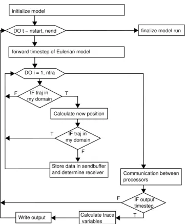
Fig. 1.Flowchart of the online trajectory module for the COSMO-model.
The general workflow inside the module and its embed-ding in the existing model is illustrated by the flow chart in Fig. 1: after initialization of the COSMO-model and the tra-jectory module (Sect. 2.3), the model loops through the time steps of the integration. At the end of each time step the tra-jectory module is called to calculate the new tratra-jectory posi-tions (Sect. 2.1). Then the necessary interprocessor commu-nication takes place (Sect. 2.2), and finally, if the time step is an output time step, the trace variables are interpolated to the trajectory positions and are together with the trajectory posi-tion written to the output files. The module is written in For-tran 90. For the inter-processor communication the MPICH implementation (www.mpich.org) of the MPI library is used. 2.1 Trajectory integration scheme
The physical core has to solve the trajectory equation Dx
Dt =
u(x, t ). For the solution of this equation we employ the
Pet-terssen scheme (PetPet-terssen, 1940), which computes the new trajectory position at timet1=t0+1t from the externally
specified velocityu(x, t )using a second-order semi-implicit
discretization in space and time:
x(ti+1)=x(ti)+1t˙
x(x(ti), ti)+x˙(x(ti+1), ti+1)
2 =x(ti)+1t
u(x(ti), ti)+u(x(ti+1), ti+1)
2 . (1)
This implicit equation for the new positionx(ti+1)can be
rewritten in fix-point iteration form:
xn(ti+1)=x(ti)+1t
u(x(ti), ti)+u(xn−1(ti+1), ti+1)
2 . (2)
For the required starting values, x0(ti+1) and u(x0(ti+1), ti+1), x(ti) and u(x(ti), ti) are used in the
Petterssen scheme. Therefore, the Petterssen scheme can also be viewed as a predictor–corrector method that ap-proximates the velocity for the forward integration by the mean wind between two successive trajectory locations. Expanding the iteration and dropping the explicit time dependency ofxyields
x1(ti+1)≈x(ti)+1tu(x, ti), (3)
x2(ti+1)≈x(ti)+1
21t (u(x, ti)+u(x1, ti+1)) , (4)
. . . (5)
xn(ti+1)≈x(ti)+1
21t (u(x, ti)+u(xn−1, ti+1)) . (6) The new trajectory position is calculated with this scheme at every main model time step of the COSMO-model, which is usually 20 s for simulations with a grid spacing of 2.2 km and 40 s with a grid spacing of 7 km. We choose the Pet-terssen scheme because it is used by all of the frequently used trajectory models, because it is accurate to the second order and because several studies have shown that higher or-der schemes do not perform essentially better (e.g., Seibert, 1993). It should be noted that the Petterssen scheme is a so-called “constant acceleration” solution; that is, it neglects the change in acceleration of the air parcel during an integration time step. However, we think that this assumption is justi-fied in the online computation even more than in the offline calculation because of the very small integration time step.
The convergence of the Petterssen scheme depends on the properties of the flow field and the starting values for the it-eration. Seibert (1993) showed that fulfilling the Courant– Friedrich–Levy (CFL) criterion is important for obtaining a convergent solution of the trajectory equation. Assuming a maximum wind velocity of 50 m s−1, the horizontal CFL
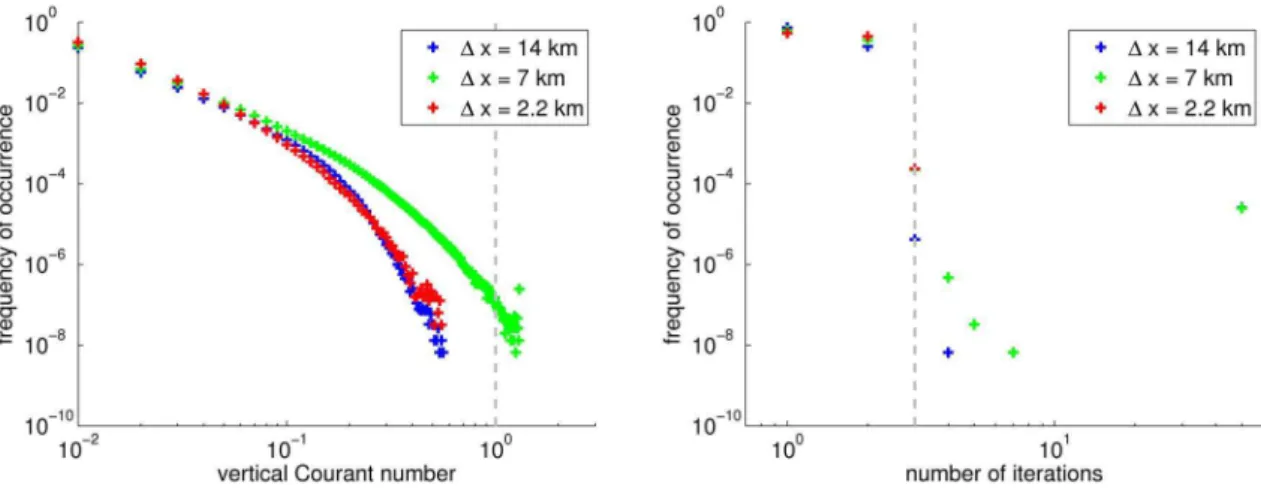
cri-terion requires the time step to be smaller than 280 s for a grid spacing of 14 km and below 40 s for a grid spacing of 2 km. The main model time step, at which the trajectory inte-gration is performed, is smaller than these values in the stan-dard COSMO-model setup. In the vertical the CFL criterion is also almost always fulfilled in our test simulations (Fig. 2, left panel).
Fig. 2.Left: distribution of the vertical Courant numbers during all integration and iteration steps during the simulation of our Alpine case study. Right: number of iterations required until the solution of the trajectory equation converges. The criterion for convergence is that the horizontal position change by less than one-tenth of the horizontal grid spacing and less then 1 m in the vertical.
results are summarized in Fig. 2 (right panel) for simulations with three different horizontal resolutions: in almost all cases the solution converges in the first few iteration steps. Only in about 0.1 ‰ of all time steps more than seven iterations are required, but in these instances the solution is probably truly nonconvergent as the iteration does not stop during the first 50 cycles. Based on these results we choose a default value of three iterations. However, it is possible to adapt this number via the namelist.
The trajectory position is written to the output at a user-specified multiple of the major COSMO-model time step to-gether with the variables traced along the trajectories. The values of the trace variables are obtained by interpolation, as described in the next section, from the Eulerian grid to the trajectory position. The trace variables can be defined by the user via the name list.
2.2 Interpolation, lower boundary condition and terrain intersection problem
The Petterssen scheme requires the velocity u(x, t ) at the
parcel location at each integration time step, and therefore an interpolation of the wind data from the Eulerian grid to the parcel position is necessary. We decided to use a three-dimensional linear interpolation as it is, for instance, also used in LAGRANTO. The interpolation is performed be-tween the eight neighboring grid points of the trajectory position along the coordinate axes of the COSMO-model; that is, the horizontal interpolation is done along terrain-following surfaces. Higher order interpolation is used by some other trajectory models (e.g., FLEXPART, optional in LAGRANTO), but may not always give better results. More-over the errors introduced by the linear interpolation are much easier to interpret. In contrast to existing offline mod-els, no temporal interpolation of the wind field is required as
it is available at each model time step, which is for online trajectories identical to the trajectory integration time step.
Since the COSMO-model uses a staggered Arakawa C grid, the question arises as to how to derive the wind field as well as other parameters close to the surface, i.e. below the lowest model level but above the surface. This question is also strongly linked to the formulation of the lower bound-ary condition. In the current version we decided to use a lin-ear extrapolation of the horizontal wind velocity components from the two lowest model levels as it is for instance used, as one option, in the fast wave solver of the COSMO-model. The vertical velocity is calculated by terrain-following linear interpolation.
0 2 4 6 8 10 12 0
100 200 300 400 500
x [km]
z [m]
topography online traj. dt = 1s offline traj. dt = 5.3 min
Fig. 3.Illustration of the terrain intersection problem. For the cal-culation a zig-zag-shaped topography is assumed (black line). The wind is assumed to be terrain following and linearly increasing with elevation above ground: the horizontal velocity is 3 m s−1at the first level, which is 10 m above the surface and 6 m s−140 m above the surface. The vertical velocity is calculated such that the wind is ter-rain following on all levels. The horizontal velocity at the surface is obtained by linear vertical extrapolation from the two levels above, and the vertical velocity at the surface is calculated from this extrap-olated velocity. If the air parcel is advected below the topography, the wind components at the surface are used. The blue line shows the calculated online trajectory (time step of 1 s) and the cyan line an offline trajectory (time step of 5.3 min).
following wind field, which increases with height (Fig. 3). The velocity at the lowest model level is assumed to be nonzero but terrain following. As is well visible in Fig. 3, the horizontal interpolation smooths the wind field, and therefore the “online” (blue) as well as the “offline” (cyan) trajectory do not follow the terrain at a constant distance. In the exam-ple of the “offline” trajectory, this does not lead to a detected terrain intersection as the trajectory points up- and downwind of the peak are above topography. The online trajectory has, due to the shorter time step, much more points and therefore the intersection even with this narrow peak is detected.
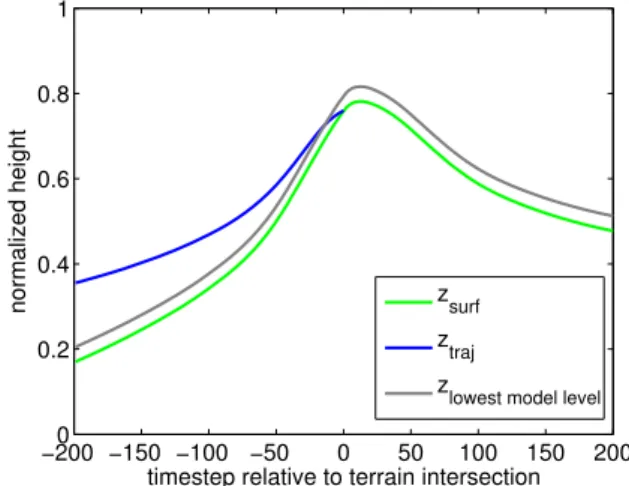
To investigate our third point from above in more detail, we have constructed a composite of the terrain, the trajectory elevation and the height of the lowest model level for all tra-jectories that hit the topography in the case study described in Sect. 3 (Fig. 4). In the last 200 time steps before terrain in-tersection, the surface elevation as well as the lowest model level are traced along these trajectories. In addition the ele-vation of the surface, which would be beneath the trajectory if it continued in the same direction and with the same speed as during the last time steps before the terrain intersection, was computed for the next 200 time steps. The composite was constructed by normalizing the data with the maximum elevation along each trajectory segment and averaging. The situation revealed by the composite analysis (Fig. 4) shows a trajectory passing over a narrow peak, as the 400 time steps
−200 −150 −100 −500 0 50 100 150 200 0.2
0.4 0.6 0.8 1
timestep relative to terrain intersection
normalized height zsurf
ztraj
z
lowest model level
Fig. 4.Composite of the surface elevation (green), trajectory height (blue) and lowest model level (grey) for all terrain intersecting tra-jectories in the COSMO7 simulation of our Alpine case study.
correspond to an average travel distance of about 3 to 6 grid points. Hence the composite closely resembles the picture constructed above with the idealized “zig-zag” topography, which indicates that horizontal interpolation is one factor contributing to terrain intersections. The strong reduction of the time step from offline to online calculation of trajecto-ries increases the frequency of detection of such events and therefore explains the higher percentage of terrain hitting tra-jectories.
The composite analysis indicates that the smoothing of the wind field by horizontal interpolation may play a role, but other possible explanations such as the formulation of the lower boundary condition and the choice of the start-ing values used for the fix-point iteration in the Petterssen scheme cannot be ruled out. Another option for the lower boundary condition would be to useu=v=w=0 m s−1at
the moment being we have adopted the approach of other of-fline trajectory tools to artificially place every parcel hitting the topography at a point 10 m above the surface.
2.3 Parallelization and communication
The COSMO-model employs a spatial grid decomposition for the computation on multiprocessor machines, which con-stitutes a major difficulty for introducing the trajectory calcu-lation: in contrast to the Eulerian model, for which the grid points have a fixed spatial position – that is, they remain asso-ciated with a certain processor during the entire integration – trajectories have no fixed spatial position and hence may pass from the spatial domain associated with a certain pro-cessor to another domain. This problem increases the inter-processor communication significantly, which may deterio-rate the model performance on multiprocessor machines. In addition the trajectories may not be equally distributed in space at each time instant, which makes it impossible to ob-tain a workload balance without strongly modifying the ex-isting COSMO-model structure. However, the effects of the workload imbalance may not strongly affect the model per-formance because usually the number of operations needed on a certain processor to compute the new trajectory posi-tions is much smaller than the number of operaposi-tions required at the Eulerian grid points. To ensure a perfect workload bal-ance, it would be necessary to either perform the trajectory integration on processors that are not associated with the do-main in which the trajectory is located or to reassign Eule-rian grid points to different processors at each time step. In both cases parts of the Eulerian variable fields have to be exchanged between processors during each time step. This additional communication is computationally expensive and would offset the effect of a perfect workload balance in al-most all applications. We therefore decided to keep a fixed spatial domain decomposition and a corresponding associa-tion of trajectories.
The trajectory locations are stored in an array that is a pri-ori known to all processors. A certain processor works only on the entries corresponding to trajectories inside its domain. However, in order to minimize the communication, the tra-jectory array is only updated at the processor that performs the integration, and in case a trajectory passes to the domain of another processor, the information is transferred to this other processor. As illustrated in Fig. 1 all communications are performed when all processors have finished the forward integration. Therefore a minimum number of communication operations is obtained, and the communication overhead is kept small. Additional communication is required if output has to be written at a certain time step because then the entire trajectory array on the processor responsible for the IO has to be updated. In some cases with very few trajectories pass-ing between processors, a complete update of the trajectory array on all processors after each time step may be faster due to a smaller relative communicational overhead. Therefore
this option is also implemented. For all communications the MPI library is used as in the entire COSMO-model.
2.4 Selection of trajectory starting points
An essential choice made by the user of the online trajectory module is the specification of the starting points of the trajec-tories. This is not a trivial task as no backward computation is possible and hence an a priori knowledge of the interest-ing startinterest-ing regions and times is required. Startinterest-ing trajecto-ries at all grid points and time steps is not feasible for high-resolution models due to storage limitations and because it will very strongly increase the runtime of the model. In the present version several options to specify the starting region are available:
– start trajectories once at each grid point inside a rect-angular box (via namelist);
– start trajectories once at user-specified coordinates (via external file);
– start trajectories repeatedly at fixed locations at user-specified times (via namelist);
– start trajectories repeatedly at fixed locations at a reg-ular time interval (via namelist); and
– start trajectories at different locations at different times (via external file).
A detailed description is provided in the Supplement.
3 Results from an Alpine case study
For a first application of the new online trajectory module we simulate the meteorological evolution over central Eu-rope from 25 to 29 July 1987, which has already been inves-tigated by Rössler et al. (1992), Buzzi and Alberoni (1992) and Paccagnella et al. (1992).
3.1 Meteorological situation
rotated longitude
rotated latitude
1010
1010
1010
1010
1010
1010
1010 1010
1010
10 1
1010
1010 101
0 1010
1016
1016
1016
1016
1016
101 6
101 6
1022
1022
1022
1028
−10 −5 0 5 10
−10 −5 0 5 10
0 0.5 1 1.5 2 3 6 9
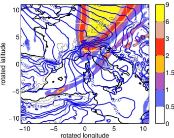
Fig. 5.The potential vorticity distribution on the 320 K isentropic surface is shown in colors (in pvu) and the sea-level pressure field in blue contours (every 2 hPa) at 18:00 UTC, 26 July 1987 based on the COSMO14 simulation.
In addition a moderate Alpine lee cyclone developed over the Adriatic Sea, which was influenced by the retardation and deformation of the cold front by the Alpine ridge (Buzzi and Alberoni, 1992). For the trajectory analysis we focus on the time period during which the cold front passes the Alps, i.e., the afternoon and evening of 26 July 1987.
3.2 Modeling framework
For the numerical simulations of the case study, the COSMO-model version 4.17 (Baldauf et al., 2011) is used with three different spatial resolutions: two with 40 vertical levels and a horizontal grid spacing of 14 km (0.125◦, 195×200 grid points, COSMO14) and 7 km (0.0625◦, 390×400 grid points, COSMO7), respectively, and one with 60 verti-cal levels and a horizontal grid spacing of 2.2 km (0.02◦,
1190×1220 grid points, COSMO2.2). The spacing of the vertical levels ranges from approximately 16 m (13 m) close to the surface to 2800 m (1190 m) at 23 km, i.e. the model top, with an average of 582 m (388 m) for COSMO14 and COSMO7 (COSMO2.2). The domain reaches from approxi-mately 30◦N to 55◦N and from 7◦W to 25◦E, with the pole
of the rotated grid lying at 47.5◦N and−171.5◦E. We
em-ploy the standard model setup of the Swiss weather service except for the microphysical parameterization, for which the two-moment scheme with six hydrometeor classes by Seifert and Beheng (2006) is used. Turbulence, soil processes and radiation are parameterized in all simulations. For the COSMO2.2 simulation only shallow convection is parame-terized, while in the other simulations also deep convection is parameterized with the Tiedtke convection scheme. The time step is 20 s for COSMO2.2 and 40 s for the two other setups. The boundary and initial conditions for COSMO14
and COSMO7 are derived from the ERA-40 reanalysis with a spatial resolution of T159 (Uppala et al., 2005), while COSMO2.2 is driven by the COSMO7 simulation. There-fore the COSMO2.2 simulation is performed over a slightly smaller geographical domain. The COSMO14 and COSMO7 simulations are started at 00:00 UTC on 25 July 1987; COSMO2.2 is started two hours later. All simulations end at 00:00 UTC on 29 July 1987. To assess the computational performance, each simulation is performed twice, once with and once without the online trajectory module.
At 02:00 UTC on 25 July 1987 in total 24 615 trajecto-ries are started over the British Isles at each grid point be-tween 50◦and 54◦N and−5◦and 2◦E and each model level
from the surface up to 5 km. According to the distribution of vertical levels in the Gal-Chen hybrid coordinate system this gives about twice as many trajectories starting below 2 km than above.
A comparison of the sea-level pressure, temperature and precipitation evolution simulated by the COSMO-model with the analysis by Buzzi and Alberoni (1992) and Paccagnella et al. (1992) reveals a reasonable performance for all simulations (not shown). The developing lee cyclone is slightly shallower than in the observations and the con-vection over the eastern Po Valley starts about three hours later. Nevertheless, the essential mesoscale phenomena like the foehn flow, a strong mistral and the strong low-level jet around the eastern edge of the Alpine ridge are well captured in the COSMO simulations.
For the evaluation of the trajectory module we also com-pute offline trajectories with LAGRANTO for each model simulation. The offline trajectories are started at the same points and time as the online trajectories. For the integration of the offline trajectories the wind fields from the COSMO simulations are used at output intervals of one, three and six hours and the integration time step is set to one-twelfth of this time interval. Similar to the online trajectory calculation, air parcels are placed 10 m above the surface if they are advected below ground.
3.3 Computational performance of the online trajectory module
To assess the computational performance of the COSMO-model with the online trajectory module, we use the COSMO-model simulations performed for the Alpine case study described in the previous section. The number of processors varies with the spatial resolution of the simulation to obtain reasonable runtimes: 16 for the 14 and 7 km simulations and 128 for the 2.2 km simulation. In addition to the position, 10 additional variables are traced along the online trajectories, and all vari-ables are written to the output files every model time step. Twenty-two three-dimensional and 14 two-dimensional Eu-lerian variables are written to output files every model hour.
Table 1.Relative runtime increase with respect to the named reference simulation for COSMO-model simulations with the online trajectory module for 24615 trajectories and 10 trace variables. The simulations were run using 16 processors (COSMO14 and COSMO7) or 128 processors (COSMO2.2).
1x=14 km 1x=7 km 1x=2.2 km
without trajectory module (reference: COSMO14 without trajectory module) 0.00 3.16 13.2
with trajectory module (reference: COSMO14 without trajectory module) 0.264 3.45 13.6
with trajectory module (reference: simulation without trajectory module) 0.264 0.0681 0.0366
the trajectory module is below 30 % for the 14 km simula-tion, and the impact of the trajectory calculation on the run-time decreases to a few percent for the higher-resolution sim-ulations. This is because the number of trajectories remains constant, while the number of grid points is much larger. The observed runtime increase is not due to the integration of the trajectory equation itself, which is computationally cheap to solve, but is mainly caused by additional writing of out-put, the additional communication between processors and probably in some cases also by the extensive interpolation of trace variables. Of course the expected runtime increase strongly depends on the number of trajectories, the number of traced variables and the number of processors. In general the observed runtime increase is satisfactorily small in this test case.
3.4 Comparison of online and offline trajectories
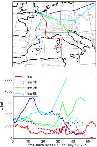
The most prominent mesoscale flow features identified by Buzzi and Alberoni (1992) – the flow splitting at the Alps with a strong low-level wind on either side of the mountain range and the north foehn flow with a particularly strong out-flow from the Simplon–Gotthard region – are well captured by the online and offline trajectory calculations (Fig. 6; foehn trajectories are those passing close to the black cross in both panels). Another interesting feature revealed by the trajectory analysis is the strongly ascending branch of air over eastern Europe, which is associated with ascent ahead of the upper-level trough. Its passage over central Europe is accompanied by trajectories suddenly changing direction from southeast to northeast and rising as, for instance, also observed over the eastern Alps (trajectories rising above 5 km in Fig. 6). A first qualitative impression of the differences between online and offline trajectories can be obtained from Fig. 6: while the flow patterns of the online (bottom panel) and the offline tra-jectories based on three-hourly output (top panel) agree quite well on first order, significant differences are observable if subsynoptic-scale flow patterns are considered. For instance the flow around Corsica shows a much more detailed flow structure in the online trajectories, the ratio of trajectories passing over and around the Massif Central, the Pyrenees and the Alps varies quite strongly, and over the Po Valley, the westward curvature of the online trajectories that crossed the Alps is much stronger than that of the equivalent offline trajectories.
Fig. 6.Offline trajectories based on three-hourly output (top) and online trajectories (bottom) calculated for a COSMO2.2 simulation. Only trajectories starting south of 8.5◦N (rotated coordinates) and between 1400 and 1500 m altitude are shown. The colors denote the height of the trajectories above sea level (in meters). The trajectories that pass close to the black cross are the foehn trajectories in both panels.
(e.g., Rolph and Draxler, 1990; Stohl, 1998). The AHTD de-scribes the average overN trajectories of the horizontal dis-tance between each trajectory calculated with two data sets as a function of time:
AHTD(t )= 1 N
N X
n=1
{Xn(t )−xn(t )}2+ {Yn(t )−yn(t )}20.5, (7) where (xn,yn) is the position of thenth reference trajectory
and (Xn,Yn) the position of thenth test trajectory. The AVTD
is calculated with a similar equation for the trajectory heights
znandZninstead of the horizontal position. Note that AHTD
and AVTD only indicate the mean deviation of all pairs at a certain time. The sensitivity of trajectories with the same starting point to the temporal resolution of the wind field data can vary substantially with the flow features they encounter during their path: as illustrated in Fig. 7, online and offline trajectories sometimes take almost the same path, while at other occasions they diverge strongly and spread over entire Europe. It seems that the closer to the starting point a sen-sitive flow situation is encountered, the larger the final devi-ation. For instance the strongly diverging trajectory bundle shown in Fig. 7 (solid lines) enters a convective region off the coast of northern France. In this case the representation of small-scale vertical velocity structures strongly influences the final three-dimensional path of the parcel. The other set of trajectories shown in Fig. 7 (dashed-dotted lines) does not encounter such a sensitive situation and remains fairly coher-ent.
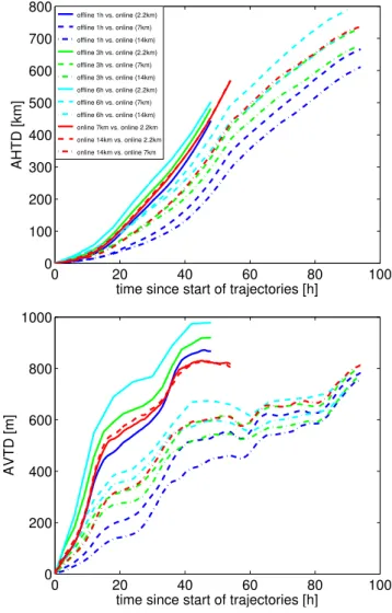
AHTD and AVTD were computed with the online trajec-tories as the reference data set and offline trajectrajec-tories as the test data set for all spatial and temporal resolutions used in this case study (Fig. 8). In addition online trajectories for simulations with different spatial resolutions are compared to assess the influence of a changing horizontal model resolu-tion (Fig. 8, red lines). In all cases the AHTD increases more or less steadily with increasing simulation time, which can be explained by the increasing divergence of the trajectories once they enter specific flow regions. The AVTD increase is much less steady, which is probably due to the more localized structure of strong vertical winds; the strongest increases in AVTD occur during times when many trajectories pass over steep topography.
Comparing the AHTD and AVTD evolution for the same spatial resolution, but different data input frequencies for the offline trajectories (same line style in cyan, green and blue in Fig. 8) indicates a weaker deviation between offline and online trajectories with increasing temporal resolution of the wind fields used for the offline trajectories: for in-stance, if COSMO7 results are considered, the AHTD after 24 h (48 h) is 127 km (393 km) for six-hourly offline trajecto-ries, 97 km (329 km) for three-hourly offline trajectories and 61 km (256 km) for one-hourly offline trajectories. For the spatial resolution of the wind fields the opposite behavior is observed: AHTD and AVTD are smallest for the COSMO14 simulation and largest for the COSMO2.2 simulation. For
0 10 20 30 40 50
0 1000 2000 3000 4000 5000
time since 0200 UTC 25 July 1987 [h]
z [m]
online offline 1h offline 3h offline 6h
Fig. 7.Example comparisons of online (red) and offline trajectories based on one- (blue), three- (green) and six-hourly (cyan) COSMO-model output starting at the same position calculated for the simula-tion with1x=2.2 km. The two examples (solid and dashed-dotted lines) illustrate extreme cases of similar and divergent trajectories calculated from wind data available at different temporal frequen-cies.
0 20 40 60 80 100 0
100 200 300 400 500 600 700 800
time since start of trajectories [h]
AHTD [km]
offline 1h vs. online (2.2km)
offline 1h vs. online (7km)
offline 1h vs. online (14km)
offline 3h vs. online (2.2km)
offline 3h vs. online (7km)
offline 3h vs. online (14km)
offline 6h vs. online (2.2km)
offline 6h vs. online (7km)
offline 6h vs. online (14km)
online 7km vs. online 2.2km
online 14km vs. online 2.2km
online 14km vs. online 7km
0 20 40 60 80 100
0 200 400 600 800 1000
time since start of trajectories [h]
AVTD [m]
Fig. 8.Average horizontal (top) and vertical (bottom) transport de-viation for different trajectory data set pairs (AHTD and AVTD, respectively). Online trajectories are used as reference trajectories and offline trajectories with a data input interval of 1 h (blue), 3 h (green) and 6 h (cyan) as test trajectories. This comparison is done for horizontal resolutions of the COSMO simulation of1x=14 km (dashed-dotted lines),1x=7 km (dashed lines) and1x=2.2 km (solid lines). In addition online trajectories computed for different spatial resolutions are compared, i.e.,1x=2.2 km vs.1x=7 km (solid red line),1x= 2.2 km vs.1x=14 km (dashed red lines) and 1x=7 km vs.1x=14 km (dashed-dotted red lines). The calcu-lated AHTD(t )and AVTD(t )take into account all trajectories that are inside the model domain at timetin the test and reference data set.
COSMO7 online trajectories are used as reference instead of the COSMO2.2 online trajectories. Furthermore the explicit representation of deep convective motion in COSMO2.2 has a stronger impact on trajectories than the flow differences between COSMO14 and COSMO7. We conclude this from the fact that the AHTD and AVTD evolution is very similar for COSMO14 and COSMO7 online trajectories as test and COSMO2.2 online trajectories as reference.
The total error after four days of forward integration is be-tween 600 and 900 km in the horizontal (extrapolating the COSMO2.2 results) and between 700 and 1000 m in the ver-tical. The AHTD and AVTD values found in the comparison between online and offline trajectories are somewhat larger than those found in other studies trying to estimate the accu-racy of trajectories by comparison of different offline trajec-tory data sets: Rolph and Draxler (1990) found an AHTD of about 400–500 km after 96 h integration for offline trajecto-ries based on six-hourly input data, and Kröner (2011) found an AHTD between 300 and 600 km after 96 h integration for offline trajectories based on three-hourly and six-hourly in-put data. The discrepancy may have three reasons: first, both cited studies used wind fields with much coarser spatial res-olutions (50 to 360 km) than applied here, and it is obvious from our results that the errors are smaller if wind fields with coarser spatial resolution are considered. Secondly, Rolph and Draxler (1990) and Kröner (2011) averaged trajectories from different synoptic conditions and over different regions (North America and the entire Northern Hemisphere, respec-tively) for their comparison. This is anticipated to reduce the average error, as many meteorological conditions are less complex and variable than the crossing of a cold front over the Alps. Finally, they used offline trajectories based on one-hourly wind data as reference data set for their evaluation, which are potentially affected by significant errors. In our case study we found that using offline trajectories based on one-hourly wind data as reference decreases the final AHTD by about 50 to 100 km and the final AVTD by about 50 to 100 m (not shown).
3.5 Foehn flow over the Alps
The analysis of the online and offline trajectories indi-cates that the differences are particularly large for mesoscale flow features. Because trajectories have been used quite fre-quently to study orographic flows in the Alps (e.g., Kljun et al., 2001; Würsch, 2009; Roch, 2011), we decided to per-form a more detailed analysis of the representation of the north foehn flow in the different trajectory data sets. In each data set, all trajectories that reached a minimum elevation be-low 1500 m over the Po Valley after crossing the Alps were selected as foehn trajectories.
−1000 0 1000 2000 0
10 20 30 40 50 60
elevation change across the Alps [m]
number of trajectories
online ∆x = 2.2 km online ∆x = 7 km online ∆x = 14 km
0 500 1000 1500 2000
0 10 20 30 40 50 60 70 80
height south of the Alps [m]
number of trajectories
−1000 0 1000 2000
0 10 20 30 40 50 60
elevation change across the Alps [m]
number of trajectories
online ∆x = 2.2 km offline ∆t = 1 h offline ∆t = 3h offline ∆t = 6h
0 500 1000 1500 2000
0 10 20 30 40 50 60 70 80
height south of the Alps [m]
number of trajectories
Fig. 9.Histogram of the height difference of the trajectories between the southern and the northern side of the Alps (left panels) and of the height of the trajectories on the southern side of the Alps (right panels). In the top panels the distribution of heights is compared for online trajectories based on simulations with different horizontal resolutions, and in the bottom panels online and offline trajectories based on COSMO2.2 are compared.
passage of the Alpine ridge. However, the distribution of the elevation change varies on the one hand with the horizontal resolution of the model, but on the other hand also with the data input frequency used for the trajectory calculation (Fig. 9, left panels): for the online trajectories based on the 14 km simulation, the distribution is strongly peaked with a maximum around 1500 m, but for the simulations with higher horizontal resolution, the distribution becomes flatter and the maximum shifts to about 800–1000 m. If different offline and online trajectory data sets are compared, the shape of the distribution changes strongly: offline trajectories based on six- and three-hourly output data show a rather flat distribution of the elevation change, but for offline trajectories based on one-hourly output data and online trajectories, there is a clear peak around 800–1000 m elevation change. As the number of foehn trajectories varies from data set to data set, normalized distributions were also analyzed (not shown). The normalization has no effect on the qualitative differences in the distribution between data sets.
The comparison of the distributions of elevation south of the Alps (Fig. 9, right panels) for different data input frequen-cies shows a similar pattern to the elevation change across the Alps. However, here the distribution for offline trajectories
based on one-hourly output data and for online trajectories differs significantly for elevations below 500 m: while the on-line trajectories show a structure reminiscent of a low-level jet with a core just below 500 m, no such features is visible in the other data sets. This “low-level jet” is only captured in the COSMO2.2 online trajectories; at lower temporal res-olution the distribution is flatter or the maximum is shifted to higher elevations. The differences in the distribution for online trajectories from COSMO simulations with different spatial resolutions reflect to a large degree the representa-tion of the low-level jet in the Eulerian model. It becomes clear that for high-resolution simulations online trajectories are very beneficial for capturing and illustrating the physical processes related to foehn flow.
4 Potential and challenges
time step. Such a small time step, as well as the elimination of the temporal interpolation, should make the numerical solu-tion of the trajectory equasolu-tion more accurate. The new mod-ule was tested by simulating an Alpine north foehn event in July 1987, which exhibited a rich mesoscale phenomenology along the Alpine ridge. Although it is not possible in this study to objectively verify trajectories with measurements, we can conclude that the pattern of the online trajectories is physically meaningful, compares well with offline trajecto-ries on the synoptic scale and resolves many important flow phenomena on the mesoscale. The latter are in general not well represented by offline trajectories, particularly if they are based on low-frequency output data. Capturing smaller scale fluctuations in the wind field does not only add ad-ditional details to the trajectories but also alters their path significantly over the entire simulated period: for our Alpine foehn case study, after 96 h forward integration, an offline trajectory is on average displaced by about 600–900 km in the horizontal (AHTD) and by about 700–1000 m in the ver-tical (AVTD) compared to the online trajectory with the same starting point.
Besides the clear advantages of the online approach, there are also several challenges that should be kept in mind: first of all the COSMO-model cannot be used in backward mode, which means that only forward trajectories can be calculated online. This may complicate studies seeking the explanation of a certain point observation with the help of the history of the sampled air parcel, as for instance frequently done in air pollution (e.g., Forrer et al., 2000) or cloud studies (e.g., Haag and Kärcher, 2004). A related difficulty is the choice of the starting points in general. Some a priori knowl-edge about interesting meteorological phenomena and their spatio-temporal occurrence is needed to define the starting points before starting the model simulation. This problem may be negligible for problems dealing for instance with the dispersion of a pollutant from a fixed point source, but is not always trivial for other studies.
An unexpected challenge tied to the numerical implemen-tation relates to terrain intersecting trajectories: while one would expect a decrease of the number of terrain intersecting trajectories with a decreasing time step, we observed an in-crease in the online trajectory data set compared to the offline trajectories based on one-hourly model output. A composite analysis suggests that this is caused by the combination of the still-required horizontal interpolation, the decrease of the time step leading to more data points along the trajectory, and narrow topography peaks. Another possible reason is the formulation of the lower boundary condition, which at the moment is obtained by vertical extrapolation from the two lowest model levels. A no-slip lower boundary condition has also been tested, but the number of trajectories that either hit the topography or get stuck close to the surface due to the zero wind velocity at the surface remains almost unal-tered. Other yet unexplored potential remedies for this prob-lem are a split of the integration time step close to the surface
or different starting values for the iteration in the Petterssen scheme. At the moment the unsatisfactory loss of trajectories due to ground intersection is avoided by artificially placing these trajectories again 10 m above the surface. This solution is convenient, but for the future we hope to find a more phys-ically justified numerical solution to this problem.
An essential property of the described online trajectory module is the neglect of subgrid-scale processes in the so-lution of the trajectory equation, which impacts potential ap-plications of the module. Lagrangian parcel models as our online trajectory module have different strengths and weak-nesses compared to Lagrangian particle dispersion models (LPDM), which explicitly include diffusive processes: the Lagrangian parcel model represents the average properties of an air parcel with a typical volume of a grid cell. The motion of such an air parcel represent the mean of a ticle plume starting within a grid box in a Lagrangian par-ticle model. As noted for instance by Stevens et al. (1996) and utilized in trajectory-based moisture source diagnostics (Sodemann et al., 2008), the time-averaged result of mixing is represented on the scale of grid boxes along parcel tra-jectories. Therefore on temporal scales corresponding to the grid spacing and the advection velocity, the variation in a fi-nite size box is well captured by the parcel model. If subgrid scale variations and according timescales are the focus of the study, then Lagrangian particle dispersion models are the tool of choice. Note that a much larger number of particles must then be calculated (compared to the number of parcels with our approach) in order to statistically sample the subgrid-scale variations. For instance, as illustrated by Stevens et al. (1996) in a study on timescales in nonprecipitating stratocu-mulus clouds, a microphysical box model driven with a La-grangian parcel model may have problems at cloud edges as warming and drying rates of individual parcels may be too strong due to the neglect of subgrid-scale variations in humidity and temperature. Nevertheless parcel models are successfully used in the literature for Lagrangian analyses of LES simulations (Yeo and Romps, 2013). In contrast to LPDM they allow for the study of the influence of nonre-solved mixing, be it from parameterizations or numerical dif-fusion on the mean properties of air parcels. In addition, as Yeo and Romps (2013) pointed out, air parcel trajectories en-sure a constant mass of dry air associated with the trajectory, while this is not the case if subgrid-scale velocities are addi-tionally taken into account.
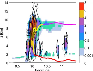
Fig. 10. Online trajectory ascending in a deep convective cloud in the COSMO2.2 simulation over the southern Po Valley in the evening of the 26 July 1987. The colors denote the position of the trajectory relative to the W–E-oriented vertical section at 45◦ (yellow: in the plane; red: further north; magenta: further south). The color shading shows the total hydrometeor content in g kg−1 and the contours indicate vertical velocity (solid: upward motion; dashed: downward motion) at 20:00 UTC, 26 July 1987, which is the model output time step closest to the ascent of the parcel.
are permeable for subgrid-scale motions, which the model does not aim to represent explicitly. If the latter is the objec-tive of a study, then Lagrangian particle models must be used. The differentiation between subgrid-scale processes and the resolved wind is fundamental, although it relates to different scales and processes for different model resolutions.
Despite the challenges associated with the online com-putation of trajectories, this novel possibility for perform-ing Lagrangian studies is supposed to be useful for high-resolution simulations and even mandatory for studying at-mospheric phenomena with short temporal and spatial scales such as orographic flows or deep convection. There the ad-vent of convection-resolving weather and climate predictions in combination with the calculation of online trajectories can lead to novel insight into the evolution of convective weather systems. For instance, as illustrated in Fig. 10, online trajec-tories can capture the rapid ascent in cumulonimbus clouds from the boundary layer to the upper troposphere and even provide enough data points during the ascent to study the in-cloud processes. Whether such trajectories are realistic of course depends to a large degree on the quality of the un-derlying Eulerian model, but such trajectories may also help to validate the Eulerian model in a more process-oriented way. Future studies addressing this verification aspect more closely, probably also employing observational data, will be very helpful in assessing the accuracy of the online trajecto-ries.
Supplementary material related to this article is available online at http://www.geosci-model-dev.net/6/ 1989/2013/gmd-6-1989-2013-supplement.pdf.
Acknowledgements. We thank Hanna Joos and Michael Sprenger for their enthusiasm for this work and for interesting and stimu-lating discussions on many aspects presented in this article, and Axel Seifert for providing the COSMO-model code including the two-moment microphysics scheme. We also thank both referees, Ulrich Blahak and Petra Seibert, for their valuable input, which clearly enhanced the quality of this paper. ETH is acknowledged for providing the computational resources and for funding the work by ETH research grant ETH-38-11-1.
Edited by: V. Grewe
References
Baldauf, M., Seifert, A., Foerstner, J., Majewski, D., Raschen-dorfer, M., and Reinhardt, T.: Operational convective-scale nu-merical weather prediction with the COSMO-model: Descrip-tion and sensitivities, Mon. Weather Rev., 139, 3887–3905, doi:10.1175/MWR-D-10-05013.1, 2011.
Becker, A. and Keuler, K.: Continous four-dimensional source at-tribution for the Berlin area during two days in July 1994. Part I: The new Euler-Lagrange model system LaMM5, Atmos. Env-iron., 35, 5497–5508, 2001.
Bellasio, R., Scarpato, S., Bianconi, R., and Zeppa, P.: APOLLO2, a new long range Lagrangian particle dispersion model and its evaluation against the ETEX tracer release, Atmos. Environ., 57, 244–256, 2012.
Bertò, A., Buzzi, A., and Zardi, D.: Back-tracking water vapour contribution to a precipitation event over Trentino: a case study, Meteorol. Z., 13, 189–200, 2004.
Brabec, M., Wienhold, F. G., Luo, B. P., Vömel, H., Immler, F., Steiner, P., Hausammann, E., Weers, U., and Peter, T.: Particle backscatter and relative humidity measured across cirrus clouds and comparison with microphysical cirrus modelling, Atmos. Chem. Phys., 12, 9135–9148, doi:10.5194/acp-12-9135-2012, 2012.
Brioude, J., Angevine, W. M., McKeen, S. A., and Hsie, E.-Y.: Numerical uncertainty at mesoscale in a Lagrangian model in complex terrain, Geosci. Model Dev., 5, 1127–1136, doi:10.5194/gmd-5-1127-2012, 2012.
Buzzi, A. and Alberoni, P. P.: Analysis and numerical modelling of a frontal passage associated with thunderstorm development over the po valley and the adriatic sea, Meteorol. Atmos. Phys., 48, 205–224, 1992.
Buzzi, A. and Tibaldi, S.: Cyclogenesis in the lee of the Alps: A case study, Q. J. R. Meteorol. Soc., 104, 271–287, 1978. Buzzi, A., Giovanelli, G., Nanni, T., and Tagliazucca, M.: Study of
high ozone concentrations in the troposphere associated with lee cyclogenesis during ALPEX, Contr. Atm. Phys., 57, 380–392, 1984.
changes in cirrus clouds by geoengineering the stratosphere, J. Geophys. Res., 118, 4533–4548, doi:10.1002/jgrd.50388, 2013. Coude-Gaussen, G., Rognon, P., Bergametti, G., Gomes, L.,
Strauss, B., Gros, J. M., and Coustumer, M. N. L.: Saharan dust on Fuerteventura Island (Canaries): Chemical and mineralogi-cal characteristics, air mass trajectories, and probable sources, J. Geophys. Res., 92, 9753–9771, 1987.
Danielsen, E. F.: Trajectories: Isobaric, isentropic and actual, J. Me-teorol., 18, 479–486, 1961.
Djuric, D.: On the accuracy of air trajectory computations, J. Mete-orol., 18, 597–605, 1961.
Doty, K. G. and Perkey, D. J.: Sensitivity of trajectory calcualtions to the temporal frequency of wind data, Mon. Weather Rev., 121, 387–401, 1993.
Draxler, R. R.: Sensitivity of a trajectory model to the spatial and temporal resolution of the meteorological data during CAPTEX, J. Climate Appl. Meteor., 26, 1577–1588, 1987.
Draxler, R. R. and Hess, G. D.: An overview of the HYSPLIT_4 modelling system for trajectories, dispersion, deposition, Aust. Met. Mag., 47, 295–308, 1998.
Drobinski, P., Steinacker, R., Richner, H., Baumann-Stanzer, K., Beffrey, G., Benech, N., Berger, H., Chimani, B., Dabas, A., Dorninger, M., Dürr, B., Flamant, C., Frioude, M., Furger, M., Gröhn, I., Gubser, S., Gutermann, T., Häberli, C., Häller-Scharnhost, E., Jaubert, G., Lothon, M., Mitev, V., Pechinger, U., Ratheiser, M., Ruffieux, D., Seiz, G., Spatzierer, M., Tschannett, S., Vogt, S., Werner, R., and Zängl, G.: Föhn in the Rhine Val-ley during MAP: A review of its multiscale dynamics in complex valley geometry, Q. J. R. Meteorol. Soc., 133, 897–916, 2007. Duffourg, F. and Ducrocq, V.: Origin of the moisture feeding the
Heavy Precipitating Systems over Southeastern France, Nat. Hazards Earth Syst. Sci., 11, 1163–1178, doi:10.5194/nhess-11-1163-2011, 2011.
Eckhardt, S., Stohl, A., Wernli, H., James, P., Forster, C., and Spichtinger, N.: A 15-year climatology of warm conveyor belts, J. Climate, 17, 218–237, 2004.
Fierro, A. O., Simpson, J., LeMone, M. A., Stranka, J. M., and Smull, B. F.: On how hot towers fuel the Hadley cell: An ob-servational and modeling study of line-organized convection in the equatorial trough from TOGA COARE, J. Atmos. Sci., 66, 2730–2746, 2009.
Forrer, J., Rüttimann, R., Schneiter, D., Fischer, A., Buchmann, B., and Hofer, P.: Variability of trace gases at the high-Alpine site Jungfraujoch caused by meteorological transport processes, J. Geophys. Res., 105, 12241–12251, 2000.
Gheusi, F. and Stein, J.: Lagrangian description of airflow using Eulerian passive tracers, Q. J. R. Meteorol. Soc., 128, 337–360, 2002.
Grams, C. M., Jones, S. C., Davis, C. A., Harr, P. A., and Weiss-mann, M.: The impact of Typhoon Jangmi (2008) on the midlat-itude flow. Part I: Upper-level ridgebuilding and modification of the jet, Q. J. R. Meteorol. Soc., doi:10.1002/qj.2091, 2013. Grell, G. A., Knoche, R., Peckham, S. E., and McKeen, S. A.:
On-line versus offOn-line air quality modeling on cloud-resolving scales, Geophys. Res. Lett., 31, L16117, doi:10.1029/2004GL020175, 2004.
Gross, G., Vogel, H., and Wippermann, F.: Dispersion over and around a steep obstacle for varying thermal stratification - nu-merical simulations, Atmos. Environ., 21, 483–490, 1987.
Haag, W. and Kärcher, B.: The impact of aerosols and gravity waves on cirrus clouds at midlatitudes, J. Geophys. Res., 109, D12202, doi:10.1029/2004JD004579, 2004.
Haagenson, P. L., Gao, K., and Kuo, Y.-H.: Evaluation of meteo-rological analyses, simulations, and long-range transport calcu-lations using ANATEX surface tracer data, J. Appl. Meteor., 29, 1268–1283, 1990.
Hoyle, C. R., Luo, B. P., and Peter, T.: The origin of high ice crystal number densities in cirrus clouds, J. Atmos. Sci., 66, 508–518, 2005.
Kahl, J. D.: A cautionary note on the use of air trajectories in inter-preting atmospheric chemistry measurements, Atmos. Environ., 27A, 3037–3038, 1993.
Kärcher, B. and Lohmann, U.: A parameterization of cirrus clouds formation: Homogeneous freezing of supercooled aerosols, J. Geophys. Res., 107, 4010, doi:10.1029/2001JD000470, 2002. Kljun, N., Sprenger, M., and Schär, C.: Frontal modification and lee
cyclogenesis in the Alps: A case study using the ALPEX reanal-ysis data set, Meteorol. Atmos. Phys., 78, 89–105, 2001. Kogan, Y. L.: Large-eddy simulation of air parcels in stratocumulus
clouds: Time scales and spatial variability, J. Atmos. Sci., 63, 952–867, 2006.
Kröner, N.: Accuracy of trajectory calculation: Dependence on the temporal resolution of the input files, Master thesis, ETH Zurich, 2011.
Lefohn, A. S., Wernli, H., Shadwick, D., Limbach, S., Oltmans, S. J., and Shapiro, M.: Importance of stratospheric-tropospheric transport in affecting surface ozone concentrations in the west-ern and northwest-ern tier of the United States, Atmos. Environ., 45, 4845–4857, 2011.
Methven, J., Arnold, S. R., Stohl, A., Evans, M. J., Avery, M., Law, K., Lewis, A. C., Monks, P. S., Parrish, D. D., Reeves, C. E., Schlager, H., Atlas, E., Blake, D. R., Coe, H., Crosier, J., Flocke, F. M., Holloway, J. S., Hopkins, J. R., McQuaid, J., Purvis, R., Rappenglück, B., Singh, H. B., Watson, N. M., Whalley, L. K., and Williams, P. I.: Estabilishing Lagrangian connections be-tween observations within air masses crossing the Atlantic dur-ing the Interational Consortium for Atmospheric Research on Transport and Transformation experiment, J. Geophys. Res., 111, D23S62, doi:10.1029/2006JD007540, 2006.
Miller, J. M.: The use of back air trajectories in interpreting atmo-spheric chemistry data: a review and bibliography, NOAA tech-nical memorandum ERL-ARL-155, Air Resources Laboratory, Silver Spring, MD, 1987.
Paccagnella, T., Tibaldi, S., Buizza, R., and Scoccianti, S.: High-resolution numerical modelling of convective precipitation over northern Italy, Meteorol. Atmos. Phys., 50, 143–163, 1992. Petterssen, S.: Weather analysis and forecasting, McGraw-Hill,
New York, 1940.
Pfahl, S. and Wernli, H.: Air parcel trajectory analysis of stable iso-topes in water vapor in the eastern Mediterranean, J. Geophys. Res., 113, D20104, doi:10.1029/2008JD009839, 2008.
Reap, R. M.: An operational three-dimensional trajectory model, J. Appl. Meteor., 11, 1193–1202, 1972.
Reisinger, L. M. and Mueller, S. F.: Comparison of tetroon and com-puted trajectories, J. Climate Appl. Meteor., 22, 664–672, 1983. Reithmeier, C. and Sausen, R.: ATTILA: atmospheric tracer
Roch, A.: Orographic blocking in the Alps: A climatologic La-grangian study, Master thesis, ETH Zurich, 2011.
Rolph, G. D. and Draxler, R. R.: Sensitivity of three-dimensional trajectories to the spatial and temporal densities of the wind field, J. Appl. Meteor., 29, 1043–1054, 1990.
Rössler, C. E., Paccagnella, T., and Tibaldi, S.: A three-dimensional atmospheric trajectory model: Application to a case study of Alpine lee cyclogenesis, Meteorol. Atmos. Phys., 50, 211–229, 1992.
Scheele, M. P., Siegmund, P. C., and Velthoven, P. F. J.: Sensitivity of trajectories to data resolution and its dependence on the start-ing point: in or outside a tropopause field, Meteorol. Appl., 3, 267–273, 1996.
Seibert, P.: Convergence and accuracy of numerical methods for tra-jectory calculations, J. Appl. Meteor., 32, 558–566, 1993. Seifert, A. and Beheng, K. D.: A two-moment cloud microphysics
parameterization for mixed-phase clouds. Part 1: Model descrip-tion, Meteorol. Atmos. Phys., 92, 45–66, 2006.
Shaw, N. and Lempfert, R. G. K.: The life history of surface air cur-rents, M. O. Memoir, 174, reprinted in Selected Meteorological Papers of Sir Napier Shaw (London, MacDonald and Co., 1955, 15–131), 1906.
Shaw, W. N., Lempfert, R. G. K., and Brodie, F. J.: The meteoro-logical aspects of the storm of February 26–27, 1903, Q. J. R. Meteorol. Soc., 29, 233–264, 1903.
Sodemann, H., Schwierz, C., and Wernli, H.: Interannual variability of Greenland winter precipitation sources: Lagrangian moisture diagnostic and North Atlantic Oscillation influence, J. Geophys. Res., 113, D03107, doi:10.1029/2007JD008503, 2008.
Spichtinger, P. and Krämer, M.: Tropical tropopause ice clouds: a dynamic approach to the mystery of low crystal numbers, At-mos. Chem. Phys., 13, 9801–9818, doi:10.5194/acp-13-9801-2013, 2013.
Sprenger, M. and Wernli, H.: A northern hemispheric climatology of cross-tropopause exchange for the ERA15 time period (1979– 1993), J. Geophys. Res., 108, 8521, doi:10.1029/2002JD002636, 2003.
Steinacker, R.: Airmass and frontal movement around the Alps, Riv. Meteorol. Aeronautica, 43, 85–93, 1984.
Steinacker, R.: Alpiner Föhn - eine neue Strophe zu einem alten Lied, Promet, 32, 3–10, 2006.
Stern, D. P. and Zhang, F.: How does the eye warm? Part II: Sensi-tivity to vertical wind shear, and a trajectory analysis, J. Atmos. Sci., 70, 1849–1873, doi:10.1175/JAS-D-12-0258.1, 2013. Stevens, B., Feingold, G., Cotton, W., and Walko, R. L.: Elements of
the microphysical structure of numerically simulated nonprecip-itating stratocumulus, J. Atmos. Sci., 53, 980–1006, 1996. Stohl, A.: Computation, accuracy and applications of trajectories –
a review and bibliography, Atmos. Environ., 32, 947–966, 1998. Stohl, A. and Koffi, N. E.: Evaluation of trajectories calculated from ECMWF data against constant volume balloon flights dur-ing ETEX, Atmos. Environ., 32, 4151–4156, 1998.
Stohl, A. and Seibert, P.: Accuracy of trajectories as determined from the conservation of meteorological tracers, Q. J. R. Meteo-rol. Soc., 124, 1465–1484, 1998.
Stohl, A., Wotawa, G., Seibert, P., and Kromp-Kolb, H.: Interpola-tion errors in wind fields as a funcInterpola-tion of spatial and temporal resolution and their impact on different types of kinematic tra-jectories, J. Appl. Meteor., 34, 2149–2165, 1995.
Stohl, A., Haimberger, L., Scheele, M. P., and Wernli, H.: An in-tercomparison of results from three trajectory models, Meteorol. Appl., 8, 127–135, 2001.
Stohl, A., Forster, C., Frank, A., Seibert, P., and Wotawa, G.: Technical note: The Lagrangian particle dispersion model FLEXPART version 6.2, Atmos. Chem. Phys., 5, 2461–2474, doi:10.5194/acp-5-2461-2005, 2005.
Uppala, S. M., Kållberg, P. W., Simmons, A. J., Andrae, U., Bech-told, V. D. C., Fiorino, M., Gibson, J. K., Haseler, J., Hernandez, A., Kelly, G. A., Li, X., Onogi, K., Saarinen, S., Sokka, N., Al-lan, R. P., Andersson, E., Arpe, K., Balmaseda, M. A., Beljaars, A. C. M., Berg, L. V. D., Bidlot, J., Bormann, N., Caires, S., Chevallier, F., Dethof, A., Dragosavac, M., Fisher, M., Fuentes, M., Hagemann, S., Hólm, E., Hoskins, B. J., Isaksen, L., Janssen, P. A. E. M., Jenne, R., Mcnally, A. P., Mahfouf, J.-F., Morcrette, J.-J., Rayner, N. A., Saunders, R. W., Simon, P., Sterl, A., Tren-berth, K. E., Untch, A., Vasiljevic, D., Viterbo, P., and Woollen, J.: The ERA-40 re-analysis, Q. J. R. Meteorol. Soc., 131, 2961– 3012, doi:10.1256/qj.04.176, 2005.
van Dop, H., Addis, R., Fraser, G., Girardi, F., Graziani, G., Inoue, Y., Kelly, N., Klug, W., Kulmala, A., Nodop, K., and Pretel, J.: ETEX: A European Tracer Experiment; Observations, dispersion modelling and emergency response, Atmos. Environ., 32, 4089– 4094, 1998.
Wang, Q.-W. and Xue, M.: Convective initiation on 19 July 2002 during IHOP: High-resolution simulations and analysis of the mesoscale structures and convective initiation, J. Geophys. Res., 117, D12107, doi:10.1029.2012JD017552, 2012.
Weil, J. C., Sullivan, P. P., Patton, E. G., and Moeng, C.-H.: Statis-tical variability of dispersion in the convective boundary layer: Ensembles of simulations and observations, Bound.-Lay. Meteo-rol., 145, 185–210, 2012.
Wernli, H. and Davies, H. C.: A Lagrangian-based analysis of ex-tratropical cyclones. I: The method and some applications, Q. J. R. Meteorol. Soc., 123, 467–489, 1997.
Whitaker, J. S., Uccellini, L. W., and Brill, K. F.: A model-based di-agnostic study on the rapid development phase of the Presidents’ Day Cyclone, Mon. Weather Rev., 116, 2337–2365, 1988. Würsch, M.: Lagrangian based analysis of airflow during föhn in
the Alps, Master thesis, ETH Zurich, 2009.
Yamaguchi, T. and Randall, D. A.: Cooling of entrained parcels in a large-eddy simulation, J. Atmos. Sci., 69, 1118–1136, 2012. Yeo, K. and Romps, D. M.: Measurement of convective entrainment