Nonlinear Processes
in Geophysics
c
European Geophysical Society 2001
Lyapunov, Floquet, and singular vectors for baroclinic waves
R. M. Samelson
College of Oceanic and Atmospheric Sciences, 104 Ocean Admin Bldg, Oregon State University, Corvallis, OR, USA Received: 18 September 2000 – Accepted: 29 January 2001
Abstract.The dynamics of the growth of linear disturbances
to a chaotic basic state is analyzed in an asymptotic model of weakly nonlinear, baroclinic wave-mean interaction. In this model, an ordinary differential equation for the wave ampli-tude is coupled to a partial differential equation for the zonal flow correction. The leading Lyapunov vector is nearly par-allel to the leading Floquet vectorφ1of the lowest-order un-stable periodic orbit over most of the attractor. Departures of the Lyapunov vector from this orientation are primarily ro-tations of the vector in an approximate tangent plane to the large-scale attractor structure. Exponential growth and de-cay rates of the Lyapunov vector during individual Poincar´e section returns are an order of magnitude larger than the Lya-punov exponentλ≈0.016. Relatively large deviations of the Lyapunov vector from parallel toφ1are generally associated with relatively large transient decays. The transient growth and decay of the Lyapunov vector is well described by the transient growth and decay of the leading Floquet vectors of the set of unstable periodic orbits associated with the attrac-tor. Each of these vectors is also nearly parallel toφ1. The dynamical splitting of the complete sets of Floquet vectors for the higher-order cycles follows the previous results on the lowest-order cycle, with the vectors divided into wave-dynamical and decaying zonal flow modes. Singular vec-tors and singular values also generally follow this split. The primary difference between the leading Lyapunov and singu-lar vectors is the contribution of decaying, inviscidly-damped wave-dynamical structures to the singular vectors.
1 Introduction
The predictability of geophysical fluid flows is an impor-tant and interesting scientific issue, which combines prac-tical and theoreprac-tical elements. Of particular pracprac-tical inter-est is the problem of numerical weather prediction. One
ap-Correspondence to:R. M. Samelson ([email protected])
proach to this problem involves the use of ensemble fore-casting techniques, which attempt to improve a single at-mospheric forecast by combining multiple model predictions (Epstein, 1969; Leith, 1974).
Recent operational implementations of ensemble fore-casting in global numerical weather prediction models rely on two different methods for ensemble generation: bred modes (Toth and Kalnay, 1997) and singular vectors (Buizza et al., 1993; Ehrendorfer and Tribbia, 1997). Bred modes are obtained by iterating a “breeding” cycle, in which the differences between ensemble members and a control forecast are rescaled and added to the analysis at each anal-ysis cycle to initialize a new ensemble. Singular vectors are optimal disturbances (Lorenz, 1965; Farrell, 1989) that max-imize specific measures of disturbance growth over specific forecast intervals.
The object of the present contribution is to compute and analyze singular vectors and the simplest analogs of bred modes in a simple, physically consistent model of baro-clinic wave-mean interaction, in order to develop insight into the processes of disturbance growth in time-dependent baroclinic flows and their relation to ensemble forecasting methods. The present study shares this general motivation with the closely related study of Samelson (2001; hereafter S2001), which it extends and as a companion to which it should be read, and with many recent studies of systems ranging in complexity from the low-order Lorenz (1963) equations to operational numerical weather prediction mod-els (e.g. Buizza and Palmer, 1995; Buizza, 1995; Trevisan and Legnani, 1995; Legras and Vautard, 1996; Szunyogh et al.,1997; Vannitsem and Nicolis, 1997).
The present study extends S2001, which focused on dis-turbances to stable and unstable time-periodic solutions of the model equations, to consider dirsturbances to ir-regular, chaotic solutions. Since the pioneering work of Lorenz (1963), deterministic chaos has served as an endur-ing metaphor for the observed irregularity and unpredictabil-ity of the atmosphere. One goal of this study is, in a limited way and for one particular physical model, to explore this metaphor quantitatively and concretely, in the context of en-semble forecasting. The approach is partially motivated by recent work on cycle expansions for chaotic systems (e.g. Artuso et al., 1990a, 1990b; Christiansen et al., 1997; Cvi-tanovi´c et al., 2000), and is related to a recent study based on the Lorenz system (Trevisan and Pancotti, 1998).
The model is briefly reviewed in Sect. 2. Section 3 de-scribes the chaotic basic state and its linear instability, and Sects. 4 and 5 discuss the Floquet and singular vector anal-yses, respectively. Section 6 contains the discussion, and Sect. 7 summarizes the results.
2 Model
The model studied here is a two-layer, f-plane, quasi-geostrophic fluid in a periodic channel with a rigid lid at the upper boundary, and Ekman dissipation at both the upper and lower boundaries. Weakly nonlinear baroclinic wave-mean interaction has been studied in this model by Pedlosky (1971) and Pedlosky and Frenzen (1980), and is summarized in Ped-losky (1987). The model equations and the relevant parame-ters are summarized here, with notation primarily following the previous references, to which the reader is referred for additional details.
For a weakly supercritical mean flow, a weakly nonlin-ear disturbance consisting of a single zonal wave component generates a small correction to the mean zonal flow, which, in turn, affects the growth or decay of the wave. The asymp-totic analysis conducted by Pedlosky (1971) yields the cou-pled system of equations describing this interaction. This system consists of a second-order ordinary differential equa-tion for the wave amplitudeA(t ), coupled to a partial differ-ential equation for the mean flow correction9(y, t ). If9 is expanded in terms of sinusoidal cross-channel modes, the partial differential equation transforms into an infinite set of coupled ordinary differential equations, which may be writ-ten as
dA
dt = −γ A+B, (1)
dB dt = −
1
2γ B+A "
1+1 2γ
2−
J
X
j=1
aj(A2+Vj)
# , (2) dVj
dt = −γ (bjVj−cjA
2), j =1,2, ..., (3) whereJ → ∞for the complete expansion, and
aj =
32m2(2j −1)2
(2j−1)2−4m22
(2j −1)2π2+K2, (4)
bj =
(2j −1)2π2
(2j −1)2π2+K2, (5)
cj =2−bj. (6)
Here,K = (k2+m2π2)1/2 is the total wave number of the baroclinic wave, andγ = r/(2σ )is the Ekman damp-ing coefficientεrscaled by twice the inverse time scale, the small exponential growth rate εσ of the linear wave. The relations between A, B, Vj and the upper and lower layer
stream functions are discussed in S2001. Briefly,A is the scaled amplitude of the wave,B is a measure of the phase shift between the upper and lower layers, and eachVj
rep-resents a scaled combination of zonal flow componentj and the squared wave amplitude. Sinceaj ∼ j−4 asj → ∞,
Eqs. (1–3) may be well approximated numerically by trun-cating the sum in Eq. (2) at a finite valueJ, as is done here.
3 Attractor structure and Lyapunov vectors
3.1 Theγ =0.1315 attractor
A numerical exploration of Eqs. (1–3) for a range of pa-rameter values has been conducted by Pedlosky and Frenzen (1980). Following S2001, the present study focuses on a set of solutions withm=1 andK2=2π2(k=π), correspond-ing to a wave with equal zonal and meridional scales, and with friction parameterγ = 0.1315. The results described here were obtained with a truncation at J = 6 in Eq. (2). The differences between the present numerics and those of Pedlosky and Frenzen (1980) lead to small, but inessential differences in the solutions and their dependence onγ. The numerical techniques used in the present study are the same as those described in S2001.
Forγ = 0.1280 (and for a range of adjacentγ), the nu-merical solutions approach a limit cycle (S2001, Figs. 1–3). Note that since the Eqs. (1–3) are unchanged by the trans-formation(A, B) → (−A,−B), an asymmetric solution is accompanied by a twin of opposite parity, corresponding to an arbitrary along-channel phase shift of a half-wavelength. For simplicity, attention is restricted here to the solution with parity such that the maximum value of|A|occurs forA >0. The corresponding results for the twin solutions may be ob-tained by changing the appropriate signs or phases.
1.78 1.8 1.82 1.84 1.86 1.88 1.9 1.92 3.9
3.95 4 4.05 4.1 4.15 4.2 4.25 4.3
A
V 1
(a)
1.780 1.8 1.82 1.84 1.86 1.88 1.9 1.92 100
200 300 400 500 600
A
(b)
Fig. 1. (a)A−V1 phase plane structure of the attractor on the
{B=0, A >0}Poincar´e section, from 25 000 points. The large dot shows the location of the lowest-order unstable periodic orbitp1.
The diamonds show the orientation of the leading Floquet vector of
p1. The 1993 intersection points of the first 157 unstable cycles are
also shown, offset inV1by−0.05. (b)Histogram of theA-values
of the 25 000 attractor points in (a).
B ≈dA/dt over most of the cycle, as is true for the linear modes of instability of the steady zonal flow.
Asγ increases past 0.1280, the system undergoes a se-quence of period-doubling bifurcations. Chaos appears to ensue forγ greater than about 0.1309. Here, we focus on the chaotic numerical solution forγ =0.1315. This is the same value of the friction parameterγ for which S2001 studied the properties of the lowest-order unstable periodic orbit, the continuation toγ =0.1315 of theγ =0.1280 limit cycle. The solution on theγ =0.1315 attractor is generally similar to theγ =0.1280 limit cycle, but with irregular fluctuations in the maximum and minimum amplitude of the oscillation.
The γ =0.1315 attractor is conveniently analyzed by considering the Poincar´e section on the half-plane {B=0, A >0}. A projection on the A−V1 phase plane
of a set of points at which a γ=0.1315 numerical solu-tion intersects this half-plane as shown in Fig. 1a. These points lie nearly along a single curve. The Poincar´e map constructed by plotting theA-values of successive intersec-tions closely approximates a one-dimensional, single hump map that is asymmetric, but otherwise resembles the logistic map (S2001, Fig. 4).
The following analysis focuses entirely on the structure of the attractor as it is represented in this Poincar´e section. An A−Bphase plane projection of the continuousγ =0.1315 attractor time series is shown in Fig. 2b of S2001. The return time between successive Poincar´e section points is approx-imately equal to the period of the lowest-order unstable pe-riodic orbit (24.479), or physically to two weakly nonlinear baroclinic wave life cycles, since each oscillation involves a growth and decay of waves with alternating signs or phases. A histogram of theA-values of the points in Fig. 1a is shown in Fig. 1b, and indicates that, with notable exceptions near the maximum and minimum values ofAand several inter-mediate points, the 25 000 points of the numerical solution are approximately uniformly distributed inA.
3.2 Lyapunov exponent and vectors
The leading Lyapunov exponentλ and Lyapunov vectorv on the attractor were approximated numerically in the stan-dard way (Shimada and Nagashima, 1979; Bennetin et al., 1980): the long-time evolution of an arbitrary, small dis-turbance to the attractor solution was computed using the linearized equations. The amplification of the linear distur-bance on each return to the Poincar´e section was computed (using the standard inner-product norm in the {A, B, Vj}
phase space), and the disturbance was then renormalized each time to prevent unbounded growth. To limit the in-fluence of transients associated with the arbitrary initializa-tion, only the last 25 000 of 50 000 Poincar´e returns are used in the analysis (corresponding to a time series of length ≈25 000×24.479 ≈6×10⁵, or 50 000 weakly nonlinear wave life cycles). Note that this time series is much longer than the length of time over which the numerical solution can track the actual unstable solution from a given initial point with neglible numerical error; it is assumed in the usual way (e.g. a shadowing property) that the numerical results are still meaningful, at least as local and statistical descriptions.
The Lyapunov exponentλwas computed as the mean ex-ponential growth rate of the linearized disturbance. During the last 15 000 returns,λ=0.01608±0.00001, where the er-ror is the standard deviation. For the unstable time-dependent numerical solution on the attractor, this mean exponential growth rate is analogous to the exponential growth rates of normal-mode instabilities of steady flows, as it is the rate at which the fastest growing disturbance will amplify asymp-totically in the long-time limit.
1.780 1.8 1.82 1.84 1.86 1.88 1.9 1.92 0.5
1 1.5
A
arccos(v.phi
1
)
(a)
1.780 1.8 1.82 1.84 1.86 1.88 1.9 1.92 0.05
0.1 0.15 0.2 0.25 0.3
A
arccos(v.v
t
)
(b)
Fig. 2. (a)Relative angles of Lyapunov vectors and the leading Floquet vectorφ1of the lowest-order unstable periodic orbitp1, vs. A. (b) Relative angles of Lyapunov vectors and the approximate tangent plane to the attractor vs.A. Note the change in vertical scale from (a) to (b).
normal modes of linear instability of steady flows. At each point, any disturbance to the time-dependent numerical so-lution that is not orthogonal tov will ultimately grow in-definitely under the linearized dynamics, approaching the structure ofv asymptotically. Over most of the attractor,v is nearly tangent to the large-scale structure of the attractor. This is indicated in Fig. 2a, in which|arccos(v·φ1)|(with the standard inner-product, and unit vectorsvandφ1) is plot-ted versusAfor each Poincar´e intersection point, whereφ1 is the leading Floquet vector of the lowest-order unstable pe-riod orbitp1atγ = 0.1315. The Floquet vectorφ1is, in turn, approximately tangent to the large-scale structure of the attractor, as indicated in Fig. 1a (see also S2001). Figure 2a also indicates that φ1 provides a good approximation of v over most of the attractor. The physical structure of φ1 is shown in Fig. 9b of S2001.
A planar approximation to the large-scale attractor struc-ture at the Poincar´e section can be constructed from the
tan-−0.20 −0.15 −0.1 −0.05 0 0.05 0.1 0.15 0.2 0.1
0.2 0.3 0.4 0.5 0.6 0.7 0.8 0.9 1
Lyapunov/Floquet vector amplif. rate; Floquet exp. (a)
1.78 1.8 1.82 1.84 1.86 1.88 1.9 1.92 −0.2
−0.15 −0.1 −0.05 0 0.05 0.1 0.15
A
Lyapunov vector amplification rate
(b)
Fig. 3. (a)Normalized histograms of Poincar´e return exponential growth ratesλT andλ1T of Lyapunov (thick solid line) and leading Floquet (thin) vectors, respectively, and leading Floquet exponents
λ1 (dashed). (b) Poincar´e return exponential growth ratesλT of Lyapunov vectors vs.A.
gentφ2top1and a linear approximation to the attractor on the section, in which the coordinates{Vj}are parameterized
in terms ofA(for example,V1= −2.1379A+8.0763; com-pare to Fig. 1a). The Lyapunov vectorv is essentially tan-gent to this plane over almost all of the section (Fig. 2b). Most of the large angles betweenv andφ1 arise when the Lyapunov vector rotates away from φ1 but remains within the large-scale tangent plane to the attractor. Thus, the Lya-punov vector does provide, for this relatively simple attractor geometry, a useful guide to the distribution of nearby states on the attractor.
Despite this near uniformity across the attractor of the Lyapunov vector orientation, the individual Poincar´e return growth rates λT, from which the mean growth rateλ was
expo-nents computed in this manner. TheλT are the mean
ex-ponential rates of growth of the Lyapunov vectorv (in the standard norm) during each return to the Poincar´e section, computed according toλT =ln(|v(t+T )|/|v(t )|)/T, prior to renormalization of v(t +T ), whereT ≈ 24 is the re-turn time. TheλT are bimodally distributed, with a broad
peak nearλand a distinct secondary peak near 0.05 (Fig. 3a). Many of theλT are as small as−0.02 or as larger as 0.05;
these variations arise over large parts of the attractor despite the small departures ofvfromφ1(Fig. 3b); for comparison, φ1 has Floquet exponent (see below)λ1 ≈ 0.025, slightly larger thanλ.
Extreme values ofλT occur wherev is the farthest from the tangent toφ1, or the attractor (Figs. 2, 3a, 4a, 4c). All (relatively) large departures ofv from these tangencies are associated with a decay ofv(λT <0); as tangency withφ1 is approached, λT approaches λ1≈0.025 (Fig. 4b). The smallestλT are found nearA=1.826 (Fig. 3b), consistent
with the peak and vanishing slope of the approximate one-dimensional map at this point. Most of the positive val-ues ofλT are found in A <1.81, while mostλT are
nega-tive forA >1.81. Thus, the disturbances described by the Lyapunov vector tend to amplify only when the wave ampli-tudeAis small, and they decay whenAis large or near the critical value of 1.826. This is consistent with the general character of the oscillation, in which nonlinear (largeA) sta-bilizing mechanisms arrest the growth of the linear (smallA) instability.
4 Periodic orbits and Floquet vectors
One approach to the study of the structure and dynamics of chaotic systems involves the analysis of an associated set of unstable periodic orbits (e.g. Cvitanovi´c et al., 2000). This analysis is simplified if a symbolic dynamics can be iden-tified that relates the orbits to symbol sequences. As noted above, in the present case, the evolution forγ =0.1315 may be usefully represented by a one-dimensional map (S2001, Fig. 4). From the spline representation of this map, unstable period orbits were determined in the standard way by asso-ciating the symbols 0 and 1 with the intervals to the left and right, respectively, of the point where the map achieves its maximumA=1.826, generating a set of binary symbol se-quences, and finding the corresponding unique orbit points by inverse iteration. These points were then used as first guesses for the periodic points of the differential equations, which were improved using Newton’s method. The result of this set of calculations is a set of unstable periodic orbits that are related in an essential way to the attractor dynamics and “fill out” (more precisely, and under certain conditions that may or may not strictly hold here, are dense on) the attrac-tor. For some examples of these orbits, see Figs. 5 and 9a of S2001.
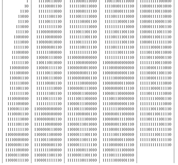
A list of all symbol sequences up to length 15 for which unstable cycles were computed forγ = 0.1315 is given in Table 1. There are a total of 157 such cycles. In the present
0 0.2 0.4 0.6 0.8 1 1.2 1.4 1.6 −0.2
−0.15 −0.1 −0.05 0 0.05 0.1 0.15
arccos(v.phi1)
Lyapunov vector amplification rate
(a)
0 0.01 0.02 0.03 0.04 0.05
−0.2 −0.15 −0.1 −0.05 0 0.05 0.1 0.15
arccos(v.phi
1)
Lyapunov vector amplification rate
(b)
0 0.01 0.02 0.03 0.04 0.05 −0.2
−0.15 −0.1 −0.05 0 0.05 0.1 0.15
arccos(v.v
t)
Lyapunov vector amplification rate
(c)
Fig. 4. (a)Scatter plot of Poincar´e return exponential growth rates
λT vs. relative angles of Lyapunov vectors and the leading Floquet vectorφ1of the lowest-order unstable periodic orbitp1. (b)Same as (a), but with expanded scale for small angles.(c)Scatter plot of Poincar´e return exponential growth ratesλT vs. relative angles of Lyapunov vectors and the approximate tangent plane to the attractor.
1.780 1.8 1.82 1.84 1.86 1.88 1.9 1.92 0.005
0.01 0.015 0.02 0.025
A
Floquet exponent
(a)
1.78 1.8 1.82 1.84 1.86 1.88 1.9 1.92 −0.2
−0.15 −0.1 −0.05 0 0.05 0.1 0.15
A
Floquet vector amplif. rate
(b)
1.780 1.8 1.82 1.84 1.86 1.88 1.9 1.92 0.5
1 1.5
A
arccos(a
1 .phi
1
)
(c)
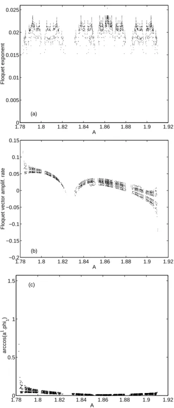
Fig. 5. (a)Floquet exponents for 157 unstable cycles, plotted vs.
Aat each of the 1993 intersection points of the 157 cycles with the Poincar´e section.(b)Poincar´e return exponential growth ratesλ1T of the leading Floquet vector vs. A, for each of the 157 cycles.
(c)Relative angles of the leading Floquet vector for each cycle and the leading Floquet vectorφ1of the lowest-order unstable periodic
orbitp1.
sequence containing 00, since all points in the left-hand inter-val are mapped to points in the right-hand interinter-val. The 1993 points where these 157 cycles intersect the Poincar´e section
are shown in Fig. 1a, withV1 values offset by−0.05. The coverage of the attractor is not uniform, and there are several large gaps, for example, nearA=1.82 andA=1.88.
The solutions of the linearized equations for small distur-bances to these unstable cycles may be computed by standard techniques for linear differential systems with periodic coef-ficients (e.g. Coddington and Levinson, 1955), often known as Floquet theory, as described in detail in S2001. The so-lutions are obtained for the truncationJ = 6, so the result of each of these calculations is a set of 8 time-dependent normal-modes or “Floquet vectors”{φj, j = 1, ...,8}and
8 corresponding Floquet exponents{λj, j = 1, ...,8}; the
λj are the mean exponential growth (or decay) rates of the
corresponding disturbance over the cycle length. Note that the exponentsλj will, in general, differ from cycle to cycle,
but for simplicity, the dependence on cycle is dropped from the notation here. Except for the exponential growth factors, each of these Floquet vectors is also periodic, with the pe-riod equal to the cycle pepe-riod (or twice the cycle pepe-riod). For an example of the physical structure of one of these Floquet vectors, see Fig. 9b of S2001.
The Floquet exponents for these 157 cycles are dis-tributed essentially in same way as those shown in Fig. 8 of S2001: for each cycle, there is one growing mode (λ1 > 0), one neutral mode (λ2 ≈ 0), and six decaying modes (λj < 0, j = 3, ...,8). The neutral (j = 2) and damped
zonal flow (j = 4, ..,7) modes have λj nearly
indepen-dent of cycle, while the values of λ1, λ3, and λ8 fluctu-ate. The distribution ofλ1 for the 157 cycles is shown in Fig. 3a; the maximum and minimum values ofλ1are 0.0253 (for thep1cycle) and 0.0153 (for a 12-cycle with sequence 110111011010).
If the leading Floquet exponentλ1for each cycle is plotted at the Poincar´e section points of the corresponding cycle, the resulting distribution is not smooth (Fig. 5a). The smallest λ1tends to occur at the edges of the gaps in coverage noted above, suggesting the presence of weakly unstable cycles of longer cycle length. This hypothesis is consistent with the relatively small value of the Lyapunov exponentλcomputed above, compared to most of the first 157 leading Floquet ex-ponentsλ1; according to the cycle expansion theory,λshould be accurately approximated by a suitable average of theλ1, weighted inversely by stability.
The leading Floquet vectors of higher-order cycles are, in general, nearly parallel to the leading Floquet vectorφ1of the lowest-order cyclep1(Fig. 5c). Individual Poincar´e return growth ratesλj T of the Floquet vectors were computed in the
same manner as the Lyapunov vector growth ratesλT; they
are the mean exponential growth or decay rates of the corre-sponding Floquet vector during each return to the Poincar´e section. The amplification factorsλ1T of the leading Floquet
vectors show a pattern (Fig. 5b) that is strikingly similar to that of the Lyapunov vector growth ratesλT (Fig. 3b). The
distribution of the λ1T from the first 157 cycles (Fig. 3a)
closely resembles the distribution of theλT; note that it
re-Table 1.Symbol sequences for first 157 unstable cycles forγ =0.1315
1 11110111010 1111010111010 11011101111010 111111111101010
10 11110101110 1111110111010 11110101111110 110101111011010
1110 11111111010 1111010111110 11111010111110 110101110111010
11010 11111101110 1111011111010 11110111111010 110101111111010
11110 11110111110 1111110101110 11111110101110 110101110101110
111010 11111111110 1111111111010 11111111111010 110101111101110
111110 111010101010 1111011101110 11111011101110 110101111011110
1101010 111110101010 1111111101110 11110111101110 110101110111110
1111010 110101011010 1111011111110 11111111101110 110101111111110
1111110 111010101110 1111110111110 11110111111110 111111010111010
11101010 111111101010 1111111111110 11111110111110 111101110111010
11111010 110101111010 11101010101010 11111111111110 111101110101110 11111110 110111011010 11111010101010 110101010101010 111111110111010 110101010 110101111110 11010101011010 111101010101010 111101011111010 111101010 111110111010 11010101011110 110101010101110 111101011101110 110101110 111101111010 11101010101110 111111010101010 111101011111110 111111010 111110101110 11111110101010 110101010111010 111111011111010 111101110 111111111010 11010101111010 110101010111110 111111010111110 111111110 111111101110 11101011101010 110101110101010 111101111111010 1110101010 111101111110 11111011101010 111101110101010 111111110101110 1111101010 111111111110 11010111101010 111101010101110 111111111111010 1101011110 1101010101010 11110111101010 111111110101010 111111011101110 1110101110 1111010101010 11111010101110 110101011101010 111101110111110 1111111010 1101010101110 11111111101010 110101011111010 111101111101110 1111101110 1111110101010 11010111011010 110101011101110 111111111101110 1111111110 1101010111010 11010111111010 111101011101010 111101111111110 11010101010 1101011101010 11010111101110 111111011101010 111111110111110 11110101010 1111011101010 11010111011110 111101010111010 111111011111110 11010101110 1111010101110 11010111111110 111101010111110 111111111111110 11111101010 1111111101010 11111010111010 110101111101010
11010111010 1101011101110 11101011101110 111101111101010 11010111110 1101011111110 11111110111010 111111010101110
quired to describe most of the transient growth and decay of the Lyapunov vector.
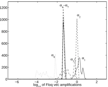
The distribution of the Floquet vector amplificationsαj =
eλj TT generally follows the pattern of the distributions of
Floquet exponentsλj, though with a greatly increased spread
(Fig. 6). Modes 2 and 4–7 have narrow amplification distri-butions, as do their exponents, while modes 1, 3 and 8 have broad distributions. This is consistent with the observation in S2001 that the dynamical splitting between wave-dynamical and damped zonal flow modes observed in the lowest-order cycles persists in the higher-order cycles, and further sug-gests that it persists even during transient growth and decay segments of the higher-order cycles.
5 Singular vectors
The Lyapunov vector, described above, describes the charac-teristic structure of disturbances that amplify indefinitely un-der the linear dynamics, in a way that is analogous to normal-mode instability for steady flows. However, it generally does not describe the linear disturbances that are maximally am-plified after a fixed interval of time. Such optimal
distur-bances, referred to here as singular vectors (SVs), generally exhibit transient growth, and do not have fixed modal struc-ture (e.g. Lorenz, 1965; Farrell, 1989). In this section, SVs are computed on the 157 unstable cycles discussed in the pre-vious section. As shown above, the leading Floquet vectors from these 157 cycles are sufficient to represent much of the detailed time-evolution of the Lyapunov vector over most of the attractor. It is presumed here that SVs based on the com-plete set of Floquet vectors from these 157 cycles are suf-ficient to describe the general characteristics of SVs on the attractor in a similar way.
Consistent with the preceding analysis, SVs are computed here for a single optimization interval (slightly different in duration for each cycle), corresponding to the first Poincar´e return from each Poincar´e section point on each cycle. This is the same set of intervals that was used above to calculate the Lyapunov and Floquet vector transient growth ratesλT
andλj T. The standard inner-product norm in the{A, B, Vj}
−6 −4 −2 0 2 0
200 400 600 800 1000 1200
α1
α2
α3
α4−α7
α8
log
10 of Floq vec amplifications
Fig. 6. Histogram of the base-10 logarithm of the Poincar´e return amplificationαj =eλj TTof Floquet vectorj, j=1, ...,8 for each intersection point of each cycle.
The SVs are otherwise computed in each case in exactly the same manner as in S2001.
The distributions of the singular valuesµj, j =1, ...,8 for
each of the 1993 sets of 8 SVs is shown in Fig. 7. Only the first SV is strongly amplifying. The second is approximately neutral in most cases, the third is mostly decaying, and the fourth through eighth are always decaying. In general, these singular values are consistent with those computed for the lowest-order orbitp1in S2001. The first SV amplifies more rapidly than the first Floquet vector, and the eighth SV de-cays more rapidly than the eighth Floquet vector, while the intermediate SV decay rates follow the corresponding Flo-quet decay rates closely.
The decompositions of the 1993 leading SVs in terms of the Floquet vectors for the corresponding cycle also show a qualitatively similar pattern to that found in S2001 for the lowest-order orbit (Fig. 8). The leading SVs are dominated by the wave-dynamical modes (j =1,2,8), with some con-tribution from the intermediate (j = 3) mode. The projec-tions of the leading SVs on the decaying zonal mean modes (j =4, ...,7) are uniformly small.
6 Discussion
The present analysis of disturbance growth for weakly non-linear baroclinic waves extends a recent study (S2001), which considered only simple, stable and unstable time-periodic basic states, to the case of a chaotic basic state. De-spite the qualitative difference in the time-dependence of the underlying basic states, the present results are largely consis-tent with the results of S2001.
The Lyapunov vector and exponent are the natural concep-tual extensions to the chaotic basic state of the normal modes
−6 −4 −2 0 2
0 200 400 600 800 1000 1200 1400
µ1
µ2
µ3
µ4−µ7
µ8
log
10 of singular values
Fig. 7. Histogram of the base-10 logarithm of the Poincar´e return singular valueµj for singular vectorj, j =1, ...,8 for each inter-section point of each cycle.
and growth rates of linear instabilities of steady basic states, and of the time-dependent Floquet normal modes and growth rates of linear instabilities of time-periodic basic states. For the chaotic basic state, the Lyapunov vector is also the sim-plest analog to the bred modes of numerical bred modes of numerical weather prediction. Over most of the attractor, the Lyapunov vector closely resembles the unstable Floquet nor-mal modeφ1ofp1, the lowest-order unstable periodic orbit analyzed in S2001. In turn, φ1closely resembles the neu-tral modeφ2that is tangent top1, the basic-state oscillation (S2001). Thus, as in S2001, disturbance growth is dominated by the same baroclinic wave processes that control the evo-lution of the basic state. The Lyapunov exponentλ≈0.016 is of the same order but smaller than the leading Floquet ex-ponentλ1≈0.025 ofp1.
Transient growth and decay of the Lyapunov vector occurs on the baroclinic wave time scale with exponential rates that are an order of magnitude larger thanλ. These events involve only minor changes in the structure of the Lyapunov vector, which remains nearly parallel toφ1over most of the attrac-tor. They are accurately represented by the corresponding transient growth and decay of the leading Floquet vectors of the higher-order unstable cycles. Thus, even for these tran-sient events, only the growing modes of the unstable cycles are essentially sufficient to describe the structure and evolu-tion of the Lyapunov vector.
0 0.2 0.4 0.6 0.8 1 0
100 200 300 400 500 600 700 800 900
a1
1
a1
8
a1
2
a1
3
a1
4−a
1 7
Magnitude of Floquet vector component of SV 1
Fig. 8.Histogram of the magnitudes of the Floquet vector compo-nentsa1j, j=1, ...,8 of the leading Poincar´e return singular vector
a1for each intersection point of each cycle.
corresponding maximum transient amplifications of the Flo-quet modes of the unstable cycles, but there is typically only one amplifying singular vector, corresponding to the single amplifying Floquet mode. This is true despite that the opti-mization interval was much shorter than the periods of many of the higher-order cycles.
These results demonstrate that singular vectors and the ex-tensions of normal-mode instabilities for this irregular, time-dependent flow are closely related, as they were found to be in S2001 for the time-periodic basic states. The Lya-punov vector, the simplest analog of bred modes, captures the same disturbance structures and transient growth and de-cay events that dominate the singular vectors, with one im-portant exception: the decaying, inviscidly-damped, wave-dynamical Floquet vector is a central element of the grow-ing sgrow-ingular vectors, but is essentially absent from the Lya-punov vector. The structure of the decaying wave-dynamical mode generally resembles that of the other wave-dynamical modes, which results in a tendency toward non-orthogonality that the singular vector exploits to produce a large transient amplification. Evidently, the damped zonal flow modes are sufficiently different in structure from the wave-dynamical modes that they have a negligible contribution to the grow-ing sgrow-ingular vectors.
It is perhaps surprising that the leading Lyapunov and Flo-quet vectors, here and in S2001, have a structure similar to the tangent to the evolving basic-state flow. As noted above, this indicates that the processes that control distur-bance growth in this model are essentially the same as those that control the evolution of the basic state. In a more com-plex model that admits a wider range of scales and physical processes, or in a similar model but farther from marginal stability of the basic cycle, the similarity between the
unsta-ble modes and the tangent to the flow may not persist. Thus, and in general, the degree to which the present results will extend to more complex models is uncertain.
The present results are generally consistent with the anal-ysis by Trevisan and Pancotti (1998) of Lyapunov, Floquet, and singular vectors for a low-order unstable periodic cycle of the three-component Lorenz (1963) model. Those authors also find that the unstable Floquet mode tends to resemble the tangent along the cycle. Presumably, this would also be true for the higher order cycles of the Lorenz model, as it is here. They also find, as here, that rapidly amplifying singu-lar vectors arise as a consequence of non-orthogonality of the Floquet modes.
7 Summary
This study has addressed the mechanisms of growth of lin-ear disturbances to an irregular, chaotic basic state in a sim-ple model of weakly nonlinear baroclinic wave-mean inter-action. It extends the previous results of S2001, which con-sidered disturbances to time-periodic basic states of the same model. Many of the present conclusions are similar to those of S2001. Disturbance growth in this simple model was found to be related to the wave growth and decay mecha-nisms associated with the time-dependent basic state. Flo-quet vectors of the higher-order unstable cycles were found to divide into two dynamical classes, the first associated with baroclinic wave dynamics and the second with the frictional decay of high meridional modes of the zonal flow. The decompositions of the leading singular vector in terms of the time-dependent Floquet vectors of the higher-order cy-cles generally reflected this dynamical split, with the wave-dynamical components dominating.
In addition, the Lyapunov vector, which for the chaotic basic state in this model is the simplest analog of the bred modes used in numerical weather prediction, was shown to capture most of the transient variability of the growing wave-dynamical Floquet vectors. Since these, along with the tan-gent to the orbit itself, are two of the three dominant com-ponents of the singular vectors, the present results suggest a close relation between bred modes and singular vectors. The primary difference between the two sets of modes is the con-tribution of the decaying wave-dynamical mode to the singu-lar vectors. This confirms one of the hypotheses of S2001 for the nonperiodic state in this simple model. If this re-sult extends to more complex models, and the presence of decaying wave-dynamical modes are found generally to dis-tinguish singular vectors from bred modes, then a practical question that arises in comparing ensemble generation meth-ods is, are the additional decaying wave-dynamical modes valuable to ensemble generation in operational forecasting implementations?
Acknowledgement. This research was supported by the Office of
1997 Summer School on Geophysical Fluid Dynamics at the Woods Hole Oceanographic Institution.
References
Artuso, R., Aurell, E., and Cvitanovi´c, P.: Recycling of strange sets I: Cycle expansions, Nonlinearity, 3, 325–359, 1990a.
Artuso, R., Aurell, E., and Cvitanovi´c, P.: Recycling of strange sets II: applications, Nonlinearity, 3, 361–386, 1990b.
Bennetin, G., Galgani, L., Giorgilli, A., and Strelcyn, J.-M.: Lya-punov characteristic exponents for smooth dynamical systems and for Hamiltonian systems: A method for computing all of them, Meccanica, 15, 9–21 1980.
Buizza, R.: The impact of orographic forcing on barotropic unstable singular vectors, J. Atmos. Sci., 52, 1457–1472, 1995.
Buizza, R. and Palmer, T.: The singular vector structure of the at-mospheric general circulation, J. Atmos. Sci., 52, 1434–1456, 1995.
Buizza, R., Tribbia, J., Molteni, F., and Palmer, T.: Computation of unstable structures for a numerical weather prediction model, Tellus, 45A, 388–407, 1993.
Christiansen, F., Cvitanovi´c, P., and Putkaradze, V.: Spatio-temporal chaos in terms of unstable recurrent patterns, Nonlin-earity, 10, 55–70, 1997.
Coddington, E. and Levinson, N.: Theory of Ordinary Differential Equations, McGraw-Hill, New York, 1955.
Cvitanovi´c, P., Artuso, R., Mainieri, R., and Vatay, G.: Classical and Quantum Chaos, http://www.nbi.dk/ChaosBook/, Niels Bohr Institute, Copenhagen, 2000.
Ehrendorfer, M. and Tribbia, J.: Optimal prediction of forecast error covariances through singular vectors, J. Atmos. Sci., 54, 286– 313, 1997.
Epstein, E.: Stochastic dynamic prediction, Tellus, 21, 739–759, 1969.
Farrell, B.: Optimal excitation of baroclinic waves. J. Atmos. Sci., 46, 1193–1206, 1989.
Klein, P. and Pedlosky, J.: A numerical study of baroclinic instabil-ity at large supercriticalinstabil-ity, J. Atmos. Sci., 43, 1243–1262, 1986. Legras, B. and Vautard, R.: A guide to Lyapunov vectors. Proceed-ings 1995 ECMWF Seminar on Predictability, Vol. I, 143–156, 1996.
Leith, C.: Theoretical skill of Monte Carlo forecasts, Mon. Wea. Rev., 102, 409–418, 1974.
Lorenz, E.: Deterministic nonperiodic flow, J. Atmos. Sci., 12, 130– 141, 1963.
Lorenz, E.: A study of the predictability of a 28-variable atmo-spheric model, Tellus, 17, 321–333, 1965.
Pedlosky, J.: Finite-amplitude baroclinic waves with small dissipa-tion, J. Atmos. Sci., 28, 587–597, 1971.
Pedlosky, J.: Geophysical Fluid Dynamics, Springer-Verlag, New York, 1987.
Pedlosky, J. and Frenzen, C.: Chaotic and periodic behaviour of finite-amplitude baroclinic waves, J. Atmos. Sci., 37, 1177– 1196, 1980.
Samelson, R.: Periodic orbits and disturbance growth for baroclinic waves, J. Atmos. Sci., 58, 436–450, 2001.
Shimada, I. and Nagashima, T.: A numerical approach to ergodic problem of dissipative dynamical systems, Prog. Theor. Phys.,61, 1605–1616, 1979.
Szunyogh, I., Kalnay, E., and Toth, Z.: A comparison of Lyapunov and optimal vectors in a low resolution GCM, Tellus, 49A, 200– 227, 1997.
Toth, Z. and Kalnay, E.: Ensemble forecasting at NCEP and the breeding method, Mon. Wea. Rev., 125, 3297–3319, 1997. Trevisan, A. and Legnani, R.: Transient error growth and local
pre-dictability: a study in the Lorenz system, Tellus, 47A, 103–117, 1995.
Trevisan, A. and Pancotti, F.: Periodic orbits, Lyapunov vectors, and singular vectors in the Lorenz system, J. Atmos. Sci., 55, 390–398, 1998.