www.atmos-chem-phys.net/11/5045/2011/ doi:10.5194/acp-11-5045-2011
© Author(s) 2011. CC Attribution 3.0 License.
Chemistry
and Physics
Middle atmosphere response to the solar cycle in irradiance and
ionizing particle precipitation
K. Semeniuk1, V. I. Fomichev1, J. C. McConnell1, C. Fu2, S. M. L. Melo2, and I. G. Usoskin3
1Department of Earth and Space Science and Engineering, York University, Toronto, Ontario, Canada 2Canadian Space Agency, St.-Hubert, Quebec, Canada
3Sodankyl¨a Geophysical Laboratory, University of Oulu, Oulu, Finland
Received: 5 October 2010 – Published in Atmos. Chem. Phys. Discuss.: 25 October 2010 Revised: 29 April 2011 – Accepted: 11 May 2011 – Published: 31 May 2011
Abstract. The impact of NOxand HOxproduction by three
types of energetic particle precipitation (EPP), auroral zone medium and high energy electrons, solar proton events and galactic cosmic rays on the middle atmosphere is examined using a chemistry climate model. This process study uses en-semble simulations forced by transient EPP derived from ob-servations with one-year repeating sea surface temperatures and fixed chemical boundary conditions for cases with and without solar cycle in irradiance. Our model results show a wintertime polar stratosphere ozone reduction of between 3 and 10 % in agreement with previous studies. EPP is found to modulate the radiative solar cycle effect in the middle atmo-sphere in a significant way, bringing temperature and ozone variations closer to observed patterns. The Southern Hemi-sphere polar vortex undergoes an intensification from solar minimum to solar maximum instead of a weakening. This changes the solar cycle variation of the Brewer-Dobson cir-culation, with a weakening during solar maxima compared to solar minima. In response, the tropical tropopause tempera-ture manifests a statistically significant solar cycle variation resulting in about 4 % more water vapour transported into the lower tropical stratosphere during solar maxima compared to solar minima. This has implications for surface temperature variation due to the associated change in radiative forcing.
Correspondence to:K. Semeniuk ([email protected])
1 Introduction
Although the field of research on the influence of the vari-ability of solar radiation and particle flux on the atmosphere is fast growing, great uncertainty remains concerning im-pacts and the mechanisms involved. Traditionally, model-ing studies of solar variability effects on the climate system have focused on two basic ideas: (1) direct forcing of the troposphere by surface warming associated with changes in the total solar irradiance (TSI) or, in a more complex sce-nario, modulation of the atmosphere-ocean interactions pro-ducing internal oscillations (see for example White et al., 1997; White, 2006); and (2) forcing of the stratosphere asso-ciated with changes in ultraviolet (UV) radiation causing an increase in ozone and associated warming during solar maxi-mum conditions. The latter results in changes in the latitudi-nal distribution of UV heating in the stratosphere which mod-ifies the Eliassen-Palm flux divergence leading to a reduc-tion of the Brewer-Dobson circulareduc-tion (Kodera and Kuroda, 2002; Kuroda and Kodera, 2002; Kodera and Shibata, 2006). Both (1) and (2) operate at the same time increasing the com-plexity of the system response. An extensive model based analysis exploring the different effects and its implications is provided by Rind et al. (2008), which clearly demonstrates our current lack of understanding of the details of how each mechanism operates individually and the impacts of coupled processes. Indeed, Kodera et al. (2008) find that CO2
Recently, more attention has been devoted to the effects of upper atmosphere NOxand HOxproduced from
ioniza-tion by energetic particle precipitaioniza-tion (EPP) on stratospheric ozone. As with UV irradiance, the EPP component of the solar cycle has the potential to influence the tropospheric re-sponse through dynamical processes in the stratosphere that are sensitive to the ozone distribution (Callis et al., 2001; Shindell et al., 1999). Indeed, Sepp¨al¨a et al. (2009) find a statistically significant correlation of wintertime polar north-ern hemisphere surface air temperatures and the Ap index using ERA-40 reanalyses from 1957 to 2002 and ECMWF operational data for subsequent years.
Ionization by energetic particle precipitation in the atmo-sphere is an ubiquitous feature of the Sun-Earth system. The work by Warneck (1972), Swider and Keneshea (1973) and Crutzen et al. (1975) pioneered research into influence of energetic particle precipitation on the chemistry of the at-mosphere through the enhancement of NOx. Following this
early work, Solomon and Crutzen (1981) and Solomon et al. (1981, 1983) pointed out a coupling mechanism whereby thermospheric NOxcould affect the stratosphere. The
Halo-gen Occultation Experiment (HALOE) instrument on the Upper Atmosphere Research Satellite (UARS), and the sub-sequent Atmospheric Trace Molecule Spectroscopy (AT-MOS) and Polar Ozone and Aerosol Measurement (POAM) experiments provided observational evidence for EPP asso-ciated NOxenhancement (Callis et al., 1996; Randall et al.,
1998, 2001; Rinsland et al., 1996; Russell et al., 1984). How-ever, little effort was devoted to the inclusion of EPP ef-fects in chemistry climate models partly due to complex-ity and since they were considered to be of secondary im-portance on climate timescales. This has changed in recent years prompted by conclusive observational evidence of sig-nificant NOx enhancement in the polar regions, extending
to stratospheric altitudes, during major solar proton events (e.g., Siskind, 2000; Randall et al., 2001, 2005; Hauchecorne et al., 2005, 2007; Jackman et al., 2005; L´opez-Puertas et al., 2005). A number of 1, 2 and 3-dimensional model studies, mostly focused on a particular event and sometimes using measured NOx enhancement to force the model have been
conducted since then (for a literature review see Jackman et al., 2008; Reddmann et al., 2010).
The work of Callis et al. (2001) demonstrates that SPEs are not the only type of EPP that can have a significant impact on ozone in the stratosphere and that auroral zone electron precipitation also needs to be taken into account.
The main difficulty in implementing energetic particle pre-cipitation forcing in general circulation models is the com-plexity of the D region ion chemistry. One feasible option is to use parameterizations, relating ionization rates to the pro-duction of NOxand HOx(e.g., Jackman et al., 2008). The
inclusion of ionization by energetic particles in global self-consistent chemistry climate models started with the work of Langematz et al. (2005) and Rozanov et al. (2005), and has varied from from one model to another. For
exam-ple, while the WACCM implementation described by Marsh et al. (2007) includes thermospheric NOxchemistry
explic-itly, it does not account for stratospheric production of NOx
and HOxdue to penetration of high energy galactic cosmic
ray particles (GCR). The implementation in the HAMMO-NIA model, as described in Schmidt et al. (2006), includes stratospheric NO production by galactic cosmic rays follow-ing Heaps (1978) and has the thermospheric NO production based on the scheme of Huang et al. (1998), with the parame-ters adjusted to reproduce the Student Nitric Oxide Explorer (SNOE) satellite instrument measurements (Barth et al., 2003). In the recent EPP studies using the ECHAM5/MESSy chemistry climate model (CCM) low energy electron precip-itation is parameterized in terms of the Ap index and ioniza-tion by solar proton events (SPEs) is included in a compre-hensive way via an online model (Baumgaertner et al., 2009, 2010).
HOxis relatively short-lived (of the order of days) leading
mostly to local effects, while NOxcan lead to both short and
long term (order of months) catalytic ozone destruction in the middle atmosphere. A comprehensive study of the short, middle and long term effects of large SPEs in the polar re-gions has been conducted by Jackman et al. (2008, 2009) involving model and measurements. Ozone destruction in the stratosphere can exceed 10 % and last up to 5 months de-pending of the magnitude of the event. Based on their work it is apparent that CCMs are not able to reproduce all the fea-tures found by satellite measurements of atmospheric com-position. The reasons for this include the fact that CCMs are not constrained to reproduce the observed meteorology and that there is uncertainty about the ion and neutral chemistry.
The multi-model studies of solar variability effects de-scribed by Austin et al. (2008) and the more recent CCMVal-2 project (Manzini et al., CCMVal-2010) noted an improvement of CCMs in the tropical stratosphere ozone response to the solar cycle in irradiance compared to observations. It was hypoth-esized that the improvement could have resulted from either the use of observed varying sea surface temperature (SST) or use of the full cycle in solar irradiance instead of steady solar maximum or minimum conditions. However, there are still unresolved issues such as the much weaker temperature vari-ation in the tropical stratosphere around and below 10 hPa in most models. The CCMVal projects did not investigate the role of EPP and it remains unclear what direct and indirect role it plays. In spite of the conclusions of Gray et al. (2010), we believe more process oriented model studies are neces-sary to understand the effects of EPP. The solar cycle signal is weak and is difficult to extract over short periods, such as the UARS record, from the internal variability of the chaotic ocean-atmosphere system.
atmosphere in a chemistry climate model. Previous studies had fixed solar maximum and minimum conditions (Schmidt et al., 2006) or did not include GCR (Marsh et al., 2007). The modulation of the solar irradiance cycle impact on the stratosphere by EPP is the focus of the work presented here. We conduct pseudo-timeslice ensemble simulations, which include the solar cycle irradiance variation alone and those that also include EPP, using the Canadian Middle At-mosphere Model (CMAM). CMAM is a chemistry climate model which has been modified to include the solar irradi-ance cycle in the solar heating and photolysis rates as de-scribed below. The version of the model used here has a lid at 95 km and does not have a proper thermosphere. As a result, the thermospheric NOxsource is not simulated and
only partially captured by the constant upper boundary con-dition. However, this is a process study intended to assess the impact of EPP on CCMs, which typically lack EPP and do not represent the thermosphere (SPARC CCMVal, 2010). Three types of EPP are active in the model domain and were included: auroral zone medium and high energy electrons, SPEs and GCR. Medium and high energy electrons are found to be sufficient to produce NOxconcentrations in the
meso-sphere similar to solar minimum conditions, which is a very large increase above the regular model state.
In this study we also deliberately do not allow for interan-nual SST variation to reduce the uncertainty in the response. A significant part of the interdecadal variability in climate model simulations originates from the low frequency varia-tion of ocean temperatures. In this study we hope to reduce any aliasing of SST variability onto the solar cycle signal. Also, the solar cycle signal in SSTs is weak and not statisti-cally significant (e.g. Roy and Haigh, 2010) so it is not self-evident that indirect EPP effects play a secondary role com-pared to solar variation of SSTs in the stratospheric response in regions such as the tropics where EPP is small. However, it should be recognized that the comparison of the results of this study with observations is limited since not all processes are included.
The EPP effect on the model chemistry can, to first order, be expressed by the amount of energy deposition, and hence ionization, which results in generation of NOx(Porter et al.,
1976) and HOx(Solomon and Crutzen, 1981). For auroral
zone electrons and SPEs, the vertical profile of the energy deposition is inferred from electron and proton fluxes, ob-served in low earth orbit and in geostationary orbit, respec-tively. For GCR we use the Usoskin and Kovaltsov (2006) parameterization for ionization, which is also based on ob-servations. More details of the model and EPP parameteriza-tions are given in the next section.
2 Description of the model and simulations
The CMAM version used here has a spectral dynamical core with a triangular truncation of 31 spherical harmonics. There are 71 sigma-pressure hybrid levels extending from the
sur-face to about 95 km. A non-zonal sponge layer is applied in the upper two pressure scale heights of the model. The radia-tion scheme of the model takes into account processes which are essential in both the troposphere and middle atmosphere. CMAM is the middle atmosphere version of the CCCma third generation climate GCM, which includes a comprehen-sive set of physical processes, including an interactive land surface scheme, deep and shallow convection parameteriza-tions, orographic and non-orographic gravity wave drag pa-rameterizations. A more detailed description of the CMAM model and its climatology is given in Scinocca et al. (2008), Beagley et al. (1997) and Fomichev et al. (2004).
The model has a comprehensive middle atmosphere photo-chemical scheme as well as heterogeneous chemistry on ice and supersaturated ternary solution (STS) polar stratospheric clouds (PSCs) (de Grandpr´e et al., 1997, 2000) which can capture NOx and HOxproduction and decay, as well as
in-teraction with chlorine and bromine chemistry (Melo et al., 2008; Brohede et al., 2008). The heterogeneous chemistry scheme does not include processing on nitric acid trihydrate (NAT) particles as well as the associated denitrification. This is not considered to be a major omission as activation of chlo-rine on NAT is much less effective than on STS and ice, and denitrification typically contributes less than 30 % to ozone loss (see Hitchcock et al., 2009, and references therein). Red-dmann et al. (2010) found that NAT was enhanced by about 5 % in the Antarctic winter of 2004 and Arctic winter of 2004–2005 when there was significant NOx production by
auroral zone electrons and SPEs. Some underestimation of ozone loss in early spring in response to EPP is expected due to lack of NAT, which typically forms below 25 km. How-ever, as shown in subsequent sections, NOx produced by
EPP can destroy ozone over most altitudes in the polar strato-sphere and at different times of the year depending on EPP type. So the lack of NAT in the model has a secondary impact on the results.
Intrusions of NOx into the stratosphere are observed to
produce a significant enhancement of HNO3(Orsolini et al.,
2005). The mechanisms by which this occurs are not clear and may be any combination of ion-ion, water ion cluster and heterogeneous reactions on aerosols including possibly sul-fate nucleating on meteor smoke (Megner, 2007). For a dis-cussion see Stiller et al. (2005). Since there is no ion chem-istry and the sulfate aerosol surface area density is negligi-ble above 30 km in CMAM, conversion of N2O5into HNO3
in the upper stratosphere winter polar region is underesti-mated. So our simulations do not produce the strong sec-ondary HNO3maximum in the wake of SPEs or large auroral
zone NOxintrusions such as observed in February 2004 (e.g,
Reddmann et al., 2010). Since HNO3is a reservoir species
for both HOxand NOx, there may be some overestimation
of ozone loss through gas phase catalytic cycles in the upper stratosphere.
organic compounds and wet or dry aerosols. Removal of species is by dry deposition at the surface. There is con-vective transport of tracers but without wet removal. Sur-face and lightning emissions of NOx are absent.
Never-theless, the tropospheric ozone values in the model do not deviate significantly from observations (de Grandpr´e et al., 2000). It should be noted that the ozone balance in the tropo-sphere is largely determined by ozone transported from the stratosphere (∼500 Mt yr−1) and photochemical net produc-tion (∼500 Mt yr−1) with loss to surface deposition. Surface emissions and lightning emissions of NOx are∼40 Mt yr−1
and∼5 Mt yr−1, respectively (Lamarque et al., 1996). Given that the model ozone in the troposphere is within 10 % of observations any radiative impact on the dynamics and trans-port is limited. This is borne out by the reasonable climate and sensitivity of the model (Eyring et al., 2006; Karpechko et al., 2010). Neither the lack of wet removal nor additional air quality chemistry in the model should change the fact that GCR leads to a net increase of tropospheric NOyand ozone.
However, in this study this increase is overestimated due to lack of wet removal. Any effect of GCR on cloud formation is not included as this is at best a weak effect (e.g., Pall´e et al., 2004) and another source of uncertainty to be minimized.
Major sudden stratospheric warming (SSW) events are im-portant for NOxtransport from the upper mesosphere to the
stratosphere in the NH due to the associated intensification of the polar vortex in the mesosphere resulting in more ef-fective polar night confinement (Hauchecorne et al., 2007; Semeniuk et al., 2008; Randall et al., 2009). We used the NAM index method described in McLandress and Shepherd (2009) to determine the SSW frequency for the runs pre-sented here. They are found to occur 50±5 % of the time. However, major SSWs in the model have highly variable fea-tures in different years and are not always effective at orga-nizing NOxtransport to the stratosphere. In addition, the
ma-jor SSWs in the model exhibit highly variable clustering and often occur in successive years as opposed to every other year thereby producing multi-year gaps in occurrence. It should be noted that free running model SSWs do not occur at the same time as in observations and there is long term varia-tion of SSW frequency in observavaria-tions as well (Charlton and Polvani, 2007). Analysis of the impact of EPP on the fre-quency of occurrence of SSWs and their transport character-istics will be presented in a subsequent paper.
For the simulations conducted for this study SSTs, sea ice and chemical boundary conditions were specified to be repeated 1979 values for the IPCC SRES A1B greenhouse gas (IPCC, 2000) and the WMO Ab halogen (WMO/UNEP, 2003) scenarios. The SSTs and sea ice were taken from one of the ensemble members of the IPCC AR4 simulations using the coupled ocean-atmosphere version of the CCCma GCM on which CMAM is based. These IPCC AR4 simulations were conducted for the SRES A1B scenario.
The choice of 1979 conditions for halogens leads to the absence of a deep chemical ozone hole. However, the im-pact of this on the results presented here is limited. For 1979 conditions there is a dynamical ozone “hole” in the SH polar region in both the observations and the model. The annual mean total column ozone in the SH polar region exhibits a distinct minimum of about 285 DU in the ground based ob-servations (Fioletov et al., 2002) and 250 DU in the model. A maximum of about 340 DU occurs at 55◦S. This struc-ture persists from year to year in the model and observations, except that in the case of the latter the increasing halogen burden lowers the total column ozone amount globally. The deep dynamical “hole” in the model is partly a consequence of the late break up of the SH polar vortex. The presence of a chemical ozone hole does not significantly change the in-tensity of SH polar vortex and the transport characteristics in this region. Hence, the sensitivity to EPP investigated here should be relevant for models which have varying chlorine.
Since the NOx and HOx produced by EPP reacts with
ClOxto form reservoir species such as ClONO2and HOCl,
there will be reduced gas phase ozone loss through reactive nitrogen, hydrogen and chlorine catalytic cycles under condi-tions of increased chlorine which has been the case following 1979. However, during polar night conditions, ClOxamounts
are very low above the PSC region where most of the effect of EPP on ozone occurs (e.g. Vogel et al., 2008).
To investigate the impact of individual EPP types single realization runs without solar cycle irradiance variation were conducted over the 1979 through 2006 period for auroral zone electrons, SPEs, GCR and a reference case without EPP. The results are presented in Sect. 4. To address dynami-cal variability effects, a three-member ensemble simulation without the solar irradiance cycle but with all three EPP types included was produced and is also presented in Sect. 4. Sec-tion 5 presents analysis of the role of EPP in the 11-yr solar cycle impact on the middle atmosphere using ensemble sim-ulations. A three-member ensemble simulation from 1979 through 2006 without EPP but with the solar irradiance cycle is taken as the reference. A three-member ensemble simu-lation over the same period but with all three types of EPP included together with the solar irradiance cycle is taken as the perturbation. Effects on the long term mean state as well as variation with the solar cycle are considered. The various model experiments are summarized in Table 1.
2.1 Solar irradiance scheme
Table 1.Brief description of the simulations.
Run Ensemble EPP Solar
(1979–2006) members type cycle
Reference 3 none no
Auroral Zone 1 Electrons no
SPEs 1 SPEs no
GCR 1 GCR no
Combined 3 Electrons+SPEs+GCR no
Solar 3 none yes
Solar Combined 3 Electrons+SPEs+GCR yes
in ozone absorption bands between 200 and 300 nm and ex-ceeding 10 % in the molecular oxygen bands at wavelengths shorter than 200 nm (e.g., Fr¨ohlich and Lean, 2004). To take into account the spectral variability of the solar radiation, both the solar heating and photolysis rates schemes have been modified.
Absorption of solar UV radiation at wavelengths shorter than 300 nm by ozone and molecular oxygen provides the main contribution to the solar heating of the middle atmo-sphere (e.g., Fomichev, 2009). This means that in order to simulate effects of solar variability in the middle atmosphere, the spectral resolution of the model radiation scheme should be high enough so that it allows for an adequate descrip-tion of variadescrip-tions in the spectral solar irradiance (SSI) over the solar cycle evolution (e.g., Egorova et al., 2004; Nissen et al., 2007). However, the shortwave radiation scheme of the CMAM exploits only one spectral band between 250 and 690 nm and uses TSI as the solar input for solar heating cal-culations. This approximation reflects the historical focus of numerical global modeling on the troposphere where absorp-tion of solar UV radiaabsorp-tion was thought to play only a very minor role, given the much lower intensity in the UV spec-tral region compared to the visible and near-infrared parts of the solar spectrum.
In order to properly account for solar input in the current study, a scheme allowing for calculation of variability in so-lar heating due to variations in SSI at wavelengths shorter than 300 nm has been developed. This scheme takes into ac-count absorption of direct radiation in eight spectral bands between 121 and 300.5 nm (121–122, 125–152, 152–166, 166–175, 175–206, 206–242.5, 242.5–277.5, and 277.5– 305.5 nm) and agrees very well with the reference line-by-line calculations (Fomichev et al., 2010).
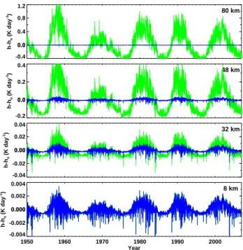
Figure 1 presents time series of the solar heating rate de-viation from the 1950–2006 mean values at different heights as calculated with the developed scheme. Calculations were done for an equatorial ozone profile and an overhead Sun as-suming 24 h illumination with the use of daily varying SSI provided on the SOLARIS website (2008). Changes in
so--0.4 0.0 0.4 0.8 1.2
0.0
h-h
o
(K day
-1)
80 km
-0.2 0.0 0.2 0.4
0.0
h-h
o
(K day
-1)
48 km
-0.04 -0.02 0.00 0.02 0.04
0.00
h-h
o
(K day
-1)
32 km
1950 1960 1970 1980 1990 2000
Year -0.004
-0.002 0.000 0.002 0.004
0.000
h-h
o
(K day
-1)
8 km
Fig. 1. Time series of the solar heating rate deviation from the
1950–2006 mean values in the troposphere (8 km), stratosphere (32 km), near the stratopause (48 km) and in the upper mesosphere (80 km). Blue: variability only in TSI is taken into account. Green: variability in SSI is taken into account. An overhead Sun and equa-torial ozone profile are considered in calculating the solar heating rates.
lar heating associated with changes in TSI (blue) and in SSI (green) are shown. As seen from Fig. 1, taking into account variability in TSI only provides a reasonable solar heating signal in the troposphere, where absorption in visible and near-infrared regions dominates the heating rates, but sig-nificantly underestimates it in the middle atmosphere. In this case the signal is very small (less than 0.0012 K day−1
from solar minimum to maximum at 8 km) and has a rela-tively weak variation with height. With variability in SSI in-cluded, the solar signal considerably increases with height as absorption at shorter wavelengths becomes more important. In this case, the shortwave heating rates between solar min-imum and maxmin-imum vary by about 0.03, 0.3 and 1 K day−1 at 32, 48 and 80 km levels, respectively.
2.2 EPP parameterization
In these simulations we limit our ionization sources to au-roral zone medium and high energy electrons, solar coro-nal mass ejection protons and galactic cosmic rays. Electron fluxes are measured by NOAA low earth orbit satellites, pro-ton fluxes are measured by the NOAA GOES geostationary satellites, and galactic cosmic ray intensity is measured by surface neutron monitors.
For all EPP types the NOxand HOxproduction rates were
determined from the energy deposition rate,E(eV g−1s−1), following the work of Porter et al. (1976). The ionization rate,I(cm−3s−1), is given by
I= ρ E
35.4 (1)
whereρis the air density in g cm−3and the ionization energy is 35.4 eV. The production of NOxis given by
PNOx=1.25I (2)
and 45 % ofPNOx is assumed to produce N(
4S)while 55 %
is assumed to go into N(2D). The latter is added to the pro-duction of NO and O since the reaction of N(2D)with O2
to form these products is rapid compared to the reaction of N(4S)with O2, which is very temperature dependent. The
production of HOxis given by
PHOx=a I (3)
wherea(z) is a height dependent function that varies from a value of 2 at 40 km to zero above 90 km and is an ap-proximation based on the typical variation found in Fig. 2 of Solomon et al. (1981). The actual production rate has a nearly linear dependence on the logarithm of the ioniza-tion rate with a negative slope depending on altitude. For example, around 75 km it falls from 1.93 to 1.3 as the ion-ization rate increases from 10 to 100 000 cm−3s−1. In the lower mesosphere and stratosphere the dependence of the production rate on the ionization rate is very small. So the ap-proximation has the greatest effect on auroral zone electron precipitation in our simulations. As shown in later sections, auroral zone HOxdoes not survive transport into the
strato-sphere due to its short photochemical lifetime so the impact on ozone and hence the dynamics of the middle atmosphere is not important.
It is assumed here thatPHOxcontributes equally to the
pro-duction of H and OH. Below 40 km,a(z)is taken to have a constant value of two. This assumption is a limitation since work with a detailed ion chemistry model (Verronen et al., 2006) indicates that HNO3 is an important direct product
through ion-ion recombination reactions with secondary OH production via photodissociation. As noted by Verronen et al. (2006) assuming a constant HOxproduction leads to an
un-derestimation of HOxduring sunrise and sunset which also
affects ozone loss, but only lasts for a short period outside polar regions.
Aurora Peak Ionization Rate (77 km)
1980 1985 1990 1995 2000 2005 1010-1
0
101
102
103
104
105
(ions cm
-3 s -1)
SPE Peak Ionization Rate (50 km)
1980 1985 1990 1995 2000 2005 10-1
100
101
102
103
104
(ions cm
-3 s -1)
GCR Peak Ionization Rate (12 km)
1980 1985 1990 1995 2000 2005 20
25 30 35 40 45 50
(ions cm
-3 s -1)
F10.7 Coronal Index
1980 1985 1990 1995 2000 2005 Year
0 50 100 150 200 250 300
Flux (10
22 W m -2 hz -1)
Fig. 2. Timeseries of peak ion pair production for aurora (top
panel), SPEs (second panel) and GCR (third panel). Auroral zone electrons and SPEs data is daily but GCR data is monthly. The F10.7 index variation is shown in the bottom panel.
Figure 2 shows the time series of the ion pair produc-tion rate for the three types of EPP used in the model along with the F10.7 solar variability index (adjusted Pentic-ton/Ottawa 2800 MHz solar flux, http://www.ngdc.noaa.gov/ stp/solar/flux.html). Auroral activity maximizes during the descending stage of the solar cycle. SPEs tend to cluster dur-ing solar maximum years when coronal activity is enhanced. GCR is anti-correlated with the solar cycle due to the com-plex heliospheric modulation driven by solar magnetic activ-ity.
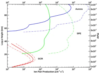
The vertical profiles of the peak ion pair production rate are shown in Fig. 3 based on the parameterizations described below. Auroral zone ionization maximizes in the upper mesosphere and above with a high energy tail that penetrates into the lower mesosphere. SPEs can have maximum ioniza-tion below the stratopause depending on the energy spectrum of the solar protons (Jackman et al., 2005). The GCR profiles peak around 13 km and there is about a factor of two differ-ence between solar maximum and minimum conditions.
2.2.1 Electron precipitation
measures the high energy electron fluxes. The MEPED data from 1979 through 2006 was used (NOAA/POES website, 2008). Data gaps were filled using the method of singular spectrum analysis (Kondrashov and Ghil, 2006).
The low energy MEPED channel (under 30 keV) was not used as electrons with this energy are deposited primarily above 100 km and the model lid. The thermospheric gen-eration of NOxvia extreme ultraviolet radiation, x-ray
radi-ation and ionizradi-ation by low energy EPP is not included in the model. This limitation manifests itself during solar max-imum periods when NOxincreases relative to solar minimum
conditions near the winter poles are several times smaller than observed. In observations (Hood and Soukharev, 2006) and model studies which include a more comprehensive ther-mosphere and low energy electron ionization (Marsh et al., 2007), there is a NOx variation of about 100 % during the
solar cycle as low as the stratopause.
However, the medium and high energy electrons consid-ered here are sufficient to produce mesospheric NOx
val-ues typical of solar minimum conditions (not shown). This reflects three constraints on the contribution of the region above the model lid to lower altitudes. Firstly, during descent in the lower thermosphere and upper mesosphere region air parcels experience large meridional excursions through wave action. In the polar region of both hemispheres between 80 and 100 km there are wintertime zonal wavenumber 2 planetary waves which propagate eastward (Sandford et al., 2008; Tunbridge and Mitchell, 2009). These waves have peak meridional winds of about 20 m s−1and have a two day period but occur for episodes lasting a week or more (Tun-bridge and Mitchell, 2009). There are also longer period os-cillations peaking above 80 km at high latitudes in the NH. They are eastward and westward traveling and have a zonal wavenumber 1 structure (Pancheva et al., 2008). The period of these waves is predominantly 16 and 23 days and their peak meridional wind amplitudes exceed 20 m s−1 during major SSW events but are not negligible at other times during winter. They are also very deep with vertical wavelengths in excess of 50 km. It is likely that the SH has analogous dis-turbances which reflect stratospheric vortex deformation, but with characteristics reflecting the large interhemispheric dif-ference in polar vortex behaviour. When taken together with the fact that the area of the polar night declines with altitude, these waves will contribute to significant loss of NOxthrough
long-distance transport into lower latitudes and photochemi-cal conversion back into N2.
Secondly, the descent of air between 100 and 80 km in the winter polar regions is frustrated by the fact that in both hemispheres the zonal wind undergoes a reversal in this layer (e.g., McLandress et al., 2006; Liu et al., 2010). Associated with this wind reversal is a layer where the meridional cir-culation changes sign and the flow is equatorward with lit-tle downward descent rather than poleward and downward. These results are model based but there is observational evi-dence to support them (e.g., Beagley et al., 2000). The large
Aurora
SPE
GCR 20
40 60 80
Log-p Height (km)
1x10³ 3x10² 1x10² 3x101 1x101 3x100 1x100 3x10⁻¹ 1x10⁻¹ 3x10⁻² 1x10⁻² 3x10⁻³ 1x10⁻³
(hPa)
100 101 102 103 104 105 Ion Pair Production (cm-3 s-1)
100 101 102 103 104 105
Fig. 3.Vertical pressure profiles of the time mean ion pair
produc-tion rate for auroral zone electrons (blue), SPEs (green), and GCR (red). The time average for SPEs is done only for the fraction of the time when ionization exceeds 100 pairs cm−3s−1at some altitude. The dash-dot curves represent maximum and minimum ionization for the 1979 through 2006 period. Minimum ionization is signifi-cant only for GCR.
wave diffusivity at these altitudes to some extent overcomes this large scale transport reversal and drives downgradient tracer fluxes. However, there is no simple transport conduit linking the low energy auroral region above 100 km with the mesosphere during winter.
The zonal wind reversals also result in a structure that supports barotropic and baroclinic instability and contributes to the growth of large amplitude Rossby wave disturbances (McLandress et al., 2006). As noted above, this reduces the survival of any thermospheric NOx during descent through
the MLT.
Thirdly, the density decreases exponentially with height. In the vicinity of the mesopause, between 80 and 90 km, the scale height is about 4 km, so the atmospheric density expe-riences about a 30-fold reduction between 80 and 100 km. A tracer originating above 100 km will experience a similar or greater reduction factor in mixing ratio during descent to 80 km depending on diffusion. Eddy and wave diffusion in-creases with height due to amplification of waves on account of density decrease. In the mesosphere the wave energy spec-trum has a−5/3 slope (e.g., Koshyk et al., 1999), which in-dicates a turbulent-like mixing regime. Observations of NOy
transport (e.g., Urban et al., 2009; Orsolini et al., 2009) indi-cate that there is attenuation of mixing ratios in descending plumes of air at the poles. Mixing ratio conservation would require a volumetric collapse of descending tracer plumes but instead they disperse.
values was used for subsequent calculations. This approach gives an average daily peak intensity that is biased on the high side. However, for the simulations presented here the peak NOx value of ∼5 ppmv in the polar regions between
80 and 90 km, agrees well with observations (Randall et al., 2009). A more sophisticated statistical model tying observed electron fluxes on orbit tracks to their spatial and temporal distribution in the auroral oval would be more accurate. The dependence of the flux on energy was approximated by a piece-wise exponential fit following Callis et al. (1998). The energy deposition was obtained using the range-energy ex-pression from Gledhill (1973) and the 80◦-isotropic energy distribution function from Rees (1989).
A parameterized auroral oval was used to obtain a 3-D distribution of electron energy deposition from the vertical profile calculated. The auroral oval is a modified version of the scheme from Holzworth and Meng (1975) based on the formulation of Feldstein (1963). The modification for the auroral horizontal distribution,H, was as follows:
H (φ,θ )=
exp(−((θg(φ,θ )−θc)/δθp)2),if θg> θc
exp(−((θg(φ,θ )−θc)/δθe)2),if θg≤θc (4)
θc =θe+0.3(θp−θe)
δθp=2(θp−θc)
δθe =(θc−θe)
(5)
whereθe andθp are the equatorial and polar corrected
ge-omagnetic latitude limits of the auroral oval, respectively, from the Holzworth and Meng (1975) scheme. This mod-ification was made to improve the realism of the auroral oval distribution when compared to the statistical model of the Space Weather Prediction Center of NOAA (see http: //www.swpc.noaa.gov/pmap/index.html). The map from ge-ographic longitude (φ) and latitude (θ) on the model grid to corrected geomagnetic latitude (θg(φ,θ )) was calculated
of-fline using an updated version of the GEOCGM program of Tsyganenko et al. (1987).
Hourly values of the auroral electrojet (AE) index (WDC website, 2008) were used to specify the size of the oval using the relation for theQindex from Starkov (1994). The orien-tation of the oval follows the Sun. The parameterized auroral oval resets Q values to six when they exceed this number, so that more NOxis deposited in the polar night than should be
during intense geomagnetic storms. In addition, the highest energy electrons are assumed to be distributed in the same auroral oval as the lower energy electrons when in fact rel-ativistic electrons are deposited in the sub-auroral belt (e.g., Brown, 1966). However, the relativistic electrons account for a small fraction of the NOxproduction and this limitation of
the scheme is not significant.
2.2.2 SPEs
For SPEs the daily energy deposition rate vertical profiles were obtained from the dataset of Jackman (2006). The hor-izontal distribution of the energy deposition was approxi-mated by axially symmetric caps centered on the geomag-netic poles with a diameter of about 60 degrees (Jackman et al., 2005). A smooth Gaussian squared transition was as-sumed starting with a value of one at 65◦and decreasing to zero at 45◦in geomagnetic coordinates with a 5◦scaling fac-tor to minimize Gibbs fringing since CMAM uses spectral transport.
2.2.3 GCR
Ionization effect of GCR was computed using the CRAC:CRII (Cosmic Ray induced Atmospheric Cascade: Application for Cosmic Ray Induced Ionization) model (Usoskin and Kovaltsov, 2006) extended toward the upper at-mosphere (Usoskin et al., 2010). The model is based on the full Monte-Carlo simulation of the cosmic ray induced atmo-spheric cascade and provides computations of the ionization rate in 3-D. The accuracy of the model is within 10 % in the troposphere and lower stratosphere, and up to a factor of two in the mesosphere (Bazilevskaya et al., 2008). The tempo-ral variability of the GCR energy spectrum, which is a result of the solar modulation in the heliosphere, is parameterized via the variable modulation potential, which is computed on a monthly basis using the data from the world network of ground-based neutron monitors (Usoskin et al., 2005). The final time-dependent ionization rate was computed using the following parameters: altitude (quantified via the barometric pressure), geomagnetic latitude (quantified via the geomag-netic cutoff rigidity computed in the framework of IGRF-10 model (IAGA/V-MOD website, 2008) and solar activity (quantified via the modulation potential).
3 Regression model
DJF Aurora-Reference
-90 -60 -30 00 30 60 90 0
20 40 60 80
Height (km)
DJF SPEs-Reference
-90 -60 -30 00 30 60 90 0
20 40 60 80
DJF GCR-Reference
-90 -60 -30 00 30 60 90 0
20 40 60 80
-7.00 -5.00 -3.00 -1.00 -0.50 -0.10 -0.05 0.00 0.05 0.10 0.50 1.00 4.00
-90 -60 -30 00 30 60 90 0
20 40 60 80
Height (km)
-90 -60 -30 00 30 60 90 0
20 40 60 80
-90 -60 -30 00 30 60 90 0
20 40 60 80
-3.00 -2.00 -1.00 -0.50 -0.10 -0.05 0.00 0.05 0.10 0.50 1.00 2.00 3.00
-90 -60 -30 00 30 60 90 Latitude (deg)
0 20 40 60 80
Height (km)
-90 -60 -30 00 30 60 90 Latitude (deg)
0 20 40 60 80
-90 -60 -30 00 30 60 90 Latitude (deg)
0 20 40 60 80
-4.00 -2.00 -1.00 -0.50 -0.10 -0.05 0.00 0.05 0.10 0.50 1.00 2.00 4.00
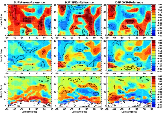
Fig. 4. Run mean, December–February mean differences compared to the reference run for auroral zone electrons (left), SPEs (center)
and GCR (right) showing zonal wind (top, m s−1), temperature (middle, K) and mass streamfunction (bottom, kg m−1s−1, values outside the (−4,4) interval not plotted). Solid and dashed contours denote regions with 95 % and 90 % confidence levels, respectively. These two contours are the same for all subsequent figures.
M(t )=a0+a1sin(π
t
2)+a2cos(π t 2)+ a3sin(π t )+a4cos(π t )+bt+
cSF10.7(t )+d1UQBO1(t )+d2UQBO2(t )+
eSAD(t )+fMEI(t )+gEESC(t )+ǫ(t ) (6) wheretis in seasons (three month means),SF10.7is the F10.7
index normalized by 100, andUQBO1andUQBO2are based
on the 30 hPa Singapore winds as in Randel and Wu (2007) and represent two orthogonal QBO wind components. The remaining fitting terms are the sulphate surface area density at 60 hPa, SAD (Hamill et al., 2006), the Multivariate ENSO index, MEI (Wolter and Timlin, 1998) and the EESC (New-man et al., 2007).
The height-latitude distributions of the F10.7 regression coefficient, c, are shown in Sect. 5. This coefficient repre-sents the fraction of the timeseries variation that projects onto the F10.7 timeseries. We chose the F10.7 index as a general representation of the solar cycle. The Ap index gives a better fit for the auroral component, as it reflects the variation of the solar wind streams. However, it does not serve the main purpose of this paper, which is to study all main EPP types including SPEs and GCR.
4 Impact of individual EPP types
The effect of the three EPP types on the long-term compo-sition and dynamics is presented in this section. These runs are single realizations from the 1979 through 2006 period spanned by the EPP data. This 28 yr period is too short to have a high confidence level for the dynamical response given dynamical variability. However, they do reveal the dis-tribution of the impact on composition and give some idea of the dynamical sensitivity.
4.1 Electron precipitation
DJF Aurora-Reference
-90 -60 -30 00 30 60 90 0
20 40 60 80
Height (km)
DJF SPEs-Reference
-90 -60 -30 00 30 60 90 0
20 40 60
80 DJF GCR-Reference
-90 -60 -30 00 30 60 90 0
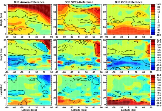
20 40 60 80
-100 -50 -30 -20 -10 -5 0 2 7 15 40 80 1900
-90 -60 -30 00 30 60 90 0
20 40 60 80
Height (km)
-90 -60 -30 00 30 60 90 0
20 40 60 80
-90 -60 -30 00 30 60 90 0
20 40 60 80
-75.0 -30.0 -15.0 -7.5 -1.5 -0.8 0.0 0.8 1.5 3.0 6.0 15.0 82.5
-90 -60 -30 00 30 60 90 Latitude (deg)
0 20 40 60 80
Height (km)
-90 -60 -30 00 30 60 90 Latitude (deg)
0 20 40 60 80
-90 -60 -30 00 30 60 90 Latitude (deg)
0 20 40 60 80
-60.0 -30.0 -10.0 -5.0 -2.0 -0.5 0.0 0.5 1.0 3.0 5.0 10.0 17.0
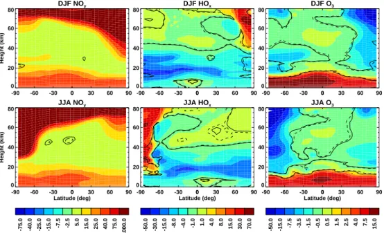
Fig. 5. Run mean, December–February mean NOy(top, %), HOx(middle, %) and O3(bottom, %) differences for auroral zone electrons,
SPEs and GCR runs compared to the reference run.
The change in the NH polar vortex shows a statistically significant increase of its diameter in the stratsophere be-low 30 km. The associated temperature shows a quadrupole structure with significance above 90 % only around 50◦ to 60◦N in the lower stratosphere, where it cools, and in the stratopause region where it warms. The Brewer-Dobson cir-culation change has three layers between 50◦and 80◦N with increased strength below 25 km, weakening between 25 and 40 km and an increase above only to 75◦N. However, the Brewer-Dobson circulation change is not statistically signif-icant. This highlights the limitations of using the Student-t test for the atmosphere, which has non-Gaussian statistics (e.g., Yoden et al., 2002). Presumably there is a unique meridional circulation change associated with the zonal wind change. However, this may not be the case and the lack of statistical confidence could reflect a degeneracy in the dy-namical response.
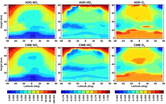
The DJF mean, run mean NOy, HOxand ozone differences
for the run with auroral zone ionization and the reference run are shown in Fig. 5 (left panels). There is a large increase of NOyin the winter auroral production zone down to about
30 km. We note that above 40 km the NOyis essentially NOx.
In the summer auroral production zone the increase extends only down to 65 km. The difference in the polar regions be-tween the summer and winter is, of course, that the exposure of NOxto sunlight in the polar summer results in its
destruc-tion, viz.,
NO+hν→N+O (R1)
N+NO→N2+O (R2)
which is modulated by reaction with O2and OH,
N+O2→NO+O (R3)
N+OH→NO+H (R4)
There is also a significant increase of NOx at all latitudes
above 70 km. In the SH summer at middle and polar latitudes and between the surface and 20 km, NOyincreases by over
5 % and this feature is most likely a remnant of downward transport of NOy during the previous winter. At these
alti-tudes the photochemical lifetime of NOyis long. Also, polar
vortex interior air is “fossilized” in the summertime due to weak mixing (Orsolini , 2001; Orsolini et al., 2003). In the Northern Hemisphere during winter, below 40 km, there is a modest decrease of NOyin this latitude range (but not
statis-tically significant) which may be associated with a strength-ening of the Brewer-Dobson circulation. Since the disturbed state of the winter NH stratosphere prevents significant trans-port of NOyinto this region from above, an increase in
trans-port of low NOyair from the tropics could lead to this
reduc-tion.
The left central panel for HOxshows an increase in both
the summer and winter polar mesosphere due to the EPP HOx
source from water vapour. The largest percentage increase occurs in the winter polar regions partly due to the reduced background HOxin winter. Above 70 km at low and middle
latitudes there is no comparable increase of HOx as
by photolysis of water vapour. Also, to a lesser extent, the difference is because the photochemical lifetime of HOxis
shorter (under a day in contrast to 5 days for NOx).
In the summer hemisphere, below 40 km there is a de-crease in HOx. This may be due to changes in the sources
and/or sinks of HOx. As can be seen in the lowest left panel,
ozone has also decreased and so one of the sources of HOx,
viz. reaction of O(1D)(produced from photolysis of ozone) with H2O, CH4 and H2 would decrease. There is also a
source from the photolysis of HNO3, which has increased
in this region (top left panel, NOyis primarily HNO3at these
altitudes). With respect to changes in sinks, the sink via the reaction OH+HNO3→H2O+NO3has increased as well.
The lowest left panel shows that the largest effect on ozone is in the winter polar region above 50 km. This reflects that auroral zone electron ionization occurs in the upper meso-sphere polar regions and the HOxproduced (see middle left
panel) leads to reduction of ozone via
H+O3→OH+O2 (R5)
OH+O→H+O2 (R6)
Net:O+O3→2O2 (R7)
and
O+HO2→OH+O2 (R8)
O+OH→H+O2 (R9)
H+O2+M→HO2+M (R10)
Net:O+O→O2 (R11)
This effect can also be seen in the summer polar region above 60 km. There is ozone loss of between 2 and 5 % be-tween 25 and 40 km in both the winter and summer hemi-spheres. The additional ozone loss is driven by increases in NOxthat survived from the previous winter via
O+NO2→NO+O2 (R12)
NO+O3→NO2+O2 (R13)
Net:O+O3→2O2 (R14)
There is a transition from O3 destruction to production
in the lowermost stratosphere and troposphere (Brasseur and Solomon, 2005). Above roughly 20 km the NOx loss cycle
(Reactions R12–R14) dominates while below the O3 smog
production reactions become important, e.g.
NO+HO2→NO2+OH (R15)
CO+OH+O2→CO2+HO2 (R16)
NO2+hν+O2→NO+O3 (R17)
Net:CO+2O2+hν→CO2+O3 (R18)
Thus, the increase in NOxbelow 20 km leads to an increase
of ozone. The decrease in the HOxis more than compensated
by the increase in NOx.
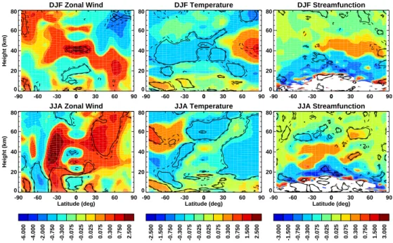
The SH winter, June through August (JJA), dynamical dif-ference compared to the redif-ference run is shown in Fig. 6 (left
panels). There is a small but statistically significant reduction in the strength of the SH polar vortex (Fig. 6, top left panel) as measured by the reduction in the zonal wind and also by the increase in temperature below 60 km (Fig. 6, middle left panel). The mass streamfunction shows a statistically sig-nificant increase poleward of 60◦S below 40 km, which is consistent with the increased temperature and weaker zonal wind above 20 km. Consideration of Eliassen-Palm flux di-vergence (not shown) shows that increased wave drag, i.e. more negative Eliassen-Palm flux divergence, is responsible for the dynamical changes rather than direct radiative effects from chemical constituent changes. Note that in the SH neg-ative anomalies in the mass streamfunction indicate intensi-fication in contrast to the NH where this applies to positive anomalies due to the change in sign of the Coriolis parame-ter at the equator. It is also notable that the Brewer-Dobson circulation change in the SH is hemispheric in scale, as in the NH, in spite of the fact that the ionization impact on compo-sition occurs at high latitudes (see Figs. 5 and 7). The tropo-spheric response is opposite in sign compared to the NH and statistically significant.
There is an equatorward shift in the extratropical jet with a weakening in middle latitudes and intensification around 30◦S. A possible explanation for this feature can be inferred from the work of Polvani and Kushner (2002). They demon-strated using a mechanistic model that as the stratospheric polar vortex weakens, the subtropical jet moves equatorward. There was no threshold behaviour in the response, so it is plausible that their results apply to the weak changes seen here.
Figure 7 (left panels) shows the atmospheric chemical dif-ference for the SH winter, JJA. The response reflects differ-ences in transport between the two hemisphere. For example, the penetration of extra NOxin the SH polar winter is more
contained within the vortex than for DJF in the NH. In ad-dition, the increase and penetration in the SH winter extends to 30 km for an 80 % change compared to 45 km in the NH winter. The SH summer NOxis higher than for NH summer,
which reflects the higher amounts in SH at the end of winter compared to the NH.
The NH polar vortex tends to be weaker and more dis-turbed compared to the SH vortex due to hemispheric dif-ferences in planetary wave forcing (Andrews et al., 1987). So perturbations associated with composition changes, un-less they are large, are not likely to alter the NH state signifi-cantly. As noted above, the more disturbed NH vortex results in increased destruction of auroral zone NOxby exposure to
sunlight during descent as air parcels are transported out of the polar night by planetary wave induced mixing and vortex deformation. So the chemical impact on dynamics is more limited in the NH compared to the SH.
As expected, there is an increase in HOxin the SH winter
polar region above 50 km as a result of EPP and the small background HOxin the reference run. There is also a small
JJA Aurora-Reference
-90 -60 -30 00 30 60 90 0 20 40 60 80 Height (km) JJA SPEs-Reference
-90 -60 -30 00 30 60 90 0 20 40 60 80 JJA GCR-Reference
-90 -60 -30 00 30 60 90 0 20 40 60 80 -7.00 -5.00 -3.00 -1.00 -0.50 -0.10 -0.05 0.00 0.05 0.10 0.50 1.00 4.00
-90 -60 -30 00 30 60 90 0 20 40 60 80 Height (km)
-90 -60 -30 00 30 60 90 0
20 40 60 80
-90 -60 -30 00 30 60 90 0 20 40 60 80 -3.00 -2.00 -1.00 -0.50 -0.10 -0.05 0.00 0.05 0.10 0.50 1.00 2.00 3.00
-90 -60 -30 00 30 60 90 Latitude (deg) 0 20 40 60 80 Height (km)
-90 -60 -30 00 30 60 90 Latitude (deg) 0 20 40 60 80
-90 -60 -30 00 30 60 90 Latitude (deg) 0 20 40 60 80 -4.00 -2.00 -1.00 -0.50 -0.10 -0.05 0.00 0.05 0.10 0.50 1.00 2.00 4.00
Fig. 6. Run mean, June–August mean differences compared to the reference run for auroral zone electrons (left), SPEs (center) and GCR
(right) showing zonal wind (top, m s−1), temperature (middle, K) and mass streamfunction (bottom, kg m−1s−1, values outside the (−4,4) interval not plotted).
JJA Aurora-Reference
-90 -60 -30 00 30 60 90
0 20 40 60 80 Height (km) JJA SPEs-Reference
-90 -60 -30 00 30 60 90
0 20 40 60 80 JJA GCR-Reference
-90 -60 -30 00 30 60 90
0 20 40 60 80 -100 -50 -30 -20 -10 -5 0 2 7 15 40 80 1900
-90 -60 -30 00 30 60 90
0 20 40 60 80 Height (km)
-90 -60 -30 00 30 60 90
0 20 40 60 80
-90 -60 -30 00 30 60 90
0 20 40 60 80 -75.0 -30.0 -15.0 -7.5 -1.5 -0.8 0.0 0.8 1.5 3.0 6.0 15.0 69.0
-90 -60 -30 00 30 60 90
Latitude (deg) 0 20 40 60 80 Height (km)
-90 -60 -30 00 30 60 90
Latitude (deg) 0 20 40 60 80
-90 -60 -30 00 30 60 90
Latitude (deg) 0 20 40 60 80 -80.0 -30.0 -10.0 -5.0 -1.0 -0.5 0.0 0.5 1.0 3.0 5.0 10.0 15.0
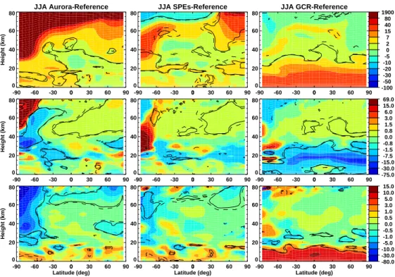
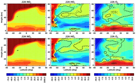
Fig. 7.Run mean, June–August mean compared to the reference run for auroral zone electrons (left), SPEs (center) and GCR (right) showing
winter (Fig. 5, left panels), there is a 5 % decrease in HOxin
mid-latitudes between 50 and 70 km and 30◦to 75◦N (Fig. 5, middle left panel). Another region of decrease in the NH winter occurs between 30 and 40 km. For the SH winter, the decrease has strengthened and also has become more exten-sive in the stratosphere extending below 20 km (Fig. 7, mid-dle left panel). Above 60 km, HOxis produced by photolysis
of H2O. Below 60 km it is largely through reaction of O(1D)
with H2O, CH4and H2. This would suggest that O(1D)has
decreased in the high latitude stratosphere and lower meso-sphere, and to some extent this is reflected by the reduction of ozone in polar regions in SH winter. Whereas there is a substantial decrease in HOxin the SH winter between 10
and 40 km, there is a much smaller decrease of HOxin this
altitude range in the NH winter polar regions. The loss of HOxin the winter polar region in the stratosphere is due to
reaction with the additional NOxtransported from the upper
mesosphere.
The ozone decrease in both the NH and SH polar vortex (Figs. 5 and 7, lower left panels) is caused in the upper re-gions by HOxincreases while in the lower regions it is due
to increased NOxsince HOxdoes not survive transport from
the mesosphere into the stratosphere. Below 20 km at all lat-itudes of the SH in JJA there are regions of enhanced ozone with peak significance values above 90 % but less than 95 %. These increases in ozone are compatible with the increase of NOxproduced by auroral zone electrons of which a fraction
is transported to the atmospheric layer below 20 km and the smog reactions noted above. In addition, there is increased transport of O3 into the lowermost stratosphere and
tropo-sphere by the enhanced Brewer-Dobson circulation in the SH (Fig. 6, bottom left panel). It should be noted that these fig-ures are showing percentage differences which can be large due to the typically low ozone values in the troposphere. So even if the ozone anomaly near the pole above 15 km is nega-tive due to chemical loss, it can be posinega-tive in the troposphere due to increased transport.
4.2 SPEs
The DJF change in the polar vortex shows an increase in diameter in the stratosphere as in the case of auroral zone electrons (Fig. 4, top middle panel). However, the change is only statistically significant below 25 km. There is also a cooling in the lower stratosphere between 30◦and 70◦N. The Brewer-Dobson circulation response has a three layer structure similar to that with the auroral zone case, except the middle layer corresponding to reduced strength is more intense and is statistically significant between 30 and 40 km poleward of 60◦N. In contrast to the auroral zone response, there is a statistically significant poleward shift of the tropo-spheric jet structure, with weakening in the subtropics and intensification in middle latitudes. Unlike in the SH winter for auroral zone electrons and SPEs (see below), this tro-pospheric zonal wind change does not appear to follow the pattern identified by Polvani and Kushner (2002). However,
the structure of the stratospheric polar vortex change is more complex and less statistically significant. So it is not im-mediately apparent which regions are key to mediating the stratosphere-troposphere coupling.
Figure 5 (middle panels) shows the differences in NOy,
HOx and ozone for SPEs in DJF. The SPEs NOx response
pattern is similar to, but much weaker, than that of the auro-ral zone case for the mesosphere. Even though there is more ionization produced by individual SPEs in the upper strato-sphere and lower mesostrato-sphere during each event, it is sporadic and averages out to similar or lower values over the duration of the simulation. In addition, the SPEs NOxis formed lower
in the atmosphere and so a given amount created will appear with a lower mixing ratio near the stratopause as compared to the mesopause. The low values of NOxabove 70 km in the
NH are due to both downward transport from the lower ther-mosphere where the model lid boundary condition is 1 ppmv, and the fact that SPEs ionization peaks around 60 km so there is much less ionization above 70 km compared to the auroral zone case. The higher values of NOx above 70 km in the
summer hemisphere (here the NH) are due to the meridional circulation pattern. There is upwelling in the summer polar regions, which lofts the NOxin the mesosphere with
trans-port above the mesopause. An NOyincrease between 2 and
7 % is present in the SH from the surface to 40 km. There is some accumulation above the extratropical tropopause as with the auroral zone case. Between 15 and 25 km in the SH polar region the response is negative but with no statis-tical confidence. This suggests a high level of variability in this region for this season which is likely due to dynamical processes. There is evanescent penetration of Rossby waves above the summertime zero zonal wind line that can extend as high as 25 km in addition to significant generation of oro-graphic gravity waves by the extreme Antarctic topography (Andrews et al., 1987).
The SPEs HOx response shows an increase in the polar
lower mesosphere and upper stratosphere since it is being produced in this region in contrast to the auroral zone case, where it is produced above 60 km and does not survive trans-port into the stratosphere. Below 40 km there is a decrease in HOxthrough reaction of OH with HNO3, which has been
augmented. There is also a reduction in ozone, the source of O(1D)(and thus HOx), in this region. There is a large
nega-tive correlation between the distribution of the NOyand HOx
anomalies between 20 and 40 km in high latitudes.
the previous winter and reflects a summertime contribution from SPEs. In the troposphere, there is an increase of ozone which could be due to increased NOxbut the effects of an
in-creased Brewer-Dobson circulation could also be important. However, the changes are not statistically significant.
From the difference plots in Fig. 6 (middle panels) it can be seen that the JJA SH polar vortex is weakened in high latitudes and also becomes broader judging by the larger in-crease in the zonal wind equatorward of 60◦S. The peak neg-ative zonal wind anomaly is comparable to the auroral zone case. However, the temperature change is weaker and not statistically significant near the pole but is statistically sig-nificant in middle latitudes between 20 and 40 km. There is also a warming in the tropics not present in the auroral zone case in this layer. It is also not statistically significant. This middle latitude cooling and tropical warming reflects the weakening of the residual circulation in middle and low latitudes in this layer of the stratosphere (Fig. 6, lower middle panel). The Brewer-Dobson circulation shows an intensifica-tion similar to the auroral zone case in high latitudes below 40 km with some statistical significance below 30 km. There is also a statistically significant weakening of the circulation between 55 and 65 km. This dynamical pattern is the classi-cal response to a loclassi-calized wave drag change consisting of a quadrupole temperature anomaly accompanied by a vertical dipolar mass streamfunction anomaly (Haynes et al., 1991). In the troposphere there is a zonal circulation anomaly that resembles the auroral zone case and is opposite in sign to DJF.
For JJA NOyand HOxchanges (Fig. 7, middle panels) the
response is almost the mirror of DJF changes (Fig. 5, mid-dle panels). For JJA, the ozone impact is not as pronounced as for the auroral zone case and is only statistically signifi-cant between 20 and 30 km (see lower middle and lower left panels of Fig. 7). This reflects the fact that the SPEs are spo-radic. It also suggests that the containment properties of the stronger SH polar vortex for NOxproduced by SPEs are less
important. The NOxproduction of SPEs occurs in the lower
mesosphere and upper stratosphere and is at lower altitudes compared to the auroral zone case, so that NOxdoes not have
to survive transport from the upper mesosphere. The JJA vor-tex response (Fig. 6, top middle panel) suggests that ozone perturbations of a few percent in the polar region between 20 and 30 km can both induce a weakening of the strength and an increase of the diameter of the SH polar vortex above 25 km.
Vortex variability does play a role in the SPEs case as can be seen by the absence of a significant ozone loss in the NH summer: any NOx produced during the previous
win-ter at higher altitudes experiences greawin-ter loss compared to the SH. Between the tropopause and 25 km during DJF in the SH there is an ozone increase of 3 to 10 % which is sta-tistically significant at the 80 % confidence level (contours not shown). At these heights this increase is likely due to the smog reactions on account of the NOxincrease (about 5 %),
which more than balances the HOxdecrease. This
summer-time ozone increase is smaller in scale in the NH.
4.3 GCR
The DJF change in the dynamics induced by GCR is different compared to auroral zone electrons and SPEs (Fig. 4, right panels). There is some increase of the polar vortex diameter below 30 km but it is not statistically significant. There is no warming near the pole below this altitude as in the other two cases, albeit non-significant. The structure of the Brewer-Dobson circulation change is quite different, with a general weakening in the NH stratosphere. Between 30◦and 70◦N in the lowermost stratosphere and upper troposphere there is a statistically significant temperature change that resem-bles the SPEs case and which is associated with a poleward shift of the tropospheric jet in the same region. As with the other two EPP types, the stratospheric effect is obscured by NH vortex variability. Yet there is a coherent response in the troposphere. Assuming the Student-t test is good enough to identify any coherent structure in the stratosphere, if one ex-isted, this suggests that different stratospheric states produce similar tropospheric dynamical changes.
For the stable SH polar vortex regime the impact of GCR is pronounced as opposed to the NH winter. The dynami-cal response in JJA shows some similarities to the other two EPP types (Fig. 6, right panels). The polar vortex weakens to a similar degree between 60◦S and 80◦S above 30 km and this feature is statistically significant. But the reduction is not associated with a vortex diameter increase and there is a weakening in middle and low latitudes as well. The temper-ature change in the SH reaches lower latitudes and it appears that the wave drag change is broader meridionally compared to the auroral zone and SPEs cases. The GCR temperature change is most similar to that produced by auroral zone elec-trons, but with a large region of statistically significant cool-ing in the tropics and subtropics of the stratosphere. The residual circulation intensification in the SH extends over the depth of the stratosphere with a 95 % confidence region be-tween the tropopause and 40 km poleward of 60◦S. GCR is producing a change of the same sign in wave drag over a broader latitude span in spite of being a weaker source of ionization than the other two types of EPP. As shown below, the GCR effect on ozone is not confined to the polar regions or low altitudes. In the troposphere, there is a statistically significant change in the zonal jet structure that is similar to the auroral zone and SPEs cases and is of opposite sign to the DJF response in the NH hemisphere. It appears to be due to weakening of the stratospheric polar vortex, as with the other two EPP types.