Lubomir Kostal*, Petr Lansky, Ondrej Pokora
Department of Computational Neuroscience, Institute of Physiology, Academy of Sciences of the Czech Republic, Prague, Czech Republic
Abstract
During the stationary part of neuronal spiking response, the stimulus can be encoded in the firing rate, but also in the statistical structure of the interspike intervals. We propose and discuss two information-based measures of statistical dispersion of the interspike interval distribution, the entropy-based dispersion and Fisher information-based dispersion. The measures are compared with the frequently used concept of standard deviation. It is shown, that standard deviation is not well suited to quantify some aspects of dispersion that are often expected intuitively, such as the degree of randomness. The proposed dispersion measures are not entirely independent, although each describes the interspike intervals from a different point of view. The new methods are applied to common models of neuronal firing and to both simulated and experimental data.
Citation:Kostal L, Lansky P, Pokora O (2011) Variability Measures of Positive Random Variables. PLoS ONE 6(7): e21998. doi:10.1371/journal.pone.0021998
Editor:Zheng Su, Genentech Inc., United States of America
ReceivedApril 26, 2011;AcceptedJune 9, 2011;PublishedJuly 22, 2011
Copyright:ß2011 Kostal et al. This is an open-access article distributed under the terms of the Creative Commons Attribution License, which permits unrestricted use, distribution, and reproduction in any medium, provided the original author and source are credited.
Funding:This work was supported by AV0Z50110509, Centre for Neuroscience LC554, and the Grant Agency of the Czech Republic project P103/11/0282. The funders had no role in study design, data collection and analysis, decision to publish, or preparation of the manuscript.
Competing Interests:The authors have declared that no competing interests exist.
* E-mail: [email protected]
Introduction
One of the most fundamental problems in computational biology is the problem of neuronal coding, the question of how information is represented in neuronal signals [1,2]. The discharge activity of neurons is composed of series of events called action potentials (or spikes). It is widely accepted, that information in neuronal systems is transferred by employing these spikes. The shapes and durations of individual spikes are very similar, therefore it is generally assumed that the form of the action potential is not important in information transmission. When a stimulus is presented, the responding neuron usually produces a transient response followed by a sustained one, which is often treated as stationary in time [3] . The firing rate of the sustained part of the response depends on the stimulus, however, the stimulus can be also ‘‘encoded’’ in the statistical structure of the interspike intervals (ISI) by thetemporal coding[1,4–6].
While the description of neuronal activity from the rate coding point of view is relatively straightforward [7] , the temporal code allows infinite number of alternatives. Spike trains with equal firing rates may turn out to be different under various measures of their statistical structure beyond the firing rate. For example, even more than a half century ago, coefficient of variation (cv) of ISIs was reported to encode information about light intensity in adapted cells of the horseshoe crab [1,8]. Similarly, changes in the level of bursting activity, also characterized bycv, are reported to be the proper code for edge detection in certain units of visual cortex [9]. In general, the bursting nature of neuronal firing is commonly described bycv [10].
In order to describe and analyze the way information is represented in spike trains, methods for their mutual comparison are needed. Although the ISI probability density function (or histogram of data) usually provides a complete information, one needs quantitative methods [11–13], especially since a visual inspection of the density shape can be misleading. Here we restrict
our attention to the measures of the neuronal firing precision, e.g., of the the ISI distribution dispersion. We investigate the properties of the standard deviation, the entropy-based dispersion and the Fisher information-based dispersion. Although standard deviation is used ubiquitously and is almost synonymous to the ‘‘measure of statistical dispersion’’, we show, that it is not well suited to quantify some aspects of spiking activity that are often expected intuitively [4,14]. We will show, that the diversity or randomness of ISIs is better described by entropy-based or Fisher information-based dispersions. The difference between entropy and Fisher informa-tion descripinforma-tions lies in the fact that the Fisher informainforma-tion describes how ‘‘smooth’’ is the distribution, while the entropy describes how ‘‘even’’ it is. The ‘‘smoothness’’ and ‘‘evenness’’ might be at first thought interchangeable, but we show that it is not the case.
The illustration of the proposed methods is provided on simple and frequently employed models of stationary neuronal activity, given by lognormal, gamma and inverse Gaussian distributions of ISIs. Finally, we apply the theory on experimental data obtained by recording the spontaneous activity of rat olfactory neurons [15].
Methods
Statistical methods and methods of probability theory and stochastic point processes are widely applied to describe and to analyze neuronal firing [16–18]. The probabilistic description of spiking times results from the fact, that the positions of spikes cannot be predicted exactly, only the probability that the spike occurs is given [18]. Thus, under suitable conditions, the ISI or time-to-first spike after the stimulus onset can be described by a continuous positive random variable. We denote this random variable asT. Complete description ofTis given by its probability density functionf(t), defined on½0,?).
different dispersion measures described in the literature and employed in different contexts, e.g., standard deviation, inter-quartile range [19], mean difference [20] or the coefficient of local variance [13]. The measures have the same physical units asT.
Standard deviation
By far, the most common measure of dispersion is the standard deviation, s, defined as the square root of the second central moment of the distribution. The correspondingrelativedispersion measure is known as the coefficient of variation,cv,
cv~
s
Eð ÞT , ð1Þ
where Eð ÞT is the mean value of T. Exponential distribution implies cv~1, however, this values of cv may occur for other distributions as well.
Entropy based dispersion
The randomness of a probability distribution can be defined as the measure of ‘‘choice’’ of possible outcomes. Bigger choice results, intuitively, in greater randomness. For discrete probability distributions such measure of randomness is provided by the Shannon entropy, which is known to be a unique, consistent with certain natural requirements [21]. The Shannon entropy is generally infinite for continuous variables, and therefore it cannot be used for our purposes. Formally, the notion ofdifferential entropy,
h(f), of probability density functionf(t), is introduced as
h(f)~{ ð
T
f(t) lnf(t)dt, ð2Þ
however, the valueh(f)can be positive or negative and cannot be by itself used as a measure of randomness [22].
In order to obtain a properly behaving quantity, the entropy-based dispersion,sh, was proposed in [23],
sh~exp½h(f){1: ð3Þ
The interpretation of sh relies on the asymptotic equipartition property theorem and the entropy power concept [22]. Namely, since for the exponential probability density function
fexp(t)~1=Eð ÞT exp½{t=Eð ÞT holds h(fexp)~1zEð ÞT we see, thatshis the standard deviation of such exponential distribution, which satisfiesh(fexp)~h(f). Informally, the value ofsh is bigger for those random variables, which generate more diverse (or unpredictable) realizations.
Analogously to Eq. (1), we define the relative entropy-based dispersion coefficient,ch, as
ch~
sh
Eð ÞT : ð4Þ
Note, that Eq. (4) can be equivalently written as
ch~exp{DKL½f(t)Efexp(t)
, ð5Þ
whereEð ÞT is the mean value ofTand
DKL½f(t)Efexp(t)~ ð
T
f(t) ln f(t)
fexp(t)
dt ð6Þ
is the Kullback-Leibler distance of the probability density f(t) from the exponential density with the same mean asf(t). From Eq. (5) follows thatchis essentially (up to the scale) equivalent to the measure of spiking randomness, g, proposed in [4], since
ch~eg{1.
From the properties of the Kullback-Leibler distance in Eq. (5) follows, that the maximum value ofch isch~1, which occurs if and only iff(t)is exponential [22].
Fisher information based dispersion
The Fisher information is a measure of the minimum error in estimating a parameter of a distribution. In a special case of the location parameter, the Fisher informationJ(f)does not depend on the parameter itself, and can be expressed directly as a functional of the densityf(t)([22], p.671),
J(f)~ ð ?
0
Llnf(t)
Lt
2
f(t)dt: ð7Þ
We illustrate that the value ofJ(f) is small for smoothly-shaped probability densities. Any locally steep slope or the presence of modes in the shape of f(t) increases J(f) [24]. Due to the derivative in Eq. (7), certain regularity conditions are required on
f(t). In this paper we consider only the densities for whichJ(f) takes finite values. Further theoretical considerations are however beyond the scope of this paper.
The units ofJ(f)correspond to the inverse of the squared units of T, therefore we propose the Fisher information-based dispersion measure,sJ, as
sJ~ 1 ffiffiffiffiffiffiffiffiffi J(f)
p : ð8Þ
In analogy with Eqns. (1) and (4) we define the relative dispersion coefficientcJ as
cJ~
sJ
Eð ÞT : ð9Þ
For exponential distribution holdscJ~1, however, this value is not specific only for the casef(t)~fexp(t).
Just aschis related to the Kullback-Leibler distance by Eq. (5), we note thatJ(f)can be written as [25]
J(f)~L 2D
KL½f(t{D)Ef(t)
LD2
D~0
: ð10Þ
Although Eq. (10) is not suitable for evaluation ofJ(f), it shows, that bothchandcJare connected on the fundamental level by the concept of the Kullback-Leibler distance.
Basic properties of the proposed measures
Standard deviation (or cv) measures essentially how off-centered, with respect to Eð ÞT , is the probability density of T
and it is sensitive to outlying values. On the other hand,cv does not quantify how random, or unpredictable, are the outcomes of
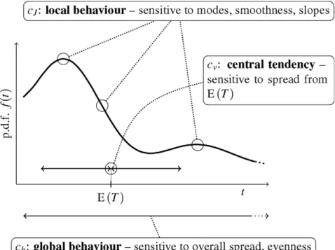
the dependence on the derivative of the probability density in Eq. (7)). Since multimodal densities can be more evenly spread than unimodal ones, the behavior ofch cannot be generally deduced fromcJ (and vice versa). The key features of the three considered dispersion measures are illustrated in Fig. 1.
A cartoon with typical density shapes resulting from a combination of cv, ch and cJ values range is shown in Fig. 2. Very small value of cv inevitably results in a density shapes concentrated aroundEð ÞT , and correspondingly small values ofch andcJ. The intermediate,cv^1, and upper range ofcvoffer more variable density shapes, wherecvandchare not sufficient for their classification and cJ can be employed for further description.
Note, that the number of possible scenarios is large and therefore Fig. 2 is not exhaustive.
Results
Common distributions of interspike intervals
We choose three widely employed statistical models of ISIs: gamma, inverse Gaussian and lognormal distributions, and analyze them by means of the three described dispersion coefficientscv,chandcJ.
Gamma distribution is one of the most frequent statistical descriptors of ISIs employed in analysis of experimental data Figure 1. Illustration of the main features of the studied measures.Schematic example of a probability density functionf(t)is shown. Although the evenness of the density (described bych) and its smoothness (described bycJ) are related, the sensitivity ofcJto modes and slopes enables it to differentiate shapes with otherwise equalcvandch.
doi:10.1371/journal.pone.0021998.g001
Figure 2. Illustration of a classification tree of probability densities based on typical values of the dispersion measures.Note, that not all combinations of values ofcv,ch,cJcan appear. Selected identification signs or examples of corresponding distributions, which are typical but not necessarily comprehensive, are written bellow the corresponding illustrative plots of densities.
[15,26,27]. Its probability density function parametrized by shape parameterkand scale parameterhis
f(t)~t
k{1expf{t=hg
C(k)hk , ð11Þ
whereC(z)is the gamma function [28]. The mean value of the distribution isEð ÞT ~khand the coefficient of variation is equal to
cv~1=
ffiffiffi k p
: ð12Þ
Forcv~1, i.e.k~1, the gamma distribution becomes exponential distribution. By parametrizing the density (11) by cv and substituting it into Eqns. (4) and (9) we obtain the entropy-based and Fisher information-based dispersion coefficients as functions ofcv,
ch~c2vC(c
{2 v ) exp
1z(c2 v{1)Y(c
{2 v ) c2 v {1
, ð13Þ
cJ~cv
ffiffiffiffiffiffiffiffiffiffiffiffiffiffi 1{2c2 v
q
for 0vcvv 1ffiffiffi 2
p , ð14Þ
whereY(z)~d
dzlnC(z)is the digamma function [28]. For details of the calculation of ch and cJ see Supporting Information S1. Note, that the gamma density is not differentiable at t~0 for
cv§1=pffiffiffi2, thuscJ is evaluated only for0vcvv1=pffiffiffi2.
The inverse Gaussian distribution is often used to describe neural activity and fitted to experimentally observed ISIs [26,29,30]. This distribution describes the spiking activity of a stochastic variant of the perfect integrate-and-fire neuronal model [18,31]. The probability density function of the inverse Gaussian distribution parametrized by its mean, m~Eð ÞT , and scale parametersis
f(t)~ ffiffiffiffiffiffiffiffiffiffiffiffiffiffi1 2ps2t3
p exp {(t{m) 2
2s2m2t
( )
: ð15Þ
The coefficient of variation is equal to
cv~
ffiffiffiffiffiffiffiffi ms2 p
ð16Þ
and the other dispersion coefficients can be expressed as (see Supporting Information S1)
ch~
ffiffiffiffiffiffi 2p e r
cvexp {
3 exp(c{2
v )K(1,0) {12,c
{2 v ffiffiffiffiffiffi 2p p cv
, ð17Þ
cJ~
ffiffiffi 2 p
cv
ffiffiffiffiffiffiffiffiffiffiffiffiffiffiffiffiffiffiffiffiffiffiffiffiffiffiffiffiffiffiffiffiffiffiffiffiffiffiffiffiffi 2z9c2
vz21c4vz21c6v
p , ð18Þ
whereK(1,0)(n,z)is the derivative of the modified Bessel function of the second kind,K(1,0)(n,z)~L
LnK(n,z)[28].
The lognormal distribution of ISIs, with some exceptions [32], is rarely presented as a result of a neuronal model. However, it represents a common descriptor in experimental data analysis [26,30]. The lognormal probability density function parametrized
by the mean,m, and standard deviation,s, of variablelnT is
f(t)~ ffiffiffiffiffiffiffiffiffiffi1 2ps2 p
texp
{(lnt{m) 2
2s2
( )
: ð19Þ
In this parametrization, the mean of the lognormal distribution is Eð ÞT ~expmzs2=2and the coefficient of variation is equal to
cv~
ffiffiffiffiffiffiffiffiffiffiffiffiffiffiffiffiffiffiffiffiffiffiffi expð Þs2 {1 q
: ð20Þ
The two other dispersion coefficients, expressed as functions ofcv, are (see Supporting Information S1)
ch~
ffiffiffiffiffiffi 2p e
r ffiffiffiffiffiffiffiffiffiffiffiffiffiffiffiffiffiffiffi ln(1zc2
v) 1zc2
v
s
, ð21Þ
cJ~
ffiffiffiffiffiffiffiffiffiffiffiffiffiffiffiffiffiffiffiffiffiffiffiffiffiffiffiffiffiffiffiffiffiffiffiffiffiffiffiffiffiffiffiffi ln(1zc2
v)
½1zc2 v
3
½1zln(1zc2 v)
s
: ð22Þ
The dependence ofchoncvis shown in Fig. 3, the dependence of cJ on cv is shown in Fig. 4, for all the three mentioned distributions. Obviously, the dependencies are not linear (even not monotonous) and thus neither ch nor cJ is equivalent to cv. Maxima ofchandcJoccur for differentcvvalues, confirming that each of the proposed dispersion coefficients provides a different point of view. We see, that bothchandcJas functions ofcvshow a ‘‘\’’ shape with maxima around cv¼: 1 (for ch) and around
cv¼: 0:5(forcJ). There is a reason why the maxima ofchandcJ tend to occur at these values ofcv. It can be shown by the methods of variational calculus, that there exists a unique distribution maximizingch: the exponential distribution for whichcv~1. Since some densities tend to resemble the exponential density if theircv is close to1, their maxima ofchoccur near thiscvvalue. Similarly, there exists a unique density maximizingcJ; it is given in terms of the Airy functions with cv~0:44. Analogously, densities with
cv&0:5 may resemble this distribution and thus attain the maximum ofcJ there. However, there exist distributions which does not attain the maximum ofcharoundcv~1or the maximum ofcJaroundcv~0:5. Detailed mathematical treatment of thech -and cJ-maximizing distributions is beyond the scope of the manuscript and will be published elsewhere.
Note, that the plots ofcJagainstcvappear like a scaled version of the plots ofchagainstcv, with the relative positions of the curves for each distribution preserved (to certain extent). In particular, whilechof the lognormal is always greater thanchof the inverse Gaussian, the ordering is reversed for thecJ forcvw2:2.
The dependence ofcJ onchis plotted in Fig. 5. We observe, thatch and cJ indeed do not describe the same qualities of the distribution, since a unique ch value does not correspond to a unique cJ value (and vice versa). Except for the gamma distribution, the dependence betweench and cJ forms a closed loop, wherech~cJ~0for bothcv?0andcv??.
Additionally, just asch andcJ are related tocv in Eqns. (13), (14), (17), (18), (21) and (22),chandcJcan also be related to higher statistical moments. For example, the skewnesscof the distribution is defined as the ratio of the third central moment and the third power of standard deviation. For gamma distribution holds
c~c3
vz3cv. Thus the curves depicted in Fig. 3 and Fig. 4 would retain their unimodal shapes if plotted in dependence onc.
Different distributions with equalcvand differentch(orcJ) can be found, and vice versa; see Fig. 3 (or Fig. 4) for examples. Therefore, it cannot be said in general that ch, cJ are more informative thancv. To provide an example in whichcJprovides a different view over cv and ch, we consider the folded normal
probability density with parametersa,bw0
f(t)~ ffiffiffiffiffiffiffiffi
2
b2p s
1zerf affiffiffi 2 p
b
{1
exp {(t{a) 2
2b2
" #
: ð23Þ
The shapes of the folded normal probability density function, Eq. (23), and gamma probability density function, Eq. (11), are compared in Fig. 6 forcv~0:69. Although their values ofchare very similar, the values ofcJ are very different. The reason lies mainly in the initial steep rise of the gamma density from zero.
Simulated data
To illustrate the accuracy of the estimators ccbhh and ccbJJ of dispersion coefficients ch and cJ, we simulated spike trains with gamma, inverse Gaussian and lognormal distributions of ISIs by employing the R and STAR software packages [26,33]. In all the simulations the mean ISI was fixed to1, while the coefficient of variation,cv, varied from0:05to4:00 in steps of0:05. In other words, we generated random samples from the mentioned distributions with given parameters. The spike trains represented by sample point processes were constructed by using the generated values as the time intervals (ISIs) between successive events (spikes). Five thousand spike trains, each consisting of 100 ISIs, were simulated for each of the values ofcv and for each of the three distributions.
In the first study, the parameters of the distributions were estimated by the maximum likelihood method. For the gamma distribution (11) the maximum likelihood estimators bkk and bhh
were found numerically (by minimizing the loglikelihood function). For the inverse Gaussian distribution (15) the maximum likelihood estimators were computed as
b m m~1
n Xn
i~1
ti, ð24Þ
Figure 3. Entropy-based dispersion coefficient, ch, in depen-dence on the coefficient of variation,cv.Three interspike interval models: gamma, inverse Gaussian and lognormal distribution, are employed. Bothcvandchdescribe ‘‘spread’’ of the interspike intervals, but from different points of view. Coefficient of variation,cv, quantifies how off-centered is the mass of the probability density function, whereas ch indicates how evenly is the mass distributed over all possible values. For all the shown distributions holdsch~0ascv?0or
cv??.
doi:10.1371/journal.pone.0021998.g003
Figure 4. Fisher information-based dispersion coefficient,cJ, as a function of the coefficient of variation, cv, for the same distributions as in Fig. 3.The coefficientcJgrows as the average of squared derivative of the probability density function (see Eq. (7)) becomes smaller, that means as the distribution of the interspike intervals becomes more smooth. This confirms that ‘‘smoothness’’ and ‘‘evenness’’ of the distribution (compare with Fig. 3) are different notions, although there are qualitative similarities:cJ~0forcv?0for all shown distributions, and cJ~0 as cv?? for both lognormal and inverse Gaussian distributions. Note, that dispersion coefficientcJ for the gamma distribution can be calculated only forcvv1=pffiffiffi2¼: 0:707. doi:10.1371/journal.pone.0021998.g004
Figure 5. The dispersion coefficientsch andcJ for the same distributions as in Figs. 3 and 4.The plot of dependencies between the two dispersion coefficients form closed curve for both inverse Gaussian and lognormal distribution. Starting from the origin and moving clockwise, the points on the loop correspond to the values ofcv growing from0to infinity. For gamma distribution,cJ is a common unimodal function ofch.
b s2
s2~1
n Xn
i~1 1
ti {1
b m
m: ð25Þ
Similarly, for the lognormal distribution (19) of ISIs, maximum likelihood estimators of the parameters are
b m m~1
n Xn
i~1
lnti, ð26Þ
b s2
s2~1
n Xn
i~1 lnti{bmm
ð Þ2: ð27Þ
The values of coefficient of variation, cv, were calculated by substitution of the maximum likelihood estimates into Eqns. (12), (16) or (20). Consequently, the other two dispersion coefficients,ccbhh and ccbJJ, were computed by substitution of the estimated cv into Eqns. (13) and (14) for the gamma distribution, into Eqns. (17) and (18) for the inverse Gaussian and into Eqns. (21) and (22) for the lognormal distribution.
In the second study, the coefficient of variation was estimated by commonly used moment method as the ratio of the sample standard deviation,bss, and the sample mean,T,
b cv
cv~b
s s
T, ð28Þ
for all the mentioned distributions. Both the entropy-based and Fisher information-based dispersion coefficients were then calcu-lated by substitution of estimate (28) into the same equations forccbhh andccbJJas with maximum likelihood estimates, in accordance to the respective ISI distribution.
The accuracy of the estimatesccbhhandccbJJwas studied for both the types of estimators. The results are depicted in Fig. 7 for the
maximum likelihood estimates, and in Fig. 8 for the moment estimates. In both figures two measures of the accuracy of the estimatorsccbhhandccbJJare plotted against the true values ofcv(those used for simulation). The first is the bias of the estimate,b(ch), defined as
b(ch)~ 1
n Xn
i~1
(ccchh,,ii{ch), ð29Þ
wheren~5000is the number of simulated spike trains andccchh,,iiis the value estimated from thei-th spike train. Analogous equation is used for evaluation ofb(cJ). The latter measure is the relative standard error, e(ch), expressed as the ratio of the standard deviation and the mean value of the estimate,
e(ch)~ 1
b(ch)zch
ffiffiffiffiffiffiffiffiffiffiffiffiffiffiffiffiffiffiffiffiffiffiffiffiffiffiffiffiffiffiffiffiffiffiffiffiffiffiffiffiffiffiffiffiffiffiffiffiffiffiffiffiffiffiffiffi 1
n{1 Xn
i~1 c ch,i
ch,i{½b(ch)zch
f g2
s
, ð30Þ
and analogously fore(cJ). This characteristics says how accurate the values of the estimator are when calculated from random sample of givencv. The relative standard deviation with respect to the mean value is dimensionless and therefore it is suitable for comparisons of the quality of different estimators ofchandcJ.
We observe qualitative similarities in the dependencies of both the bias and the relative standard error of the estimatorsccbhhandccbJJ. In general, we see that the estimators are biased (see panelsa,bin Figs. 7 and 8), but the values of bias of the moment estimators are approximately 10 times greater than the bias of the maximum likelihood estimators. For small values of cv the dispersion coefficients are underestimated and the bias becomes positive as
cvgrows. For gamma distribution, the bias ofccbhhstarts to decrease to zero after it attains its maxima forcv¼: 2, thusccbhhseems to be asymptotically unbiased estimator. On contrary, bias of ccbhh for inverse Gaussian and lognormal distribution grows ascv grows. There is also a difference between the maximum likelihood and moment estimatorccbhh: in the maximum likelihood case the bias of
b ch
ch for inverse Gaussian distribution is greater than for the lognormal, the difference seems to be negligible in the case of the moment estimator.
The bias ofccbJJlooks similar to the bias ofccbhhfor smallcv. But, in contrary to ccbhh, the bias ofccbhh starts to decrease slowly for large values of the coefficient of variation (cvw2). This fact can bee seen for both the inverse Gaussian and lognormal distribution. In the maximum likelihood case the bias ofccbJJis almost the same for both these distributions. The bias ofccbJJis greater for the lognormal than for inverse Gaussian distribution.
Focusing on the accuracy of the estimators (see panelsc, din Figs. 7 and 8), the shapes of the relative standard deviations ofccbhh andccbJJ are very similar, regardless of the ISI distribution and the method used for estimation. The relative standard deviations ofccbJJ look like scaled versions of analogous characteristics of ccbhh. For
cv?0they starts at a value less than0:1.
Ascv grows from zero, the relative standard deviation of the estimators decrease and attains its minima at aroundcv¼: 1:2(for
b ch
ch) andcv¼: 0:5(forccbJJ), respectively. It should be noted that these minima of relative standard deviations ofccbhhandccbJJ coincide with the maxima ofch andcJ (compare with Figs. 3 and 4). In other words, the estimates ccbhh and ccbJJ are most accurate for cv values where ch and cJ attain their theoretical maxima; but they are slightly negatively biased. For larger values of cv the relative standard deviations ofccbhhandccbJJare increasing functions ofcv. In addition, the values of relative standard deviations of the Figure 6. Comparison of probability density functions with
estimators for large cv values are ordered according to the ISI distribution. The order of the estimator accuracy (from high to low) is lognormal, inverse Gaussian and gamma distribution in the case of ccbhh, and inverse Gaussian, lognormal and gamma distribution in the case ofccbJJ.
Experimental data
In order to examine variability or irregularity of the ISIs in real neurons using the proposed dispersion coefficients, we apply the
measures on experimental data. The data come from extracellular recordings of olfactory receptor neurons of freely breathing and tracheotomizedrats. Spontaneous, single-unit action potentials were recorded. The single unit nature of the recorded spikes was controlled. The experimental procedures and data analysis were published in [15], where complete details are given. The groups are not distinguishable on the basis of firing frequency only. For our purpose only samples with sufficient number of observations were chosen. Analyzed dataset consists of 6 records of ISIs from Figure 7. Dispersion coefficients estimation by using the maximum likelihood method from simulated data.Bias (panelsa,b) and relative standard deviations (panelsc,d) of the dispersion coefficients estimatesccbhh(panelsa,c) andccbJJ(panelsb,d), in dependence on the true value of the coefficient of variation,cv, are shown. The depicted characteristics were estimated from simulated random samples drawn from inverse Gaussian (circles), lognormal (crosses) and gamma distribution (triangles). CoefficientccbJJfor gamma distribution (panelsb,d) can be computed for
cvv0:707only.
freely breathing rats and 11 records from tracheotomized rats. The sample sizes range from150to1500and all records were tested against nonstationarity.
All samples were fitted with inverse Gaussian distribution (15) as a commonly used distribution of ISI. The histogram of ISIs of typical record and fitted probability density function are depicted in Fig. 9. The mean,m, and the scale parameterswere estimated by maximum likelihood method. The fit of the data to the inverse Gaussian distribution was checked by Kolmogorov-Smirnov test. The null hypothesis was not rejected on the 5% level in any sample. The dispersion coefficientscv, chandcJ were calculated
by substitution of the estimated parameters into Eqns. (16), (17) and (18).
The values of estimated dispersion coefficients are summarized and shown as box-and-whisker plots in Fig. 10. Generally, the two categories, tracheotomized and freely breathing, do not differ signifi-cantly in the medians ofcv,chorcJ. Although the ranges of the values overlap in both categories, the values of the criteria seem to be relatively specific with respect to thefreely breathingcategory. The difference between mean values are greater than between medians. However, we can observe that thetracheotomizedcategory achieves higher values ofcv and lower values of bothch and cv
Figure 8. Dispersion coefficients estimation by using the moment method.The structure of the panels and the notation are equivalent to those in Fig. 7, except that the estimatesccbvv, and consequentlyccbhhandccbJJ were estimated by the moment method.
than the freely breathing category. Taking into account the interquartile-range and the range between the whiskers, the Fisher information-based dispersion coefficient,cJ, seems to be the best of the three examined coefficients to distinguish the two categories for this data. Both groups of rats were compared by employing one-sided variant of the Mann-Whitney test to the three respective dispersion coefficients. However, due to the small sample sizes, no differences between the two groups were confirmed at 95% confidence level.
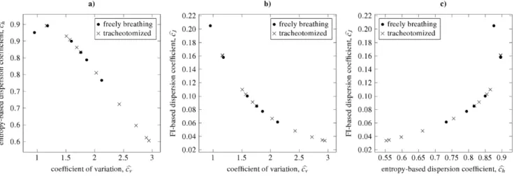
Moreover, obtained scatterplots of pairs of the dispersion coefficientschandcJare shown in Fig. 11. The two categories of rats are best distinguishable in panel c), for the tracheotomized category having lower values ofchtogether with lower values ofcJ than the latter one. Note also the positions of the points in panelc), which confirm that there can be two different cJ values corresponding to uniquechvalue.
Discussion
In recent years, information-based measures of signal regularity or randomness have gained significant popularity in various
branches of science [24,34–37]. In this paper, we constructed dispersion-like quantities based on these information measures and applied them to the description of neuronal ISI distributions. In particular, we continued the effort initiated in [4,23] by taking into account a variant of Fisher information, which has been employed also in different contexts [24,38–41].
We are motivated by the difference between frequently mixed up notions of ISI variability and randomness, which, however, represent two different concepts. Consider, for example, a spike train consisting of ‘‘long’’ and ‘‘short’’ ISIs with no serial correlations. By adding ‘‘medium’’ length ISIs we do not increase the spiking variability, contrary to what expected intuitively, but decrease it. On the other hand, since the count of ISI of different lengths increases, the spiking randomness is increased. Further-more, even if conventional analysis of two spike trains reveals no difference, the spike trains may still differ in their randomness and the difference is tractable with relatively limited amount of data [4].
Additionally, by considering the Fisher information-based dispersion coefficient,cJ, we show that ISI randomness (increasing with diversity of the ISI lengths) and probability density ‘‘smoothness’’ are related, but still different notions. For example, all of the tested distributions are ‘‘maximally smooth’’ forcv¼: 0:5 and ‘‘maximally even’’ (maximum ISI randomness) forcv¼: 1.
The statistical properties of the parametric estimations ofcvand ofchandcJ consequently, are illustrated on simulated data. The results show that the accuracy of the dispersion coefficients depends on the distribution. However, similar property can be found: estimated values ofchas well as ofcJbecome accurate at the point of maxima of these dispersion coefficients, regardless on the used ISI distribution. It is shown that the ISI distribution as well as the method used for estimation of the parameters from the sample highly influence the bias of the estimatorsccbhhandccbJJ.
In this paper, we used the parametrical estimates ofcv,ch,cJfor both simulated and experimental data analyses. Specific paramet-ric family of distributions was assumed and only the parametres were estimated. On the other hand, it is natural to ask for the non-parametric versions of the estimators. The non-non-parametric estimate ofcv is simply calculated by using the first two sample moments. Recently [42], discussed disadvantages of this estimator, Figure 9. Histogram of interspike intervals from a typical
record of the data.The thick curve shows the shape of probability density function fitted by the maximum likelihood method. Estimated dispersion coefficients arecv¼: 1:59,ch¼: 0:85andcJ¼: 0:10. doi:10.1371/journal.pone.0021998.g009
Figure 10. Box-and-whisker plots of estimated dispersion coefficients.The coefficientscv(panela),ch(panelb), andcJ(panelc) estimated from the experimental data (spontaneously active rat olfactory neurons) are shown for two categories: freely breathing and tracheotomized rats. The lower and upper sides of the boxes denotes the first (Q1) and third (Q3) quartile, thick lines inside the boxes are medians, triangles denote mean
values. The whiskers show the lowest and greatest data value betweenQ1{1:5|IQRandQ3z1:5|IQR(whereIQR~Q3{Q1is interquartile range).
stressing out its bias. Non-parametric estimates of the entropy are known [43,44], and we found ch can be estimated reliably. As regards the non-parametric estimate of cJ, approaches based either on spline interpolation of the empirical cumulative distribution function [45] or on specialized kernel-based method for the estimation of the probability density function [46] can be used. Nevertheless, the estimation of the Fisher information-based dispersion coefficient cJ is a complex task. Preliminary results of our work in progress are promising.
The coefficients were also evaluated from the experimental data, spontaneous action potentials of olfactory receptor neurons in tracheotomized and freely breathing rats. Assuming the inverse Gaussian model, the three estimated dispersion coefficients quantify small differences in the two categories. Taking into account their variability, cJ seems to be the best measure for distinguishing the categories. Other approach use the pairs of
coefficientscv,chandcJ to discriminate between the groups. For the analyzed data, the pair of values ch and cJ seems to be the most effective choice.
Supporting Information
Supporting Information S1 Detailed calculation of the coefficients ch and cJ for the gamma, inverse Gaussian and lognormal distributions.
(PDF)
Author Contributions
Conceived and designed the experiments: LK PL OP. Analyzed the data: LK OP. Contributed reagents/materials/analysis tools: LK PL OP. Wrote the paper: LK OP.
References
1. Perkel DH, Bullock TH (1968) Neural coding. Neurosci Res Prog Sum 3: 405–527.
2. Stein R, Gossen E, Jones K (2005) Neuronal variability: noise or part of the signal? Nat Rev Neurosci 6: 389–397.
3. Johnson DH, Glantz RM (2004) When does interval coding occur? Neurocomputing 59: 13–18.
4. Kostal L, Lansky P, Rospars JP (2007) Review: Neuronal coding and spiking randomness. Eur J Neurosci 26: 2693–2701.
5. Nemenman I, Lewen GD, Bialek W, de Ruyter van Steveninck RR (2008) Neural coding of natural stimuli: Information at sub-millisecond resolution. PLoS Comput Biol 4: e1000025.
6. Theunissen F, Miller JP (1995) Temporal encoding in nervous systems: A rigorous definition. J Comput Neurosci 2: 149–162.
7. Lansky P, Rodriguez R, Sacerdote L (2004) Mean instantaneous firing frequency is always higher than the firing rate. Neural Comput 16: 477–489.
8. Ratliff F, Hartline HK, Lange D (1968) Variability of interspike intervals in optic nerve fibers of limulus: Effect of light and dark adaptation. Proc Natl Acad Sci USA 60: 464–469.
9. Burns BD, Pritchard R (1964) Contrast discrimination by neurons in the cat’s visual cerebral cortex. J Physiol 175: 445–463.
10. Fenton AA, Lansky P, Olypher AV (2002) Properties of the extra-positional signal in hippocampal place cell discharge derived from the overdispersion in location-specific firing. Neuroscience 111: 553–566.
11. Buracas GT, Albright TD (1999) Gauging sensory representations in the brain. Trends Neurosci 22: 303–309.
12. Victor JD, Purpura KP (1997) Metric-space analysis of spike trains: theory, algorithms and application. Network: Comput Neural Syst 8: 127–164. 13. Shinomoto S, Kim H, Shimokawa T, Matsuno N, Funahashi S, et al. (2009)
Relating neuronal firing patterns to functional differentiation of cerebral cortex. PLoS Comput Biol 5: e1000433.
14. Kostal L, Lansky P, Zucca C (2007) Randomness and variability of the neuronal activity described by the Ornstein-Uhlenbeck model. Network: Comput Neural Syst 18: 63–75.
15. Duchamp-Viret P, Kostal L, Chaput M, Lansky P, Rospars JP (2005) Patterns of spontaneous activity in single rat olfactory receptor neurons are different in normally breathing and tracheotomized animals. J Neurobiol 65: 97–114. 16. Kass RE, Ventura V, Brown EN (2005) Statistical issues in the analysis of
neuronal data. J Neurophysiol 94: 8–25.
17. Moore GP, Perkel DH, Segundo JP (1966) Statistical analysis and functional interpretation of neuronal spike data. Annu Rev Physiol 28: 493–522. 18. Tuckwell HC (1988) Introduction to Theoretical Neurobiology, Volume 2. New
York: Cambridge University Press.
19. Kendall M, Stuart A, Ord JK (1977) The advanced theory of statistics. Vol. 1: Distribution theory. London: Charles Griffin.
20. Chakravarty SR (1990) Ethical social index numbers. New York: Springer-Verlag.
21. Ash RB (1965) Information Theory. New York: Dover.
22. Cover TM, Thomas JA (1991) Elements of Information Theory. New York: John Wiley and Sons, Inc.
23. Kostal L, Marsalek P (2010) Neuronal jitter: can we measure the spike timing dispersion differently? Chin J Physiol 53: 454–464.
24. Frieden BR (1998) Physics from Fisher information: a unification. New York: Cambridge University Press.
25. Kullback S (1968) Information theory and statistics. New York: Dover. 26. Pouzat C, Chaffiol A (2009) Automatic Spike Train Analysis and Report
Generation. An Implementation with R, R2HTML and STAR. J Neurosci Methods 181: 119–144.
27. Reeke GN, Coop AD (2004) Estimating the temporal interval entropy of neuronal discharge. Neural Comput 16: 941–970.
Figure 11. Dependencies between different dispersion coefficients for the same experimental data as in Fig. 10.The data was fitted by inverse Gaussian distribution and from maximum likelihood estimators of its parameters the dispersion coefficients were computed. Two categories of data are distinguished: tracheotomized and freely breathing rats. There are small differences in the two categories, as quantified by all the three coefficients. See Figs. 3, 4 and 5 for inverse Gaussian distribution to see the complete curves of the dependencies.
28. Abramowitz M, Stegun IA (1965) Handbook of Mathematical Functions, With Formulas, Graphs, and Mathematical Tables. New York: Dover.
29. Berger D, Pribram K, Wild H, Bridges C (1990) An analysis of neural spike-train distributions: determinants of the response of visual cortex neurons to changes in orientation and spatial frequency. Exp Brain Res 80: 129–134.
30. Levine MW (1991) The distribution of the intervals between neural impulses in the maintained discharges of retinal ganglion cells. Biol Cybern 65: 459–467. 31. Lansky P, Sato S (1999) The stochastic diffusion models of nerve membrane
depolarization and interspike interval generation. J Peripher Nerv Syst 4: 27–42. 32. Bershadskii A, Dremencov E, Fukayama D, Yadid G (2001) Probabilistic properties of neuron spiking time-series obtained in vivo. Eur Phys J B 24: 409–413.
33. R Development Core Team (2009) R: A language and environment for statistical computing. Vienna, Austria: R Foundation for Statistical Computing. 34. Bercher JF, Vignat C (2009) On minimum Fisher information distributions with
restricted support and fixed variance. Inform Sciences 179: 3832–3842. 35. Berger AL, Della Pietra VJ, Della Pietra SA (1996) A maximum entropy
approach to natural language processing. Comput Linguist 22: 39–71. 36. Della Pietra SA, Della Pietra VJ, Lafferty J (1997) Inducing features of random
fields. IEEE Trans on Pattern Anal and Machine Int 19: 380–393.
37. Di Crescenzo A, Longobardi M (2002) Entropy-based measure of uncertainty in past lifetime distributions. J Appl Probab 39: 434–440.
38. Frieden BR (1990) Fisher information, disorder, and the equilibrium distributions of physics. Phys Rev A 41: 4265–4276.
39. Telesca L, Lapenna V, Lovallo M (2005) Fisher information measure of geoelectrical signals. Physica A 351: 637–644.
40. Vignat C, Bercher JF (2003) Analysis of signals in the Fisher–Shannon information plane. Phys Lett A 312: 27–33.
41. Zivojnovic V (1993) A robust accuracy improvement method for blind identification usinghigher order statistics. In: IEEE Internat. Conf. Acous. Speech. Signal Proc., 1993. ICASSP-93. volume 4. pp 516–519.
42. Ditlevsen S, Lansky P (2011) Firing variability is higher than deduced from the empirical coefficient of variation. Neural Comput;in press.
43. Vasicek O (1976) A test for normality based on sample entropy. J Roy Stat Soc B 38: 54–59.
44. Tsybakov AB, van der Meulen EC (1994) Root-n consistent estimators of entropy for densities with unbounded support. Scand J Statist 23: 75–83. 45. Huber PJ (1974) Fisher information and spline interpolation. Ann Stat 2:
1029–1033.