ISSN 1549-3644
© 2005 Science Publications
Corresponding Author: R.J. Bhansali, Division of Statistics and Probability, Department of Mathematical Sciences University of Liverpool, Peach Street, Liverpool, L69 7ZL,
Inverse Correlations for Multiple Time Series and Gaussian Random Fields
and Measures of Their Linear Determinism
1
R.J. Bhansali and
2L. Ippoliti
1
Division of Statistics and Probability, Department of Mathematical Sciences
University of Liverpool, L69 7ZL, Liverpool
2
Department of Quantitative Methods and Economic Theory
University ‘G. d’Annunzio’, Viale Pindaro 42, 65127 Pescara, Italy
Abstract: For a discrete-time vector linear stationary process, {X(t)}, admitting forward and backward autoregressive representations, the variance matrix of an optimal linear interpolator of X(t), based on a knowledge of {X(t-j), j≠0}, is known to be given by Ri(0)-1 where Ri(0) denotes the inverse variance of the process. Let A=Is−Ri(0)1R(0)1, where R(0) denotes the variance matrix of {X(t)} and I an s s×s, identity matrix. A measure of linear interpolability of the process, called an index of linear determinism, may be constructed from the determinant, Det[Is−A], of Is−A=Ri(0)−1R(0)−1. An alternative measure is constructed by relating tr[Ri(0)−1], the trace of Ri(0)-1, to tr[R(0)]. The relationship between the matrix A and the corresponding matrix, P, obtained by considering only an optimal one-step linear predictor of X(t) from a knowledge of its infinite past, {X(t-j),j>0}, is also discussed. The possible role the inverse correlation function may have for model specification of a vector ARMA model is explored. Close parallels between the problem of interpolation for a stationary univariate two-dimensional Gaussian random field and time series are examined and an index of linear determinism for the latter class of processes is also defined. An application of this index for model specification and diagnostic testing of a Gaussian Markov Random Field is investigated together with the question of its estimation from observed data. Results are illustrated by a simulation study.
Key words: Spatial series analysis, time series analysis, gaussian random fields, gaussian markov random fields, inverse correlation function, linear predictor
INTRODUCTION
Consider a vector-valued linear stationary process, {X(t)}, (t∈N), where N =[0, ±1,...] denotes the set of all integers. Suppose that {X(t)} satisfies the following assumption:
Assumption 1: For each t∈N, X(t)=
[
X1(t), X2(t),…,Xs(t)
]
′ admits the following one-sided moving averagerepresentation:
( )
( ) (
) ( )
0
, B 0 s j
X t ∞ B j ε t j I
=
=
∑
− = , (1)where ε(t)=
[
ε1(t),ε2(t),...,εs(t)]
' and {ε(t)} is a purely random process:( )
0,( ) (
)
' u BEε t = Eε t ε t u− =δ V (2)
for all t, u∈N, VB is nonsingular, δu=1, u=0, δu=0, u≠0,
the B(j) are (s×s) matrices satisfying
0
( ) ,
j B j
∞
=
< ∞
∑
0
( ) j 0, | | 1,
j
Det ∞ B j z z
=
≠ ≤
∑
and
1 1
s s
uv
u v
C C
= =
=
∑∑
denotes the sum of the absolute values of an (s×s) matrix C=[Cuv], ( ,u v=1, 2,..., ;s s≥1), Det
[ ]
C the determinant of C, C' its transpose, I an (ss ×s) identity matrix and 0 a matrix or vector of zeroes.For all t, v∈N, the matrix covariance and correlation functions of
{ }
X(t) are defined by{
}
( ) ( ) ( ) ' ,
R v =E X t X t v− r(v)=R(0)−1R(v),
respectively and the matrix spectral density function by
( ) ( )
1(
)
2 ( ) exp( ),
-v
f µ π − ∞ R v ivµ π µ π
=−∞
=
∑
− ≤ ≤Assumption 1 ensures that
{ }
X(t) admits a backward autoregressive representation:0
( ) ( ) ( ), (0) s j
A j X t j ε t A I
∞
= − = =
∑
(3)and a forward autoregressive representation[1]:
0
( ) ( ) ( ), (0)
F F F s
j
A j X t j ε t A I
∞
=
+ = =
where εF(t)=
[
ε1F(t),ε2F(t),...,εsF(t)]
' and {εF(t)} is purely random with( )
0,( ) (
)
'F F F u F
Eε t = Eε t ε t u− =δ V , VF is nonsingular and
1
0 0
( ) j ( ) j ,
j j
A j z B j z
− ∞ ∞ = = =
∑
∑
0 ( ) j A j ∞= < ∞
∑
, . 1 , 0 ) j ( 0 j ≤ ≠ ∑
∞ = z z ADet F j
We may, accordingly, write[2]
( ) ( ) ( ) 1 0 j F F 1 0 j F 1 1 0 j B 1 0 j 1 ) ij exp( )' j ( A V ) ij exp( ) j ( A 2 ) ij exp( )' j ( A V ) ij exp( ) j ( A 2 f − ∞ = − ∞ = − − ∞ = − ∞ = − µ − µ π = µ µ − π = µ
∑
∑
∑
∑
and f(µ) is nonsingular.
The inverse, [ ( )]f µ −1, of f(µ) has all the essentials
properties of a spectral density function[4] and the inverse spectral density function of
{
X t( )}
may be defined by . )] ( f [ ) 2 ( ) (fiµ = π −2 µ −1 Let
( )
∫
ππ −
µ µ µ
= fi( )exp(iv )d v
Ri , (v=0, ±1,...)
define the inverse covariance function of {X(t)} and ) v ( Ri ) 0 ( Ri ) v (
ri = −1 the inverse correlation function, where Ri(v)'=Ri(-v). It follows that[3], fi(µ) admits a
Fourier expansion:
1
( ) (2 ) ( ) exp( ).
v
fi µ π − ∞ Ri v ivµ
=−∞
=
∑
−For a univariate process, s=1, the role of inverse correlation function for time series model identification is examined by several authors; see Cleveland[4], Chatfield[5], McClave[6], Bhansali[7-9], among others. A
somewhat different application of this function, namely for estimating the interpolation error variance and a related R2 measure, is suggested by Battaglia and Bhansali[10].
In this paper, the potential role the inverse correlation function may have for model specification of a multivariate time series as well as that of a Gaussian Markov random field, GMRF, is examined. Following Battaglia[13], an inverse process, {Yi(t)}, of
{X(t)} is defined by relating this process to the error process, ζ(t), of the linear interpolator, and several related measures of linear interpolability, called measures linear determinism, for multivariate time series are defined. An application of the inverse correlation function for specifying a vector autoregressive moving average model is also considered. The results here show that because of the ’arrow of time’ and the associated notions of ’past’ and
’future’, the role of this function for model identification of a multivariate time series is somewhat limited and possibly confined to special classes of models. However, by contrast, we show that the inverse correlations define the parameters of a GMRF and hence play a fundamental role in specifying its structure. Based on this observation, an R measure of 2 linear interpolability of Gaussian Random Fields is introduced and potential applications of this index for model assessment and criticism are discussed. The inverse correlations of a GMRF also define the correlation structure of the residuals of a model specified for a GMRF. We discuss therefore how this property may be applied for diagnostic testing of a fitted GMRF model. The question of how to estimate the index of linear determinism for a Gaussian random field is also considered and two different estimates of the index are defined, namely, a nonparametric estimate based on a ’window’ estimate of the spectral density function of the field, and a parametric likelihood estimate. We finally provide some simulation results. Inverse process and the linear interpolator: Let
{
X t( )}
satisfy Assumption 1 and suppose that X(t) is unknown for a fixed t. The question of how to construct an optimal linear estimate of X(t) from a knowledge of {X(t-j),j≠0} is known as the problem of linear interpolation[11]. Examples of situations where aquestion of this type arises include the problem of outlier detection and estimation of missing values for a multivariate time series, analysis of spatial data collected over a narrow but long rectangular lattice[12]
and spatio-temporal processes.
Properties of the inverse process: As is well known[11], for each t,
0
ˆ ( ) ( ) ( )
u
X t ri u X t u
≠
= −
∑
− (5)provides an optimal linear interpolator of X(t), where the ri(u) denote the inverse correlation function of
{
X t( )}
. Moreover, if ˆ ( )t X t( ) X t( )ζ = −
denotes the error of the optimum linear interpolator, the interpolation error variance matrix is given by
{ }
{
}
1ˆ ˆ
var ( ) { ( ) ( )}{ ( ) ( )}' (0)
t E X t X t X t X t
Ri ζ − = − − = Now, let
( ) (0) ( ) ( ) ( )
u
Yi t Ri ζ t ∞ Ri u X t u
=−∞
= =
∑
−We have
{
( )}
0,{
( ) ( ) '}
( ) t,u 0, 1,... ;(
)
E Yi t = E Yi t Yi t u− =Ri u = ±
same as the inverse covariance function of
{ }
X(t) and vice versa. As in Battaglia[13]{
Yi(t)}
may be called the Inverse Process of{ }
X(t) .Now, see Masani[14],
{
Yi(t)}
admits forward andbackward linear representations:
0
( ) ( ) ' ( ),
j
Yi t ∞ A j τi t j
=
=
∑
+ (6)0
( ) F( ) ' F( ),
j
Yi t ∞ A j τi t j
=
=
∑
−where τi(t)=VB−1ε(t), i (t) V (t), F 1 F
F = ε
τ − and {τi(t)}
and {τiF(t)} define the inverse processes of
{ }
ε(t) and )},t (
{εF respectively. We have,
{ }
i(t) 0, E{
i (t)}
0,Eτ = τF =
{
i(t) i(t u)'}
( )
V Eτ τ − =δu B -1{
i (t) i (t u)'}
( )
V(
t,u 0, 1,...)
EτF τF − =δu F -1 = ±
Measures of linear determinism: It follows from (5) that E{ζ(t)X(t-v)'}=0, for all v≠0 and hence that E{ζ(t) Xˆ (t)'}=0. Thus, the individual components of ζ(t) and Xˆ (t) are mutually uncorrelated and we may write,
var{X(t)}=var{ Xˆ (t)}+var{ζ(t)}. (7) This last equation provides an analysis of dispersion for X(t), see Rao[15] for a definition of this
last concept. It decomposes the variability of X(t), as measured by its variance matrix, as a sum of the variance matrices of Xˆ (t) and ζ(t); the former may be thought of as the variability that could be explained from a knowledge of the complete past and future of X(t) and the latter as the unexplained variability due to the interpolation error. Let
1 2 1
ˆ ˆ
[var{ ( )}] [cov{ ( ), ( )}] [var{ ( )}] ,
A= X t − X t X t X t − (8)
where cov{ Xˆ (t),X(t)}=E[X(t) Xˆ (t)'], be a normalised measure of association between X(t) and its linear interpolator, Xˆ (t). We have
1 1
(0) (0) .
s
A I= −Ri − R −
If s=1 and X(t) is univariate,
2
ˆ
[ { ( ), ( )}] ,
A= corr X t X t [10], where corr{ Xˆ (t),X(t)} is the
standard correlation coefficient between X(t) and Xˆ (t) and in this sense, A provides a multivariate generalisation of this univariate concept. Although, unless R(0) is diagonal, the elements of A do not equal
the univariate correlation between the individual components of X(t) and Xˆ (t), we have the following inequality under Assumption 1:
, I A 0≤ < s
where, for two s×s matrices, B and C, we use B<C to mean that C-B is a positive-definite matrix. Under Assumption 1, an explicit expression for A may also be written down by appealing to the representations (1) and (6). We have:
1 1
1
1 1 1
[ ( ) '( ) ( )] [
( ) ( ) '( ) ] .
s s B B s
j
B B
j
A I I V A j V A j I
B j V B j V
∞
− −
= ∞
− − =
= − +
+
∑
∑
Hence, A=0, if and only if B(j)=0, all j>0 and X(t)=ε(t) is a purely random process. Moreover, if ρ(C) denotes a suitable scalar function attached to a matrix C, it follows from the definition (8) of A that the ’closer’ ρ(A) is to ρ(Is), the stronger is the association between X(t) and Xˆ (t). Hence, in this sense, A provides information about the linear interpolability of the process, {X(t)}, from a knowledge of its complete past and future, {X(t-v),v≠0}.
Battaglia[13] suggests the following multivariate index
of linear determinism:
1
1 { [ (0) ]/ [ (0)]},
D
A = − Det Ri − Det R (9)
as a numerical measure of the linear interpolability of a multivariate stationary process, {X(t)}. This index may be justified by the multiplicative property of determinants, Det[BC]=Det[B]Det[C] and by noting that 1-AD=Det[Is-A]. Battaglia[13] also studies several
properties of this index and relates A to analogous RD 2
measures suggested previously in the literature.
An alternative measure of linear interpolability of X(t) may be constructed by appealing to the additivity property of the trace operator, tr[B+C]=tr[B]+tr[C], and utilising the decomposition (7). This leads to the following alternative index of linear determinism for a multivariate stationary process:
1
1 { [ (0) ]/ [ (0)]}.
T
A = − tr Ri − tr R (10)
A comparison of equations (9) and (10) shows that both these indices have a similar form but use different scalar functions of Ri(0)−1 and R(0) and for s=1, they
both simplify to a univariate index of linear determinism, AU, say, considered by Battaglia and Bhansali[10] and Battaglia[16]. Indeed, for s=1, an
explicit expression for A may be written down in U terms of the coefficients, b(j) and a(j), say, of the moving average and autoregressive representations, (1) and (3), for the process. We have, if s=1,
2 1 2 1
0 0
1 { ( )} { ( )} ,
D T U
j j
A A A A ∞ a j − ∞ b j −
= =
= = = = −
∑
∑
sums of squares of the coefficients in both moving average and autoregressive representations of {X(t)}. Next, under Assumption 1, we relate Xˆ (t) to the optimal one-step liner predictor,
, ) j t ( ) j ( B ) t ( Xˆ 1 j 1
∑
∞ = − ε =of X(t), based on the infinite past, {X(t-j),j≥1}. On arguing as above and noting that ε( )t =X t( )−X tˆ1( ) is the one-step prediction error and E{ε(t)X(t-j)'}=0, for all j≥1, it readily follows that
1
ˆ
var{ ( )} var{ ( )} var{ ( )}X t = X t + ε t . Hence, if
1 2 1
1 1
ˆ ˆ
[var{ ( )}] [cov{ ( ), ( )}] [var{ ( )}] ,
P= X t − X t X t X t −
where cov{ ( ), ( )}X t X tˆ1 =E X t X t[ ( ) ˆ1( ) '], denotes a normalised measure of association between X(t) and its linear one-step predictor, X tˆ ( )1 , we have
1
{ } (0) .
s B
P= −I V R −
The question of how much additional information about X(t) is gained from the ’future values’ {X(t+j),j≥1}, relative to the infinite past, {X(t-j),j≥1}, or equivalently from the current and future innovations, {ε(t+j),j≥0}, may thus be investigated by relating the measures P and A to each other. Battaglia[16] earlier
examined this question for s=1, by assuming that X(t) follows an ARMA model and below we generalise his results to s>1 and to the class of linear processes satisfying Assumption 1; also, for s=1, Bhansali[17]
examines the asymptotic distribution of an autoregressive estimate of P and of related multistep predictability measures. It is readily seen that
1 1
[ B (0) ] (0) .
A P− = V −Ri − R −
Moreover, by (6),
( )
( )
{
1 1}
1
1 1
1
ˆ ˆ (0) ( ) ( )
(0) ( ) '( ) ( ),
s B
B j
X t X t I Ri V t
Ri A j V t j
ε ε − − ∞ − − = − = − −
∑
+and 1
1
ˆ ˆ
(0) var[ ( )] var[ ( )].
B
V −Ri − = X t − X t
Hence, A-P may be interpreted as a normalised measure of association between X(t) and its linear estimate based only on the current and future innovations, {ε(t+j),j≥0}.
We have, for s=1,
1 2 2 1
0
(0) [1 { ( )} ],
B
j
V Ri − σ ∞ a j −
=
− = −
∑
and for a fixed σ2, the overall magnitude of the
contribution of the future, {X(t+j),j≥1}, relative to that of the past, {X(t-j),j≥1}, is a monotonic increasing function of the sum of squares of the autoregressive coefficients, {a(j),j≥1} and by contrast, that of the past alone is a monotonic increasing function of the sum of squares of the moving average coefficients, {b(j),j≥1}.
Vector ARMA models: Next, we examine the behaviour of the inverse process, {Yi(t)}, when the spectral density function of {X(t)} is a rational function and discuss possible applications of the inverse correlation function for specifying parsimonious parametric models for vector time series.
Thus suppose that {X(t)} satisfies the following assumption:
Assumption 2: That {X(t)} is a discrete-time vector autoregressive-moving average process of order (p,q), VARMA(p,q),
( )
( )
( )
( )
0 0
( ) ( ), 0 0
p p
s
j j
j X t j j ε t j I
= =
Φ − = Θ − Φ = Θ =
∑
∑
(11)where the Φ(j) and Θ(j) are matrices of coefficients such that, if
0 0
( ) ( ) , ( ) ( ) ,
p q
j j
j j
L z j z H z j z
= =
=
∑
Φ =∑
Θdenote their respective characteristic polynomials, then Det[L(z)]≠0, Det[H(z)]≠0, |z|≤1,
L(z) and H(z) are left coprime and {ε(t)} is a purely random process satisfying conditions (2). Under Assumption 2, {X(t)} admits representations (1) and (3), where 1 0 1 0 ( ) ( ) ( ) ( ), ( ) ( ) ( ) ( ), j j j j
k z B j z L z H z
h z A j z H z L z
∞ − = ∞ − = = = = =
∑
∑
(12) and 1 i i B i 1 i 1 i B i 1 ) e ( ' L ) e ( ' H V ) e ( H ) e ( L ) 2 ( )' e ( k V ) e ( k ) 2 ( ) ( f − µ µ µ − − µ − − µ µ − − π = π = µAs is well-known, however, the problem of how to specify a VARMA model from its spectral density function is a delicate one and in particular, Assumption 2 only specifies an equivalence class of VARMA models.
If, for example, L
~
(z)=u(z)L(z), H~ (z)=u(z)H(z),
where u(z) is a unimodular matrix, i.e., a matrix with a constant determinant, then
), z ( H ) z ( L ) z ( H~ ) z ( L ~ ) z (
k = −1 = −1 (13)
and it is not possible to distinguish between the VARMA models with transfer functions specified by equations (12) and (13).
Although it is still possible to ensure that a given VARMA(p,q) model is identified[18], by prescribing a
be found.
As a consequence, there has been much development, see Hannan and Deistler[19], in specifying
an echelon-form VARMA model by examining the dependence structure of the rows of a block-Hankel matrix with elements consisting either of the impulse response coefficients, B(j), or, equivalently[20], of the
covariances, R(u).
Under Assumption 2, the inverse spectral density function of {X(t)} is given by:
1 1 1
( ) (2 ) [ ( i )'] [ ( i )] . fiµ = π − k eµ − k e−µ −
Therefore, as noted by Battaglia[13], unless the
matrix polynomials, L(z) and H(z), commute, L(z)H(z)=H(z)L(z), the inverse process, Yi(t), may not be expressed in the form of a standard VARMA model defined by equation (11). Although the class of VARMA models with commuting AR and MA polynomials is not sparse and it, for example, includes the univariate ARMA as well as the pure VAR and pure VMA models as members, this particular requirement does seem to severely limit the possible applications of the inverse correlations for specifying a VARMA model.
Below we discuss how the inverse correlations may still be applied for specifying parsimonious parametric models with a rational impulse response function, k(z): Assumption 2 specifies[20], a two-fold restriction on the
impulse response function, k(z), as follows:
1). k(z) is a rational matrix, in the sense that its elements are rational functions of z;
2). k(z) admits a left matrix fraction description defined by equation (12).
Condition 2) above ensures that a given k(z) defines an impulse response function of a VARMA model. It is possible, however, for a rational matrix to admit a right matrix fraction description, of the type satisfied by k(z)'[21]. Indeed[22], the existence of a left matrix fraction description does not guarantee the existence of the right fraction description and vice versa. Moreover, as the simple example of a VARMA(1,1) model shows, even when both descriptions are known to exist, it is not straightforward to express one such description in terms of the second description. The case of commuting matrix polynomials, L(z) and H(z), discussed above, in this sense, is exceptional since, under this hypothesis, k(z) admits both these descriptions simultaneously and the parameters for both these descriptions may conveniently be specified in terms of the parameters of only the left matrix fraction description.
The question of how to specify a suitable parametric model for a linear process whose impulse response function admits a right matrix fraction description has so far received little attention in the literature. Next, we show how the inverse correlations are useful in this case. The argument given below applies even when the polynomials L(z) and H(z) commute.
Suppose that k(z) admits a right matrix fraction
description as follows:
1
( ) R( ) R( ) . k z =L z H z−
On writing,
1 1
( ) [ ( )] [ ( )],
R R R
H z − =Det H z − Adj H z
it is readily seen that k(z) is a rational matrix and X(t), is a linear process satisfying Assumption 1. Although, as in Barnett[21], a left matrix description of k(z) still
exists and it may be constructed from the Smith form of ,
]' )' z ( H )' z ( L
[ R R the resulting matrices could be highly complex functions of the parameters of LR(z)
and HR(z). A right matrix fraction description for k(z)
could, however, be constructed by applying the existing methods of constructing a VARMA model to the inverse correlations of X(t), that is, to the corresponding inverse process, Yi(t). Indeed, it readily follows that now h z'( ) [ '( )]= k z −1 admits a left matrix fraction
description as follows:
1
'( ) [ ( )'] [R R( )'], h z = L z − H z
and the inverse spectral density function is given by
1 1 1 1
( ) (2 ) [ ( i )'] [ ( i )'] [ ( i )][ ( i )] .
R R R R
fiµ = π − L eµ − H eµ V− H e−µ L e−µ −
Thus, the inverse process, {Yi(t)}, follows a VARMA model, but running ’forward’ in time. Moreover, a backward representation for the inverse process, {Yi(t)}, may be obtained if instead of the backward representation, (3), the forward representation, (4), is considered. Hence, the standard techniques for specifying a VARMA model could be applied to the inverse correlations and a corresponding right matrix fraction description for {X(t)} obtained. Details are omitted to save space.
Inverse correlations and an index of linear determinism for gaussian random fields: Let
2
{ ( , ), ( , )X s t s t ∈N } be a stationary Gaussian random field, where N2=NxN is a two-dimensional space
defined as follows:N2={(s,t);s,t=0,±1,...}. For ease of exposition, suppose that
E{X(s,t)}=0, (14)
for all (s,t)∈N2 and let, for all (s,t)∈N2 and all ,
N ) v , u
( ∈ 2
R(u,v)=cov{X(s+u,t+v),X(s,t)}, denote the covariance function and
2 2
1 2 1 2
( , )
( , ) (2 ) ( , )exp( ),
u v N
f µ µ π − R u v iuµ ivµ
∈
=
∑
− −the spectral density function of this random field. Assume that the covariance function, R(u,v), is absolutely summable,
, | ) v , u ( R |
2
N ) v , u (
∑
∈∞
< (15)
and f(µ1,µ2) is non-vanishing,
1 2 1 2
( , ) 0, , .
f µ µ > − ≤π µ µ π≤ (16)
Then,
1 2 1 4 2
1, ) (2 ) [f( , )] (
defines the inverse spectral density function of {X(s,t)} and a result of Wiener shows that[23], fi( , )
2 1µ
µ admits a Fourier expansion:
2
2
1 2 1 2
( , )
( , ) (2 ) ( , ) exp( ),
u v N
fi µ µ π − Ri u v iuµ ivµ
∈
=
∑
− −where
1 2 1 2 1 2
( , ) ( , ) exp( )
Ri u v π π fi iu iv d d
π π µ µ µ µ µ µ
− −
=
∫ ∫
+defines the inverse covariance function of {X(s,t)} and ri(u,v)=Ri(u,v)/Ri(0,0)
the inverse correlation function.
Below we discuss how the results described above for multiple time series generalise to a stationary Gaussian random fields and introduce an R2 measure,
called an Index of Linear Determinism, of linear interpolability of the field. The inverse correlation function of a Gaussian Markov random field is also considered by Yuan and Subba[24]. The main focus of
these authors’ work is, however, slightly different from ours; for example, the question of how to measure the interpolability of a general Gaussian random field is not discussed there and nor is the associated question of model validation, assessment and criticism of a Gaussian Markov Random Field model, GMRF for short, fitted to an observed realization of this field, especially when the stochastic structure of the process generating the data is unknown.
Linear interpolation and gaussian markov random fields: Suppose that X(s,t) is unknown for a fixed
. N ) t , s
( ∈ 2 Let
∑
≠ − − θ − = ) 0 , 0 ( ) v u, ( ) v t u, s ( X ) v u, ( ) t s, ( Xˆ (17)denote the best interpolator of X(s,t), in a linear least-squares sense, when {X(u,v), (u,v)≠(s,t)} are treated as known. Let
∑
∈ − − θ + = ζ 2 N v u, ( ) v t u, s ( X ) v u, ( ) t s, ( X ) t s, ( ) (18)denote the interpolation error. Then, since ζ(s,t) is uncorrelated with {X(u,v),(u,v)≠(s,t)}, the θ(u,v) are readily seen to be the solutions of the following equations:
(1) for all (j,k)≠(0,0)
, 0 ) k v ,j u ( R ) v , u ( 2 N ) v , u (
∑
∈ = − − θ (19)(2) if τ2=E[{ζ(s,t)}2] denotes the interpolation error variance, .) v , u ( R ) v , u ( 2 N ) v , u ( 2
∑
∈ θ = τ (20)Equations (19) and (20) may be solved by Fourier methods[2]. We have
θ(u,v)=ri(u,v), (21)
and . } 0 , 0 ( Ri { 1
2= −
τ (22)
For a random field, unlike a time series, there is no distinction between ’the past’ and ’the future’ and X(s,t) may be thought of as being influenced by, i.e., correlated with, all its neighbouring sites, {X(s-u,t-v),(u,v)≠(0,0)}. The analysis described above, therefore, provides a theoretical framework for constructing suitable stochastic models for Gaussian random fields, in much the same manner as the classical Wiener-Kolmogorov Prediction Theory for time series provides the basis for ARMA and related finite parameter time series models.
Besag[25] suggested the use of (Homogenous) Gaussian Markov Random Field models, GMRF, by a covariance selection procedure, such that only a finite number of elements in the inverse of the covariance matrix of the field are non-zero and the rest vanish. The spectral density function for this class of models is given by, Besag and Moran[26],
2 2 1
1 2 1 2
( , )
( , ) { /(2 ) }{ ( , )exp( )} ,
u v S
f µ µ τ π θ u v iuµ ivµ −
∈
=
∑
− − (23)where θ(0,0)=1, S denotes the set of nearest neighbours with which X(s,t) interacts and
τ
2 is a constant. From the results (21) and (22) given above, it readily follows that[24] a GMRF model so specified possessesthe following important properties:
(1) if ri(u,v) denotes the inverse correlation function of the model,
ri(u,v)=θ(u,v), (u,v)∈S, ri(u,v)=0, (u,v)∉S;
(2) if Ri(0,0) denotes the inverse variance of the model, ; } 0 , 0 ( Ri { 1
2= −
τ
(3) if ζ(s,t) denotes the residual of the model, i.e, the interpolation error process, then:
, ) 0 , 0 ( Ri ] )} t , s ( [{ E )} t , s (
var{ζ = ζ 2 = −1
corr{ζ(s,t),ζ(s+u,t+v)}=ri(u,v), (24) for all (s,t)∈N2 and all (u,v)∈N2, where ri(u,v) satisfies property (1) given above and Ri(0,0) satisfies property (2);
(4) the ’homogeneity’ conditions satisfied by θ(u,v) follow from the fact that both f(µ1,µ2) and fi(µ1,µ2) are the spectral density functions of two real-valued stationary processes.
generating process, but it merely provides a convenient approximation to this process. These considerations suggest that a non-parametric R2 measure which is
applicable to a wide class of Gaussian Random Fields and hence which could be estimated without assuming a GMRF model for the data, could be helpful in assessing the usefulness or otherwise of a specified model. A non-parametric R2 measure of this type would, for
example, provide a yardstick against which the actual R2 measure of a postulated parametric model may be
compared and the usefulness of the model judged. If, say, the estimated R2 measure of a relatively
parsimonious model is sufficiently close to the estimated non-parametric R2 measure, then this model may be accepted as being suitable for the data. If, however, the two estimated R2 measures do not appear
close enough, then a more complex model could be fitted and the R2 measure implied by this model estimated and compared with the estimated non-parametric measure. The analysis may be continued in this way until a suitable model is chosen. Moreover, the model specification procedure just described may be further strengthened by validating the chosen model from an analysis of its residuals. For a GMRF, a suitable diagnostic testing procedure is suggested by the property (24) of the interpolation error process. Thus, the correlations of the residuals of a chosen model may be inspected and their overall structure checked to see whether they possess this particular property. This three-stage model specification, estimation and validation procedure just outlined is close in spirit to a popular three-stage procedure proposed earlier by Box and Jenkins[27] for time series analysis. It clearly retains
some of the advantages of flexibility a procedure of this type enjoys; but, it also suffers from many of the disadvantages of a subjective model selection procedure. At the same time, however, the question of how to choose a suitable GMRF model for observed spatial data, with special emphasis on model assessment and diagnostic testing, has so far received little attention in the literature. For a time series, possible effects of fitting a misspecified model have been investigated by Bhansali[28] and the results given there
suggest that, even for spatial data, the likely loss in efficiency due to adopting a model chosen according to the three-stage procedure outlined above may not be serious.
A linear interpolability measure for gaussian random fields: It readily follows from (17) and (18) that[25], for all (s,t)∈N2, we may write
X(s,t)= Xˆ (s,t)+ζ(s,t), where
∑
≠− − −
=
) 0 , 0 ( ) v , u (
) v t , u s ( X ) v , u ( ri )
t , s ( Xˆ
is the optimal interpolator of X(s,t) for a Gaussian random field, conditional on a knowledge of
{X(s-u,t-v),(u,v)≠(0,0)} and ζ(s,t), the interpolation error, is uncorrelated with
Xˆ
(s,t). We thus have the following decomposition,R(0,0)=var{X(s,t)}=var{ Xˆ (s,t)}+var{ζ(s,t)} (25) where var{ζ(s,t)}={Ri(0,0)}−1. Equation (25) provides an analysis of variance of X(s,t) and shows that, for all (s,t)∈N2, the quantity,
{
(s,t)} {
/varX(s,t)} {
R(0,0)Ri(0,0)}
1varζ = −
measures the proportion of variance of X(s,t) that is "unexplained" by the optimal linear interpolator,
Xˆ
(s,t). Hence the ratio{
ˆ}
{
}
{
}
1var ( , ) / var ( , ) 1 (0,0) (0,0)
F
A = X s t X s t = − R Ri − (26)
measures the interpolability of the process and provides an R2 measure of the amount of variability of X(s,t) that could be explained by a knowledge of all its neighbours, {X(s-u,t-v),(u,v) ≠ (0,0)}.
It should be noted that, in common with all R2
measures,
A
F has the following properties:(a) AF=[corr{X(s,t),Xˆ(s,t)]2; (27) (b) 0≤AF<1.
In view of property (27), AF=0, if and only if X(s,t) does not interact with its neighbours, implying that the process is purely random and R(s,t)=0, all (s,t)≠(0,0). Conversely, if AF>0, then there is interaction between X(s,t) and its neighbours and AF
measures the strength of this interaction; the closer this index is to 1, the greater is the interaction, in the sense that the proportion of variability of X(s,t) that could be explained by a knowledge of all its neighbours increases.
An additional application of the index, AF, is for
model assessment and criticism. Thus, for a Gaussian random field, let S denote the actual set of sites with which X(s,t) interacts and hence θ(u,v)=0, for all (u,v)∉S and provided S is not a null set, θ(u,v)≠0, if (u,v)∈S. Here, S need not be a finite set and in principle, it could coincide with N2. Suppose now that
for a given data set, a GMRF model is actually chosen and let Z denote the finite set of sites specified by this model. As regards Z, the following three possibilities arise:
a). Z⊂S, that is, Z is a subset of S, or S=Z but a more restricted model than the generating GMRF is chosen;
b). S=Z, that is, Z coincides with S and the chosen model also coincides exactly with the generating GMRF;
c). S⊂Z, that is, S is a subset of Z and Z includes a larger collection of sites than S, or S=Z but the chosen model contains more parameters than the generating GMRF.
the situations in which a misspecified model, which is either underparametrized or overparametrized, is fitted. By contrast, b) describes the situation in which the fitted model coincides with the actual data generating process.
Now, let AZ denote the value of the index (26) for
the models specified according to possibilities a) - c) above and which may be calculated by subtracting from one the ratio of the residual error variance to the variance of the data. We have, if a) holds,AZ <AF. By contrast, under b) and c) AZ =AF. Under a), however, an underparametrized model may still be chosen if the difference between AZ and AF is sufficiently small.
Moreover, more parameters than necessary are estimated under c) and this could lead to an efficiency loss because the increased variability due to the redundant parameters would inflate the interpolation error variance.
The model specification procedure outlined later may thus be implemented by working with a non-parametric estimate of AF and a parametric estimate of
AZ, obtained from the fitted model, as substitutes for
the actual unknown values of these two measures; we discuss this point further later.
Torus lattice processes: The index of linear determinism, AF, applies to stationary Gaussian random
fields defined on infinite lattices. In practice, only a finite dimensional lattice, L, of size M×M will be observed. For this situation, the results may be extended[26], if we replace the infinite-lattice GMRF’s
by their analogue on M×M torus lattices and for which the top and bottom rows and the left and right columns of L, become adjacent and the spectral density function,
1 2
( , ),
f µ µ is defined only for µ1=2πj M/ and
2 2 k M/
µ = π , {j,k=0,1,...,M-1}. The resulting spectral density coincides with the spectral density function, (23), of a stationary GMRF, provided the set S is a subset of the torus lattice L.
The joint distribution of X={X(s,t),s,t=0,1,…,M-1} is Gaussian with a 0 mean vector and a circular dispersion matrix V=τ2Q( )θ −1. Here, Q(θ) is known as
the potential matrix; its main diagonal elements are constrained to equal 1 and the off-diagonal elements have a zero-pattern structure defined by θ, the parameter vector, in accordance with the property (1) listed above, namely, θ(u,v)=0, if (u,v)∉S and θ(u,v)≠0 if (u,v)∈S.
Thus, for a GMRF defined over a torus lattice, the interpolation error variance, τ2, is parametrised
separately from the parameters, θ(u,v) and which now define[9], the inverse correlations of this GMRF. The
variance, R(0,0), of this GMRF may be defined by following Fuller[29] and noting that the
2 1
[k +Mk th] , eigenvalue, λ([k2+Mk1]), of Q(θ) is given by, with
1 2 1 2
{( , ) : 0k k ≤ ≤k M−1;0≤k ≤M−1}:
[
]
(
k Mk)
cos( )
hS v) (u, h
h 1
2+ = −
∑
θ ⋅∈ =
2 1 λ
It thus follows that[26],
(1 2)
1 2
2
, ( , )
(0,0) 1 2 hcos( ) .
k k L h u v S
R h
M
τ θ µ −
∈ = ∈
= − ⋅
∑
∑
(28)Hence, for a GMRF defined over a torus lattice, an index of linear determinism is defined by
2
1 / (0,0)
L
A = −τ R (29)
It is readily verified that the index, AL defined
above has the same properties as the index, AF defined
over an infinite lattice. Moreover, a parallel index may also be defined when the generating stochastic structure of the random variables defined over a torus lattice is unknown and a possibly mis-specified parameter vector, θ, is chosen by an analyst at the model estimation stage. The resulting index now plays the same role as the corresponding index, AZ defined above
the details are omitted.
Estimation of the index of linear determinism for a gaussian random field: Suppose that
2
{ ( , ),( , )X s t s t ∈N } is a Gaussian random field satisfying assumptions (14), (15) and (16), but only a finite realization, {X(s,t), s,t=0,1,...,M}, is observed. An estimate of the variance, R(0,0), of this realization is given by:
1 1
2 2
0 0
1
ˆ (0,0)M M M { ( , )} .
s t
R X s t
M
− − = =
=
∑ ∑
(30)Also, as in Yuan and Subba Rao[24], a
non-parametric smooth periodogram estimate, fˆ ( , )M µ µ1 2 , of
1 2
( , )
f µ µ may be computed for
1 2
{( ,µ µ) (2= πj M/ , 2πk M j k/ ); , =0,1,...,M−1} and a non-parametric estimate of Ri(u,v) obtained as follows:
(
)
( )
2 2
1 1
2 / 2 /
1 0 0
ˆ ( , ) 2
ˆ {2 / ,2 / } ,
(u,v 0,1,...,[M/2]-1)
M
M M
iu j M iv k M M
j k
Ri u v M
f j M k M e π π
π
π
π
−
− −
+ −
= =
=
=
∑ ∑
(31)The corresponding non-parametric estimates of the inverse correlations are now given by:
ˆ ˆ
ˆ ( , )M M( , ) / M(0,0), ri u v =Ri u v Ri
and which also provide non-parametric estimates of the interpolation coefficients, θ(u,v), for a Gaussian random field, without invoking assumption (23), that is, without requiring that the field is Markovian.
The corresponding non-parametric estimate of the index,
A
F, may now be constructed from the estimates (30) and (31) as follows:1
ˆ ˆ
1 { (0,0) (0,0)} ,
F M M
 = − R Ri −
where for convenience, we suppress the dependence of
F
Â
on M.maximum likelihood procedure is applied for estimating the parameter vector, [ , ]'τ θ2 , of a GMRF
over the valid parameter space. As in Besag and Moran[26], Kashyap and Chellapa[30], the potential matrix, Q(θ), is readily diagonalized with a two-dimensional discrete Fourier transform and the log-likelihood maximized over the valid parameter space numerically. Let τ2p denote the corresponding maximum likelihood estimate of the interpolation error variance, τ2. A parametric maximum likelihood
estimate of the index of linear determinism, AL, defined
by equation (29), may now be obtained as follows:
2 ˆ
ˆ
1 [ / (0,0)].
L P M
 = −τ R
The corresponding estimated residuals of the fitted GMRF model are given by
( , )
ˆ( , ) ˆ ( , ) ( , ),
P u v S
s t u v X s u u v
ζ θ
∈
=
∑
− −where θˆ (0,0) 1P = and θˆ ( , )P u v denotes the maximum
likelihood estimate of θ(u,v). The residual covariances may then be estimated in the standard way[31], by using
a formula analogous to (30) but with X s t( , )2 replaced
by ζˆ
( ) (
s,t ζˆ s+u,t+v)
.As discussed earlier, if the specified model is suitable for the observed data, then the non-parametric estimate, ÂF, of the index of linear determinism should be close to the corresponding parametric estimate, ÂL. Moreover, now, the estimated variance of the residuals should approximately equal ˆ2
P
τ and the estimated correlations, r u vˆ ( , ),ζ of the residuals should vanish for all (u,v)∉S and the estimated residual correlations for all (u,v)∈S, should approximately equal the corresponding ML estimate, θˆ(u,v), of the parameter θ(u,v).
If an estimated model does not possess the aforementioned properties then a different model may be fitted and the procedure described above repeated until a suitable model is chosen. The three-stage model specification, estimation and validation procedure described earlier, could thus be implemented when only a finite realization of a GMRF is observed.
As an alternative to a maximum likelihood procedure, a pseudo-likelihood estimation procedure, which permits a trade-off between efficiency and simplicity, may also be used for parameter estimation[26,32, 33].
SIMULATION RESULTS
For illustrating the efficacy of the three-stage model specification, estimation and validation procedure described earlier, especially with observed realizations of small to moderate sizes, M, a simulation
study was carried out. The study was designed to give only an indication of the different types of behaviour the various estimates exhibit under particular conditions and it is not intended to be exhaustive.
A second-order GMRF with parameter values, θ(1,0)= -0.1, θ(0,1)= -0.095,θ(1,1)= -0.092, θ(1,1)= -0.106, τ2=1 and toroidal boundary conditions was
simulated by using a discrete Fourier transform method described by Kashyap and Chellapa[30] and Dubes and Jain[34]. Two different values of M, namely M=64 and
M=128, were used and for each M, 1000 different realizations were generated. The parameters of the generated second-order model were estimated for each realization by maximum likelihood, ML and also by a pseudo-likelihood procedure, PL and the corresponding parametric estimate, ÂL, of the index of determinism, AL was computed. A non-parametric estimate (NP),
,
F
 of the index was also obtained in accordance with (30) and (31); following Yuan and Subba Rao[24], the two-dimensional spectral density, f( ,µ µ1 2), was estimated with truncation point (25,25), but we used the Tukey-Hanning window instead of the related Parzen and Bartlett-Priestley windows used there.
For each value of M, the simulated means and variances of the parameters estimated by these three methods were evaluated over the generated 1000 replications and the corresponding values of the simulated bias and simulated standard errors were found; the former was calculated as the difference between the simulated mean of each parameter estimate and its true value and the latter as the square root of the simulated variance after dividing this variance by NRP=1000, where NRP denotes the total number of replications.
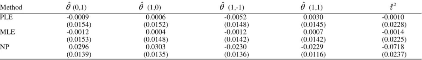
Table 1 shows the simulated bias and simulated standard errrors of the estimated parameters by the three methods for M=64 and Table 2 shows the same information for M=128.
For M=64, the performance of both maximum likelihood and pseudo-likelihood methods is very similar, with only a slight difference in their respective standard deviations. The non-parametric method, based on the window spectral estimate, by contrast, is inferior to these two methods in terms of its bias, though there is little to choose between them in terms of their standard deviations. The bias of the non-parametric method, however, decreases substantially when the lattice size increases to M=128, though the size of this bias is still somewhat larger than that of the maximum likelihood and pseudo-likelihood methods.
Table 3 shows, with M=64,128, the simulated means and standard errors of the estimated index for the three methods. The corresponding theoretical value of the index, AL for the parameterization used here, may
It may be gleaned that the simulated means of the two parametric estimates, even with M=64, are quite close to the theoretical value. The non-parametric estimate of the index, by contrast, is badly biased for M=64. However, for M=128, the bias of the non-parametric estimate is substantially smaller and comparable to that of the two parametric methods. This last result is not surprising since the window spectral estimation method is known to perform relatively poorly with realizations of small lengths.
The simulation results broadly support the model assessment and criticism procedure based on a comparison of the non-parametric and parametric estimates of the index of determinism described earlier. The efficacy of the model validation procedure given was also investigated by an analysis of the residuals
obtained by fitting the full second order model by maximum likelihood and computing the residual correlations. The numerical results are shown in Table 4. It may be seen that the behaviour of the simulated means of the residual correlations accords with the theoretical behaviour described. For the lags included in the set S, the mean residual correlations are quite close to the actual parameter values of the generated model. By contrast, for the lags not included in S, the simulated means are close to 0.
For the same simulated realizations of the second-order model, we also applied the maximum likelihood procedure for fitting three underparametrized models defined as follows:
Table 1: The bias and (standard errors) of the parameter estimates from 1000 simulations of a (64×64) zero mean second order GMRF with toroidal boundary conditions. The true parameters are θ(0,1)=-0.095, θ(1,0)=-0.100, θ(1,1)=-0.092, θ(1,-1)=-0.106 and τ2=1
Method θˆ(0,1) θˆ (1,0) θˆ (1,-1) θˆ (1,1) τˆ2
PLE -0.0009 0.0006 -0.0052 0.0030 -0.0010 (0.0154) (0.0152) (0.0148) (0.0145) (0.0228) MLE -0.0012 0.0004 -0.0012 0.0007 -0.0014
(0.0153) (0.0148) (0.0142) (0.0142) (0.0225) NP 0.0296 0.0303 -0.0230 -0.0229 -0.0718
(0.0139) (0.0135) (0.0136) (0.0116) (0.0237)
Table 2: The bias and (standard errors) of the parameter estimates from 1000 simulations of a (128×128) zero mean second order GMRF with toroidal boundary conditions. The true parameters are θ(0,1)=-0.095, θ(1,0)=-0.100, θ(1,1)=-0.092, θ(1,-1)=-0.106 and τ2=1
Method θˆ(0,1) θˆ (1,0) θˆ (1,-1) θˆ (1,1) τˆ2
PLE 0.0002 0.0003 -0.0029 0.0011 0.0002 (0.0076) (0.0076) (0.0071) (0.0074) (0.0117) MLE 0.0001 0.0001 -0.0008 -0.0005 -0.0001
(0.0075) (0.0073) (0.0068) (0.0070) (0.0116) NP 0.0010 0.0010 -0.0028 -0.0027 0.0007
(0.0075) (0.0075) (0.0069) (0.0068) (0.0115) Table 3: The mean and (standard errors) of the estimated indices of determinism by various methods in 1000 simulations of a (64×64) and
(128×128) zero mean second order GMRF with toroidal boundary conditions. The theoretical value of the index of determinism, AL
for the parameterization used is 0.1359
M PL ML NP
M=64 0.1351 0.1354 0.0721 (0.0151) (0.0148) (0.0129) M=128 0.1351 0.1354 0.1347
(0.0077) (0.0076) (0.0067) Table 4: The mean values of the residual correlations estimated by fitting a (128×128) zero mean second order GMRF with true parameters:
θ(0,1)=-0.095,θ(1,0)=-0.100, θ(1,1)=-0.092, θ(1,-1)=-0.106 and τ2=1
v
Table 5: The means and (standard errors) of the estimated indices of determinism when Models 2, 3 and 4 are fitted to 1000 simulations of Model 1 with M=128; the theoretical value of the index of determinism, AL, for Model 1 is 0.1359
Models PL ML
Model 2 0.0961 0.1149 (0.0073) (0.0084) Model 3 0.1349 0.1351
(0.0077) (0.0076) Model 4 0.1347 0.1348
(0.0077) (0.0076) Table 6: The mean values of the residual correlations estimated by fitting Model 2 to a (128×128) zero mean second order GMRF with true
parameters: θ(0,1)=-0.095, θ(1,0)=-0.100, θ(1,1)=-0.092, θ(1,-1)=-0.106 and τ2=1
v
u --- -4 -3 -2 -1 0 1 2 3 4 4 0.0007 0.0005 -0.0003 0.0015 0.0006 0.0000 0.0001 0.0002 -0.0003 3 0.0001 0.0002 0.0020 0.0018 0.0001 0.0014 0.0013 0.0012 -0.0001 2 -0.0003 0.0009 0.0062 -0.0074 0.0209 -0.0121 0.0096 0.0009 0.0000 1 0.0010 0.0014 -0.0077 0.0971 -0.2233 0.1079 -0.0107 0.0022 0.0005 0 0.0002 0.0007 0.0195 -0.2249 1.0000 -0.2249 0.0195 0.0007 0.0002 -1 0.0005 0.0022 -0.0107 0.1079 -0.2233 0.0971 -0.0077 0.0014 0.0010 -2 0.0000 0.0009 0.0096 -0.0121 0.0209 -0.0074 0.0062 0.0009 -0.0003 -3 -0.0001 0.0012 0.0013 0.0014 0.0001 0.0018 0.0020 0.0002 0.0001 -4 -0.0003 0.0002 0.0001 0.0000 0.0006 0.0015 -0.0003 0.0005 0.0007 Table 7: The mean values of the residual correlations estimated by fitting Model 3 to a (128×128) zero mean second order GMRF with true
parameters: θ(0,1)=-0.095, θ(1,0)=-0.100, θ(1,1)=-0.092, θ(1,-1)=-0.106 and τ2=1
v
u --- -4 -3 -2 -1 0 1 2 3 4 4 0.0007 -0.0001 -0.0005 0.0008 0.0000 -0.0006 -0.0005 0.0000 -0.0007 3 -0.0001 -0.0004 0.0010 0.0002 -0.0007 -0.0012 0.0013 0.0005 -0.0003 2 -0.0007 -0.0002 -0.0011 0.0015 0.0010 -0.0020 0.0001 0.0006 -0.0005 1 0.0005 -0.0001 0.0007 -0.1014 -0.0997 -0.0911 -0.0004 0.0002 -0.0001 0 0.0000 -0.0001 -0.0005 -0.0946 1.0000 -0.0946 -0.0005 -0.0001 0.0000 -1 -0.0001 0.0002 -0.0004 -0.0911 -0.0997 -0.1014 0.0007 -0.0001 0.0005 -2 -0.0005 0.0006 0.0001 -0.0020 0.0010 0.0015 -0.0011 -0.0002 -0.0007 -3 -0.0003 0.0005 0.0013 -0.0012 -0.0007 0.0002 0.0010 -0.0004 -0.0001 -4 -0.0007 0.0000 -0.0005 -0.0006 0.0000 0.0008 -0.0005 -0.0001 0.0007
Table 8: The mean values of the residual correlations estimated by fitting Model 4 to a (128×128) zero mean second order GMRF with true parameters: θ(0,1)=-0.095, θ (1,0)=-0.100, θ (1,1)=-0.092, θ (1,-1)=-0.106 and τ2=1
v
u --- -4 -3 -2 -1 0 1 2 3 4 4 0.0007 -0.0001 -0.0005 0.0008 0.0000 -0.0006 -0.0005 0.0000 -0.0006 3 0.0000 -0.0004 0.0010 0.0002 -0.0006 -0.0012 0.0013 0.0005 -0.0003 2 -0.0007 -0.0002 -0.0012 0.0015 0.0009 -0.0020 0.0001 0.0006 -0.0004 1 0.0005 -0.0001 0.0007 -0.1014 -0.0998 -0.0910 -0.0004 0.0002 -0.0001 0 -0.0001 -0.0001 -0.0006 -0.0947 1.0000 -0.0947 -0.0006 -0.0001 -0.0001 -1 -0.0001 0.0002 -0.0004 -0.0910 -0.0998 -0.1014 0.0007 -0.0001 0.0005 -2 -0.0004 0.0006 0.0001 -0.0020 0.0009 0.0015 -0.0012 -0.0002 -0.0007 -3 -0.0003 0.0005 0.0013 -0.0012 -0.0006 0.0002 0.0010 -0.0004 0.0000 -4 -0.0006 0.0000 -0.0005 -0.0006 0.0000 0.0008 -0.0005 -0.0001 0.0007
Model 2:
[X(s,t 1) X(s,t 1)] ~(1,0)[X(s 1,t) X(s 1,t)] ~(s,t) )
1 , 0 ( ~ ) t , s (
X =−θ − + + −θ − + + +ζ2
Model 3:
[
]
1
2 3
( , ) ( , 1) ( , 1) ( 1, ) ( 1, ) ( 1, 1) ( 1, 1)
( , ) ( 1, 1) ( 1, 1)
X s t X s t X s t X s t X s t
X s t X s t
s t
X s t X s t
θ
θ ζ
= − − + + + − + + +
− − + − + +
− + − + + + + +
ɶ
ɶ ɶ
Model 4:
4
( , ) [ ( , 1) ( , 1) ( 1, ) ( 1, ) ( 1, 1)
( 1, 1) ( 1, 1) ( 1, 1) ( , )
X s t X s t X s t X s t
X s t X s t
X s t X s t
X s t s t
θ
ζ
= − − + + + − +
+ + − − +
+ − + + + −
+ + + +
ɶ
ɶ
where ζɶi( , ), s t i=2,3, 4, denote the theoretical interpolation errors when Model 1 is approximated in a linear least-squares sense by Models 2, 3 and 4, respectively.
one parameter for all four interactions; it thus assumes that the magnitudes of these interactions are equal and the first and second order effects may simultaneously be captured by just one parameter.
Table 5 shows the simulated means and standard errors of the estimated indices, ÂL, in 1000 realizations, each of size M=128, for these three misspecified models. The simulated means for the two isotropic models, Models 3 and 4, are quite close to those shown in Table 3 for the generated Model 1, though the simulated means for Model 4 are slightly smaller than those for Model 3 and this could be because the former uses fewer parameters than the latter. By contrast, for Model 2, the simulated means are noticeably smaller than the non-parametric estimate. The simulation results suggest that, for the parameterization used here, both Models 3 and 4, are probably as effective as the generated second order model with four parameters for describing the spatial correlation structure of the data and for estimating the possible effects of the nearest-neighbours. By contrast, however, the homogeneous first-order model is probably not as effective in capturing the diagonal interactions and it may be improved by choosing either of the two isotropic models or the full second-order model.
The model validation procedure described earlier was also applied to the residuals of Models 2, 3 and 4 by examining the simulated means of their residual correlations. The results are shown in Tables 6, 7 and 8. For Model 2, let S-Z ={(u,v),u,v=±1}, denote the set of sites included in S but excluded from Z={(0,-1),(0,1),(-1,0),(1,0)}. It may be seen that the residual correlations at all lags (u,v) such that (u,v)∈S-Z, are non-negligible, especially relative to their values at lags {(u,v)∉S}. This finding accords with the procedure described in and provides further evidence against adopting Model 2 for data generated from Model 1. By contrast, the residual correlations for both Models 3 and 4 are negligible at lags {(u,v)∉S} and the results provide further evidence that either of these two models may not be excluded as being implausible, even when the observations are generated from Model 1.
The simulation results thus broadly support the three-step procedure suggested in this paper for choosing a suitable GMRF model. This procedure is, however, not a model selection procedure and it does not enable a unique model to be chosen from within the class of models being considered. Rather, it helps in identifying plausible models which could be validly considered as being suitable for the observed data and the final choice among them could well depend upon the actual purpose of the analysis. Further research is nevertheless needed in developing suitable statistical tests for a residual analysis of GMRF and in deriving the sampling distributions of the various measures of linear determinism proposed earlier.
ACKNOWLEDGEMENTS
The research reported in this paper was carried out while Prof. R.J. Bhansali visited the Department of Quantitative Methods and Economic Theory and it was supported by the grant from the University of Chieti-Pescara ’G. d’Annunzio’ for the cooperative agreement between the University of Liverpool and University of Chieti-Pescara.
REFERENCES
1. Bartlett, M.S., 1966. An Introduction to Stochastic
Processes. Cambridge, Cambridge University Press.
2. Whittle, P., 1963. Prediction and Regularization by Linear Least Square Methods. London, English University Press.
3. Brillinger, D.R., 1975. Frequency Analysis of Time Series: Data Analysis and Theory. Holt, Rinehart and Winston, New York.
4. Cleveland, W.S., 1972. The inverse autocorrelations of a time series and their applications. Technometrics, 14: 277-93
5. Chatfield, C., 1979. Inverse autocorrelations. J. Royal Stat. Soc. Ser. A, 142: 363-377.
6. McClave, J., 1978. Estimating the order of moving average models: The Max χ2method. Communication in Statistics, A, 73: 259-276 7. Bhansali, R.J., 1983a. The inverse partial
correlation function of a time series and its applications. J. Mult. Anal., 13: 310-327.
8. Bhansali, R.J., 1983b. Estimation of the order of a moving average model from autoregressive and window estimates of the inverse correlation function. J. Time Ser. Anal., 4: 137-162.
9. Bhansali, R.J., 1987. The discrimination between autoregressive and moving average models from the estimated inverse correlations. Metron, 45: 115-135.
10. Battaglia, F. and R.J. Bhansali, 1987. Estimation of the interpolation error variance and an index of linear determinism. Biometrika, 74: 771-779. 11. Hannan, E.J., 1970. Multiple Time Series. New
York, Wiley.
12. Bhansali, R.J., 1990. On a relationship between the inverse of a stationary covariance matrix and the linear interpolator. J. Appl. Prob., 27: 156-170. 13. Battaglia, F., 1984. Inverse covariances of a
multivariate time series. Metron, 2: 117-129. 14. Masani, P., 1960. The prediction theory of
multivariate stochastic processes, III. Acta Math., 104: 141-162.
15. Rao, C.R., 1973. Linear Statistical Inference and its Applications. New York, Wiley.
17. Bhansali, R.J., 1993. Estimation of the prediction error variance and an R2 measure by autoregressive
model fitting. J. Time Series Anal., 14: 125-146. 18. Hannan, E.J., 1987. Rational transfer function
approximation. Statist. Sci., 2: 1029-1054.
19. Hannan, E.J. and M. Deistler, 1988. The Statistical Theory of Linear Systems. New York, John Wiley and Sons.
20. Akaike, H., 1976. Canonical Correlation Analysis of Time Series and the Use of an Information Criterion. System Identification: Advances and Case Studies, R.K. Mehra and D.G. Lainiotis, eds., New York: Academic Press, pp: 27-96.
21. Barnett, S., 1983. Polynomials and Linear Control Systems. Marcel Dekker. New York.
22. Gohberg, I., P. Lancaster and L. Rodman, 1982. Matrix Polynomials. Academic Press, New York. 23. Kent, J.T. and K.V. Mardia, 1996. Spectral and
circulant approximations to the likelihood for stationary Gaussian random fields. J. Statist. Planning and Inference, 50: 379-394.
24. Yuan, J. and T. Subba Rao, 1993. Spectral estimation for Random Fields with Applications to Markov Modelling and Texture Classification. In Markov Random Fields, Theory and Application, Chellappa, R. and Jain A. Eds., Boston: Academic Press
25. Besag, J.E., 1974. Spatial interaction and the statistical analysis of lattice systems (with discussions). J. Royal Stat. Soc., Series B., 36: 192-236.
26. Besag, J.E. and P.A.P. Moran, 1975. On the estimation and testing of spatial interaction in gaussian lattice processes. Biometrika, 62: 555-562.
27. Box, G.E.P. and G.M. Jenkins, 1970. Time Series Analysis: Forecasting and Control. Holden-Day, San Francisco.
28. Bhansali, R.J., 1981. Effects of not knowing the order of an autoregressive process on the mean squared error of prediction–I. J. Amer. Statist. Assoc., 76: 588-597.
29. Fuller, W.A., 1976. Introduction to Statistical Time Series. New York, John Wiley and Sons, Inc. 30. Kashyap, R.L. and R. Chellappa, 1983. Estimation
and choice of neighbors in spatial-interaction models of images. IEEE Trans. on Information Theory, IT-29: 60-72.
31. Ripley, B.D., 1981. Spatial Statistics. New York: Wiley.
32. Besag, J.E., 1975. Statistical analysis of non-lattice data. The Statistician, 24: 179-195.
33. Dryden, I., L. Ippoliti and L. Romagnoli, 2002. Adjusted maximum likelihood and pseudo-likelihood estimation for noisy gaussian markov random fields. J. Computational and Graphical Statistics, 11: 370-388.