Observed groundwater temperature response to recent climate change

(1)

HESSD

11, 3637–3673, 2014

Groundwater temperature response to climate

change

K. Menberg et al.

Title Page

Abstract Introduction

Conclusions References

Tables Figures

◭ ◮

Back Close

Full Screen / Esc

Printer-friendly Version Interactive Discussion

Discussion

P

a

per

|

D

iscussion

P

a

per

|

Discussion

P

a

per

|

Discuss

ion

P

a

per

|

Hydrol. Earth Syst. Sci. Discuss., 11, 3637–3673, 2014 www.hydrol-earth-syst-sci-discuss.net/11/3637/2014/ doi:10.5194/hessd-11-3637-2014

Hydrology and Earth System

Sciences

Open Access

Discussions

This discussion paper is/has been under review for the journal Hydrology and Earth System Sciences (HESS). Please refer to the corresponding final paper in HESS if available.

Observed groundwater temperature

response to recent climate change

K. Menberg1,2, P. Blum1, B. L. Kurylyk3, and P. Bayer2

1

Karlsruhe Institute of Technology (KIT), Institute for Applied Geosciences (AGW), Karlsruhe, Germany

2

ETH Zurich, Department of Earth Sciences, Zurich, Switzerland

3

University of New Brunswick, Department of Civil Engineering and Canadian Rivers Institute, Fredericton, NB, Canada

Received: 6 February 2014 – Accepted: 28 February 2014 – Published: 28 March 2014

Correspondence to: P. Blum (philipp.blum@kit.edu)

(2)

HESSD

11, 3637–3673, 2014

change

K. Menberg et al.

Title Page

Tables Figures

◭ ◮

Back Close

Full Screen / Esc

Discussion

P

a

per

|

D

iscussion

P

a

per

|

Discussion

P

a

per

|

Discuss

ion

P

a

per

|

Abstract

Climate change is known to have a considerable influence on many components of the hydrological cycle. Yet, the implications for groundwater temperature, as an important driver for groundwater quality, thermal use and storage, are not yet comprehensively understood. Furthermore, few studies have examined the

5

implications of climate change-induced groundwater temperature rise for groundwater-dependent ecosystems. Here, we examine the coupling of atmospheric and groundwater warming by employing stochastic and deterministic models. Firstly, several decades of temperature time-series are statistically analyzed with regard to abrupt climate regime shifts (CRS) in the long-term mean. The observed abrupt

10

increases in shallow groundwater temperatures can be associated with preceding positive shifts in regional surface air temperatures, which are in turn linked to global air temperature changes. The temperature data are also analyzed with an analytical solution to the conduction-advection heat transfer equation to investigate how subsurface heat transfer processes control the propagation of the surface

15

temperature signals into the subsurface. In three of the four monitoring wells, the predicted groundwater temperature increases driven by the regime shifts at the surface boundary condition generally concur with the observed groundwater temperature trends. Due to complex interactions at the ground surface and the heat capacity of the unsaturated zone, the thermal signals from distinct changes in air temperature

20

are damped and delayed in the subsurface, causing a more gradual increase in groundwater temperatures. These signals can have a significant impact on large-scale groundwater temperatures in shallow and economically important aquifers. These findings demonstrate that shallow groundwater temperatures have responded rapidly to recent climate change and thus provide insight into the vulnerability of aquifers and

25

(3)

HESSD

11, 3637–3673, 2014

change

K. Menberg et al.

Title Page

Tables Figures

◭ ◮

Back Close

Full Screen / Esc

Discussion

P

a

per

|

D

iscussion

P

a

per

|

Discussion

P

a

per

|

Discuss

ion

P

a

per

|

1 Introduction

Atmospheric climate change is expected to have a significant influence on subsurface hydrological and thermal processes (e.g. Bates et al., 2008; Green et al., 2011; Gunawardhana and Kazama, 2012). While the consequences for groundwater recharge and water availability were scrutinized by many studies (e.g. Maxwell and

5

Kollet, 2008; Ferguson and Maxwell, 2010; Stoll et al., 2011; Taylor et al., 2013; Kurylyk and MacQuarrie, 2013a), the implications of changing climate conditions for the long-term evolution of shallow groundwater temperatures are not comprehensively understood (Kløve et al., 2013). Groundwater temperature (GWT) is known to be an important driver for water quality (e.g. Green et al., 2011; Sharma et al., 2012; Hähnlein

10

et al., 2013) and therefore, it is a crucial parameter for groundwater resource quality management (Figura et al., 2011).

Furthermore, increasing groundwater temperatures can have a significant influence on groundwater and river ecology (e.g. Kløve et al., 2013). Numerous studies on the impact of recent or projected climate change on the thermal regimes of surface

15

water bodies and the associated impact for coldwater fish habitats have already been conducted (e.g. Kaushal et al., 2010; van Vliet et al., 2011; van Vliet et al., 2013; Wenger et al., 2011; Isaak et al., 2012; Wu et al., 2012; Jones et al., 2014), but the thermal sensitivity of shallow aquifers to climate change is a relatively unstudied phenomenon (e.g. Brielmann et al., 2009, 2011; Taylor and Stefan, 2009; Kurylyk et al.,

20

2013). The thermal response of GWT to climate change is of particular interest to river temperature analysts, as the thermal regimes of baseflow-dominated streams or rivers and hydraulically connected aquifers are inextricable linked (Hayashi and Rosenberry, 2002; Tague et al., 2007; Risley et al., 2010). Furthermore, groundwater-sourced coldwater plumes within river mainstreams are known to provide thermal

25

(4)

HESSD

11, 3637–3673, 2014

change

K. Menberg et al.

Title Page

Tables Figures

◭ ◮

Back Close

Full Screen / Esc

Discussion

P

a

per

|

D

iscussion

P

a

per

|

Discussion

P

a

per

|

Discuss

ion

P

a

per

|

lack of knowledge regarding the thermal vulnerability of GWT to climate change and the associated impacts to GDEs has been highlighted as a research gap in several recent studies (e.g. Bertrand et al., 2012; Mayer, 2012; Kanno et al., 2013).

Thermal signals arising from changes in ground surface temperatures (GST) propagate downward into the subsurface, causing GWT to deviate from the undisturbed

5

geothermal gradient. Heat transport theory has been applied for inverse modeling of temperature-depth profiles to infer paleoclimates based on measured deviations from the geothermal gradient (e.g. Mareschal and Beltrami, 1992; Pollack et al., 1998; Beltrami et al., 2006; Bodri and Cermak, 2007) and for forward modeling the impact of projected climate change on measured temperature-depth profiles (e.g.

10

Gunawardhana and Kazama, 2011; Kurylyk and MacQuarrie, 2013b). Such studies are often based on the assumption that long term trends in GST will track long term trends in surface air temperature (SAT), although this has been a matter of considerable debate (e.g. Mann and Schmidt, 2003; Chapman et al., 2004; Schmidt and Mann, 2004). For example, decreases in the duration of thickness of the insulating winter

15

snowpack due to rising SAT can paradoxically lead to decreased winter GST (Smerdon et al., 2004; Zhang et al., 2005; Mellander et al., 2007; Mann et al., 2009; Kurylyk et al., 2013), which lead to a decoupling of mean annual SAT and GST trends. Likewise, variations in incident solar radiation were shown to perturb the surface energy balance in a way that contradicts the assumptions of vertical conductive heat transport (Beltrami

20

and Kellman, 2003). Furthermore, Lesperance et al. (2010) show that the relationship between SAT and subsurface temperature development over intervals of several years to decades is also strongly impacted by the annual variability of SAT. Thus, equivalent trends in SAT and shallow subsurface temperatures are not sufficient to characterize their long-term relationship.

25

(5)

HESSD

11, 3637–3673, 2014

change

K. Menberg et al.

Title Page

Tables Figures

◭ ◮

Back Close

Full Screen / Esc

Discussion

P

a

per

|

D

iscussion

P

a

per

|

Discussion

P

a

per

|

Discuss

ion

P

a

per

|

solutions have been proposed that account for subsurface thermal perturbations arising from a combination of climate change and vertical groundwater flow (e.g. Taniguchi et al., 1999a, b; Kurylyk and MacQuarrie, 2013b). The solutions vary depending on the nature of the surface boundary conditions employed (e.g. linear, exponential, or step trends in temperature), which can be used to match measured or predicted GST

5

trends for a region. These solutions do not account for horizontal groundwater flow, which can also perturb subsurface thermal regimes in certain environments (Ferguson and Bense, 2011; Saar, 2011).

Figura et al. (2011) show that temperature variations in Swiss aquifers that are recharged by river water through bank infiltration can be related to changes in climate

10

oscillations systems by applying a statistical regime shift analysis. Characterizing changes in time-series of various climatic, physical and biological parameters with the concept of abrupt regime shifts has been the focus of numerous studies in the last two decades (e.g. Hare and Mantua, 2000; Overland et al., 2008). In this context, a regime is often defined as a period with stable behaviour or with a quantifiable

quasi-15

equilibrium state (deYoung et al., 2004), and accordingly a rapid transition between states with di_ffering average characteristics over multi-annual to multi-decadal periods is referred to as a regime shift (Bakun, 2004).

In this study, we demonstrate the direct influence of atmospheric temperature development on shallow GWT at two sites in Germany by analyzing time-series of SAT

20

and GWT with regard to abrupt changes in the long-term annual mean. Furthermore, we compare different spatially averaged temperature time-series from individual weather stations to global mean air temperature change bringing our observations in the context of global climate change. The magnitudes of the regime shifts and the time lags between the shifts in the chosen time-series are evaluated under consideration of

25

(6)

HESSD

11, 3637–3673, 2014

change

K. Menberg et al.

Title Page

Tables Figures

◭ ◮

Back Close

Full Screen / Esc

Discussion

P

a

per

|

D

iscussion

P

a

per

|

Discussion

P

a

per

|

Discuss

ion

P

a

per

|

2 Data and methods

2.1 Data and site description

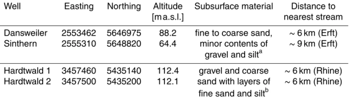
For the analysis of shallow GWT, we use time-series from four observation wells in porous and unconfined aquifers in Germany (Table 1, Fig. 1a and b). Two of the wells are installed in the surrounding area of Cologne outside the small villages of

5

Dansweiler and Sinthern in agricultural areas. The other two wells are located in a rather densely vegetated forest, called Hardtwald, close to the city of Karlsruhe and are therefore named Hardtwald 1 and 2. The proximate surroundings of all four wells were undisturbed over the last decades, so that variations in GWT due to land use changes are unlikely. The distances from the observation wells to the nearest stream

10

are several kilometers (Table 1), thus the influence of river water on the groundwater temperature in the wells can be excluded.

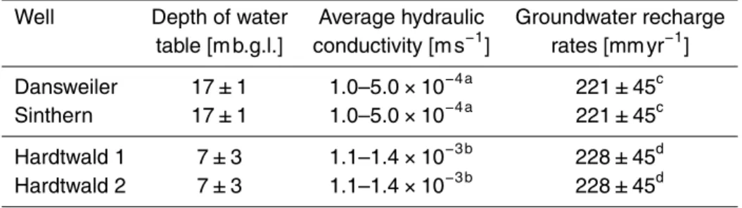
Table 2 lists some basic hydrogeological properties of the studied aquifers. The depth of water table differs considerably between the two well fields, with around 17 m for the Cologne aquifer and about 7 m near Karlsruhe. Variations in the depth of water table

15

during the observation period are within 2 m for the Dansweiler and Sinthern wells and more pronounced in the Hardtwald wells with about 6 m. Both aquifers are recharged by infiltration of meteoric water through the unsaturated zone with estimated recharge rates of 221±45 mm yr−1 for the Cologne aquifer and 228±45 mm yr−1 for the aquifer

near Karlsruhe (Table 2).

20

A schematic cross-section of the two aquifers near Cologne (left) and Karlsruhe (right) in Fig. 1c and d shows the average depth of the water table below surface level and the depth of the underlying aquitard. Details on the wells’ constructions are also depicted with the overall depth and the locations of the filter screens (black areas) that indicate the depth where the pumped water is captured. Furthermore, Fig. 1c and d

25

(7)

HESSD

11, 3637–3673, 2014

change

K. Menberg et al.

Title Page

Tables Figures

◭ ◮

Back Close

Full Screen / Esc

Discussion

P

a

per

|

D

iscussion

P

a

per

|

Discussion

P

a

per

|

Discuss

ion

P

a

per

|

GWT in all observations wells was measured one to six times per year for a period of at least 32 years (1974–2006) during frequent water quality assessments by the local groundwater authorities. During the specified procedure, water is pumped from the wells until the water temperature and other on-site parameters are constant. The temperature measurements are thereby conducted with a probe directly at the outlet,

5

before it can equilibrate with the surrounding air temperature. Thus, the temperature can be seen as representative annual means for the upper part of the aquifers, as indicated by the well screens in Fig. 1c and d. If two or more GWT measurements were available per year, the arithmetic mean is adopted as the annual mean value.

Annual SAT data are available from weather stations operated by the German

10

Weather Service (DWD) outside the cities of Cologne and Karlsruhe in agricultural surroundings (Fig. 1a and b). Though located several kilometers from the observation wells, the SAT from these stations is expected to yield a good approximation for the development of SAT at the well sites. Furthermore, for the evaluation of abrupt shifts in the time series of SAT and GWT, the absolute temperature is only of minor importance,

15

while the main focus is on the timing of the shifts and the temperature differences. For the comparison with air temperatures on a larger scale, we use time-series of mean air temperature anomalies based on the reference period 1951–1980 from the NASA Goddard Institute for Space Studies (GISS) (e.g Hansen et al., 2010). Of the spatially averaged temperature data sets available, we evaluate the annual global mean from

20

land-surface air and sea-surface water temperature anomalies and the annual zonal mean for the Northern Hemisphere between 90 and 24◦N based on land-surface air temperature anomalies.

2.2 Regime shift analysis

There are several possibilities to statistically evaluate temperature changes in time

25

(8)

HESSD

11, 3637–3673, 2014

change

K. Menberg et al.

Title Page

Tables Figures

◭ ◮

Back Close

Full Screen / Esc

Discussion

P

a

per

|

D

iscussion

P

a

per

|

Discussion

P

a

per

|

Discuss

ion

P

a

per

|

using breakpoints than by models assuming monotonic functions. Hence, we here apply a sequentialt-test analysis for regime shifts (STARS) to detect possible abrupt regime shifts (CRS) in the temperature time-series (Rodionov, 2004; Rodionov and Overland, 2005). The STARS method has been successfully used by recent studies to identify abrupt changes in the long-term mean of environmental time-series (Marty,

5

2008; Figura et al., 2011; North et al., 2013). STARS is a parametric test that can detect multiple regime shifts and needs no a priori assumption for the timing of possible shifts. Identification of a shift is based on the calculation of the Regime Shift Index (RSI), which represents the cumulative sum of the normalized deviations from the mean value of a regime and thus reflects the confidence of a regime shift (Rodionov,

10

2004). For the regime shift analysis, several test parameters can be adjusted to account for specific characteristics, such as the length of the tested time-series. The target significance level in our analysis is set to 0.15, which corresponds to the p-level of false positives. The actualpvalue of an identified shift between subsequent regimes is calculated separately with a Student’st test. The cut-offlength of the test corresponds

15

to a low-pass filter, so that regimes with a shorter length are disregarded in the analysis (Rodionov and Overland, 2005). Here, we set the cut-o_ff length to 10 years as atmospheric oscillations often occur at decadal intervals (Overland et al., 2008). Furthermore, the Huber weight parameter (set to 1 in our study) included in the STARS procedure improves the treatment of outliers by weighting them proportionally to their

20

deviation from the mean value (Overland et al., 2008). As pointed out by Seidel and Lanzante (2004) atmospheric data tend to be highly temporally auto-correlated, so that especially in short time series, spurious regime shifts may be detected due to serial correlation (Rudnick and Davis, 2003). Therefore, we apply a pre-whitening procedure that removes the red noise component from the temperature time series prior to testing

25

(9)

HESSD

11, 3637–3673, 2014

change

K. Menberg et al.

Title Page

Tables Figures

◭ ◮

Back Close

Full Screen / Esc

Discussion

P

a

per

|

D

iscussion

P

a

per

|

Discussion

P

a

per

|

Discuss

ion

P

a

per

|

2.3 Analytical solutions

The governing equation often employed for transient subsurface heat transport is the one dimensional conduction equation for homogeneous media, which equates the divergence of the conductive flux with the rate of the change of thermal energy in the medium (Carslaw and Jaeger, 1959; Domenico and Schwartz, 1990):

5

κ∂

2

T ∂z2 =

∂T

∂t (1)

where κ is the bulk thermal diffusivity of the subsurface (m2s−1), T is temperature (◦C),z is depth (m), andtis time (s). The governing heat transport equation becomes slightly more complex when advective heat transport (or “forced convection”) due to groundwater flow is considered:

10

κ∂

2

T ∂z2−U

∂T ∂z =

∂T

∂t (2)

whereU (m s−1) is a function of the Darcy velocityq(downwards is positive, m s−1), the bulk volumetric heat capacity of the soil-water matrixC(J m−3◦_C−1_{), and the volumetric}

heat capacity of waterC_w(J m−3◦C−1):

U₌qCw

C (3)

15

Here we employ a distinct analytical solution to Eq. (2) to simulate the influence of a climate regime shift on GWT. We assume thermally uniform initial conditions and boundary conditions that are subject to a series ofnstep increases in GST:

initial conditions: T(z,t₌0)=T₀ (4)

boundary condition: T(z₌0,t)₌T₀₊ n X

i=1

∆GST_i·H(t−ti) (5)

(10)

HESSD

11, 3637–3673, 2014

change

K. Menberg et al.

Title Page

Tables Figures

◭ ◮

Back Close

Full Screen / Esc

Discussion

P

a

per

|

D

iscussion

P

a

per

|

Discussion

P

a

per

|

Discuss

ion

P

a

per

|

where T₀ is the initial uniform temperature (◦_{C) prior to the beginning of the regime}

shift, ∆GSTi is the step increase in GST for regime shift i (◦C), H is the Heaviside

step function, and t_i is the time (s) of the beginning of regime shift i. In this formulation, _∆GST_i refers to a step change in GST in comparison to the GST conditions immediately preceding that change (not necessarily in comparison to initial

5

GST,T₀). We ignore short term (e.g. annual) variations in SAT and GST and rather drive the subsurface heat transport models with temperatures averaged for a given climate regime and then instantaneously increased at the beginning of the next climate regime. The thermally uniform initial conditions is a reasonable assumption given that we begin by considering mean annual GWT at or near the water table following a relatively

10

stable climate regime (i.e. prior to 1988, Fig. 2). Moreover, for the wells observed, the vadose zones and near-surface aquifers are too shallow to realize the influence of any geothermal gradient.

The transient conduction-advection heat transport model (TCA model) employed in this study is an analytical solution to the transient conduction-advection Eq. (2)

15

subject to the initial and boundary conditions given in Eqs. (4) and (5). This solution was originally developed by Carslaw and Jaeger (1959) and subsequently employed by Taniguchi et al. (1999b) to study subsurface temperature evolution in regions of significant groundwater flow. Because we assume initially thermally uniform conditions in the unsaturated zone and shallow groundwater, the resultant solution is simpler than

20

(11)

HESSD

11, 3637–3673, 2014

change

K. Menberg et al.

Title Page

Tables Figures

◭ ◮

Back Close

Full Screen / Esc

Discussion

P

a

per

|

D

iscussion

P

a

per

|

Discussion

P

a

per

|

Discuss

ion

P

a

per

|

differential equation and the boundary and initial conditions (Farlow, 1982):

T(z,t)=T₀₊ n X

i=1

∆GST_i 2

(

erfc z−U(t−ti) 2pκ(t₋t_i)

!

+exp

_U z κ

erfc z+U(t−ti) 2pκ(t₋t_i)

!)

·H(t−ti)

(6)

whereT(z,t) is the spatiotemporally varying subsurface temperature (GWT,◦C), κ is the bulk thermal diffusivity of the subsurface (m2s−1), and erfc is the complementary

5

error function. Comparisons between the model results and measured GWT indicate whether these simple analytical solutions are applicable for modeling the influence of observed and projected climate regime shifts in the wells considered in this study.

It should be noted that it is the GST rather than the SAT that drives subsurface thermal regimes and thus forms the boundary condition in Eq. (5). However, complete

10

GST time series were not available for the locations considered in this study. Thus, in the present study, the magnitude and timing of the regime shifts in GST are obtained from the SAT data as follows. In all cases, the timing of the GST regime shifts is assumed to correspond to the timing of the SAT regime shifts for that location obtained from the statistical analysis. This approach is reasonable given the efficient heat

15

transfer that occurs between the lower atmosphere and the ground surface (e.g. Bonan, 2008). For the open, agricultural site near Cologne (wells Dansweiler and Sinthern, Table 2) the magnitude of the GST regime shift was set to be equal to the magnitude of the SAT regime shift as determined from the statistical analysis. Measured SAT and GST data (not shown) indicate that this approach is valid in the open sites as the

20

measured magnitude of the climate regime shift in 1988 was 1.1◦C in both the SAT and GST data. However, in the forested sites (Hardtwald 1 and 2, Table 2), for which measured GST were not available, the influence of the vegetative canopy can decouple GST and SAT regime shifts. For example, under a deciduous canopy, the length of the growing season (and thus the shading influence of the forest canopy) is increased in

(12)

HESSD

11, 3637–3673, 2014

change

K. Menberg et al.

Title Page

Tables Figures

◭ ◮

Back Close

Full Screen / Esc

Discussion

P

a

per

|

D

iscussion

P

a

per

|

Discussion

P

a

per

|

Discuss

ion

P

a

per

|

a warmer climate (Bonan, 2008). Zhang et al. (2005) conducted a detailed study of the relationship between GST and SAT changes in the twentieth century in Canada and found that, on average, GST changes were 60 % of air temperature changes. Much of this study was conducted for forested sites with seasonal snow cover. Hence, in this study, we test two assumptions for the magnitude of the GST regime shifts in the

5

forested sites:

∆GSTi = ∆SATi (7)

∆GSTi =0.6×∆SATi (8)

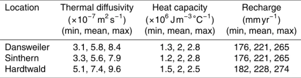
Table 3 presents the assumed subsurface thermal properties for each well. A potential

10

range in these values was estimated from drilling logs and respective literature values based on the lithology and variability in water saturation (VDI, 2010; Menberg et al., 2013). Regional recharge rates were extracted from Table 2 with a potential range to reflect the variability of recharge in this region (Erftverband, 1995; W. Deinlein, personal communication, 2013). Similar thermal properties and recharge values are assumed

15

for Hardtwald 1 and Hardtwald 2 based on their similar land cover and subsurface properties and the geographical proximity (about 200 m) between the wells.

3 Results and discussion

3.1 Statistical analysis

3.1.1 Regime shifts in air and groundwater temperatures

20

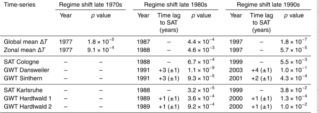
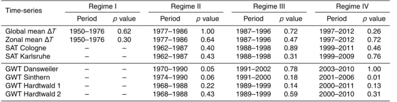
At least two climate regime shifts (CRS) could be detected in the later decades of all analyzed time-series (Fig. 2). The time-series of global mean temperature change and zonal mean temperature change in 90–24◦N show significant (STARS,p <0.005) positive shifts in 1977, 1987, 1997 and 1977, 1988 and 1998, respectively (Table 4). The observation of shifts in air temperature change in these years is in good agreement

(13)

HESSD

11, 3637–3673, 2014

change

K. Menberg et al.

Title Page

Tables Figures

◭ ◮

Back Close

Full Screen / Esc

Discussion

P

a

per

|

D

iscussion

P

a

per

|

Discussion

P

a

per

|

Discuss

ion

P

a

per

|

with the observation of decadal shift in atmospheric oscillation indices in the late 1970s, late 1980s and late 1990s (Overland et al., 2008). Only the CRS in the late 1980s and late 1990s can be found from examining the time-series of local SAT data from Cologne and Karlsruhe. However, this is not surprising as previous studies observed that the CRS in the late 1970s was most prominent in the North Pacific region (Hare

5

and Mantua, 2000; Overland et al., 2008), and less accentuated in Europe. The same applies to the CRS in the late 1990s (Overland et al., 2008; Swanson and Tsonis, 2009), which is reflected by the differing RSI values in Fig. 2. While the high RSI for the CRS in 1997 in the global mean temperature change indicates a significant shift, the RSIs for the late 1990s CRS in the German SAT time-series are much lower than

10

the RSIs in the late 1980s. Figura et al. (2011) correlated the abrupt increase in SAT in Switzerland with a change in the Artic Oscillation (AO) that has a strong influence on air temperatures in Europe. However, no such change in the AO Index was found in the late 1990s, suggesting that the CRS in the German SAT is also coupled to the general air temperature increase in the Northern Hemisphere.

15

Two regime shifts were detected in the GWT time-series for the four wells near Cologne and Karlsruhe. These shifts correspond to the CRS in the atmosphere with a certain time lag (Fig. 2, Table 4). The regime shifts in GWT time-series are all statistically significant (p <0.01), except for the second regime shift in the late 1990s in Dansweiler. Two prominent outliers in the third regime of the time series

20

influence the statistical significance for this shift, while the RSI value is calculated under consideration of the outliers according to the Huber weight parameter. Furthermore, the RSI values in Fig. 2 for the second shifts in Dansweiler and Sinthern are not the final values, as the 10-year cut-offlength of the STARS test in the last regime has not yet been reached. In general, the time series of GWT show a more gradual increase

25

(14)

HESSD

11, 3637–3673, 2014

change

K. Menberg et al.

Title Page

Tables Figures

◭ ◮

Back Close

Full Screen / Esc

Discussion

P

a

per

|

D

iscussion

P

a

per

|

Discussion

P

a

per

|

Discuss

ion

P

a

per

|

to the fact the pumped groundwater from the Hardtwald wells contains water from quite shallow depths (Fig. 1c and d), where temperature is strongly influenced by variations in SAT. Gosnold et al. (1997) and Lesperance et al. (2010), amongst others, also noted the fact that temperatures in the subsurface up to 30 m can show significant annual variability due to the inter-annual variability of air and ground temperature.

5

3.1.2 Statistical analysis of time lags and magnitude of temperature change

The time lags between the regime shifts in SAT and GWT are listed in Table 4. The regime shifts in global mean temperature change and the zonal mean in 90–24◦_{N occur}

simultaneously, except for the regime shift in the late 1980s that has a time lag of one year. However, as annual mean values are used for the analysis, the accuracy of the

10

shift detection is limited to±1 year, so that the shifts occur within the uncertainty range.

The same applies to the first regime shifts in the local SAT time-series in Cologne and Karlsruhe, while the time lag of 2 years in the second shift is significant. A possible explanation for this variation in the time lags would be that the late 1980s regime shift was very prominent in the Arctic Oscillation that directly influences the European

15

climate (Figura et al., 2011). The late 1990s regime shift however, was more distinct in the North Pacific region (Overland et al., 2008), thus probably causing the delayed shift in the SAT in Germany. Yet, changes in SAT are also expected to be temporally and spatially highly heterogeneous due to the variability of local climate and the complexity of atmospheric circulation systems (Hansen et al., 2010).

20

The observed CRS in shallow GWT lag behind the abrupt increase in local SAT by 1–4 years (Table 4). In Karlsruhe the time lag is generally small with one year for all shift events, while the time lags in Cologne vary between 2–4 years. This difference in the time lags reflects the specific hydrogeological site conditions with the unsaturated zone in Cologne (17 m) being significantly thicker than in Karlsruhe (7 m, Table 2).

25

(15)

HESSD

11, 3637–3673, 2014

change

K. Menberg et al.

Title Page

Tables Figures

◭ ◮

Back Close

Full Screen / Esc

Discussion

P

a

per

|

D

iscussion

P

a

per

|

Discussion

P

a

per

|

Discuss

ion

P

a

per

|

measurements, and ocean temperatures are known to respond more slowly to climatic forcing due to the ocean’s large thermal inertia (Hansen et al., 2010). The above mentioned temporal and spatial heterogeneity of the CRS accounts also for the higher increase in SAT in the German time series, which is above the average of the zonal mean in 90–24◦N. The significant abrupt increase in the long-term mean of SAT with

5

the late 1980s CRS of close to 1◦C was likewise observed in Swiss SAT by Figura et al. (2011).

The magnitudes of the abrupt increases in the long-term means of GWT are lower and damped by up to 70 % compared to the shift magnitude in SAT (Fig. 3). This damping arises from the fact that, due to the thermal inertia of the subsurface, the

10

GWT has not yet fully equilibrated with the GST at the time when the regime shift is observed in the GWT. The magnitudes of the regime shifts in Fig. 3 also reveal that the damping in in the time-series from the Hardtwald wells is more pronounced than the damping in Dansweiler and Sinthern. As aforementioned, the evolution of subsurface temperatures is driven by the GST and site-specific parameters. The assumption,

15

that GST changes closely track changes in SAT, which is commonly applied for past climate reconstructions from borehole temperatures, has been controversly discussed in literature (e.g. Mann and Schmidt, 2003; Chapman et al., 2004; Schmidt and Mann, 2004). Our observations of differing magnitudes in atmospheric and subsurface warming seem to support the presumption that, at least for the forested

20

site with shallow wells (and thus short lags), subsurface temperatures are not perfectly coupled to evolution of regional SAT in recent rapid climate change. The ground heat flux, i.e. the part of the energy budget at the ground surface that propagates from the atmosphere into the subsurface, depends also on surface and atmospheric parameters. As the wells near Karlsruhe are located in a forest and the wells near

25

(16)

HESSD

11, 3637–3673, 2014

change

K. Menberg et al.

Title Page

Tables Figures

◭ ◮

Back Close

Full Screen / Esc

Discussion

P

a

per

|

D

iscussion

P

a

per

|

Discussion

P

a

per

|

Discuss

ion

P

a

per

|

3.1.3 Stationarity within the regimes

In order to investigate the stationarity within the identified regimes the Mann–Kendall test for the absence of trend was performed for the individual regimes. The resulting

p values are listed in Table 5, in which high p values close to 1 indicate stationary conditions. No significant trends could be found within the individual regimes of

5

the examined SAT time-series, suggesting that the temperature increase in the last decades can be attributed completely to the detected CRS. In the GWT time series, a significant trend (p <0.05) with a slope of 0.13◦C was detected in the third regime (2001–2006) in the Sinthern well. However, it has to be noted, that this regime is quite short, and thus the trend analysis may be biased by the last two rather high temperature

10

values in 2005 and 2006. In the regimes before 1991, thepvalues of the time-series in Dansweiler and Sinthern are 0.05 and 0.06, respectively, and thus close to the critical

pvalue of 0.05 suggesting the possibility of a more gradual increase. For the wells near Karlsruhe no significant trends were found in GWT within the regimes, which indicates that the temperature increase in the time series can be completely linked to the regime

15

shifts. However, detailed inspection of thep values of the Mann–Kendall test reveals that the SAT time series yield higher p values (median of 0.53) than the GWT time series (median of 0.20, Table 5), indicating that the SAT time series are generally more stationary than GWT time series.

To compare the performance of the regime shift analysis to an approach with linear

20

temperature increase, the RMSE values for the statistical step function model and a linear model were calculated for each time series (not shown). This analysis revealed that the RMSE of the step function fit for all GWT and SAT time series is slightly lower than the RMSE of the linear fit, indicating that the step function model performs slightly better. Thus, it can be stated, that, with the exception of the potentially biased last

25

(17)

HESSD

11, 3637–3673, 2014

change

K. Menberg et al.

Title Page

Tables Figures

◭ ◮

Back Close

Full Screen / Esc

Discussion

P

a

per

|

D

iscussion

P

a

per

|

Discussion

P

a

per

|

Discuss

ion

P

a

per

|

3.2 Analytical model

Predicted GWT were obtained from the analytical solution in Eq. (6) (TCA model) with the thermal properties and recharge rates given in Table 3 and the magnitude and timing of the regime shifts given in Table 4. Due to the availability of GWT data in each well, model runs were started in 1970. It should be noted that predicted GWT results

5

obtained with the analytical solution represent the temperature at the (ground)water table (i.e. thezterm in Eq. (6) is set to the groundwater table depth). The well screens are, of course, somewhat below the water table (Fig. 1); however, due to the cone of depression in the groundwater capture zone (Domenico and Schwartz, 1990), the extracted water would primarily come from depths close the water table. Furthermore,

10

the GWT close to the well is relatively uniform during pumping given the high heat advection and concomitant thermal dispersion.

Figure 4 shows the measured GWT, assigned GST boundary condition, and predicted GWT for each of the four wells. The range of predicted GWT (shaded area, Fig. 4) is derived from the range of thermal properties and recharge values utilized

15

as input parameters to the model (Table 3). Note that the GST data simulated for the deeper wells (Sinthern and Dansweiler) is more sensitive to the selection of the thermal properties than the shallower wells. This is because deeper wells require more time to equilibrate with the GST regime shifts, and they are therefore more sensitive to the magnitude of the conductive and advective heat flux. Hereafter, when we refer to the

20

TCA model results we ignore the range in the modeling results and only allude to the specific results obtained using the mean recharge values and mean thermal properties given in Table 3 (i.e. red series, Fig. 4).

The TCA model predicted trends in GWT concur with the general trends exhibited in the measured data for Dansweiler; however, the TCA model under-predicts the rise in

25

(18)

HESSD

11, 3637–3673, 2014

change

K. Menberg et al.

Title Page

Tables Figures

◭ ◮

Back Close

Full Screen / Esc

Discussion

P

a

per

|

D

iscussion

P

a

per

|

Discussion

P

a

per

|

Discuss

ion

P

a

per

|

greater than the obtained regional recharge rates for this area. Higher recharge would lead to higher heat advection, which would reduce the lag between a GST signal and its realization in the subsurface (see range in predicted Sinthern GWT, Fig. 4). Similarly, higher thermal diffusivity would generally lead to higher GWT in Sinthern, as the Sinthern GWT is still adjusting to the GST regime shifts in the data shown in Fig. 4.

5

Finally, the last few years of measured GWT data are not available for the Sinthern well. GWT data in the nearby Dansweiler well decreased during this period, thus the visual fit between the measured and predicted Sinthern GWT would likely improve if these data were available.

The solid red lines in Fig. 4, which represent the results obtained by assuming

10

∆GST_{= ∆}SAT (Eq. 7), exceed the measured GWT data for this period in the Hardtwald wells (RMSE=0.43◦C). This suggests that GST regime shifts are damped in comparison to the SAT regime shifts in forested sites. The series produced by assuming _∆GST₌0.6·∆SAT (Eq. 8) are in better agreement (RMSE₌0.26◦_{C) with}

the measured GWT, and thus these results concur with the relationship between∆GST

15

and∆SAT previously simulated by Zhang et al. (2005).

Our approach does not reproduce annual variability in GWT due to the nature of the GST boundary condition, which is constant for a given climate regime (Fig. 4). Annual variability in GWT could theoretically be reproduced by considering a series of “GST regimes” that only last one year; however, the objective of the present study was to

20

examine the subsurface thermal influence of climate regime shifts not inter-annual SAT or GST variability.

Finally, it is interesting to note that the abrupt regime shifts applied in the simplified boundary condition manifest themselves as gradual changes in the predicted GWT evolution in the deeper wells due to the influence of the heat capacity and thermal

25

(19)

HESSD

11, 3637–3673, 2014

change

K. Menberg et al.

Title Page

Tables Figures

◭ ◮

Back Close

Full Screen / Esc

Discussion

P

a

per

|

D

iscussion

P

a

per

|

Discussion

P

a

per

|

Discuss

ion

P

a

per

|

predicted and observed trends in GWT data (Fig. 4) indicates that TCA model can produce first-order approximations of the thermal sensitivity of these shallow aquifers to past or future climate regime shifts.

3.2.1 Implications for future river temperatures and groundwater-dependent

ecosystems 5

Although the wells analysed in this study were not located nearby streams, the timing and magnitude of the measured GWT rise can provide insight into the potential warming of alluvial aquifers feeding ecologically important rivers. Gaining rivers and streams can be strongly influenced by the thermal regimes of surrounding aquifers (e.g. Tague et al., 2007; Kelleher et al., 2012), and this is often particularly true

10

during the dry, warm season when baseflow can provide the majority of the river or stream discharge. Thus, deterministic models of future base-flow dominated rivers temperature should explicitly account for the future thermal regimes of aquifers. Various studies have demonstrated that the thermal regimes of rivers respond to a warming climate, and these studies have generally either tacitly ignored GWT rise due to

15

climate change (citing potential lags of centuries) or assumed GWT warming is actually equivalent in magnitude to SAT warming. The results of this study however contradict both of these assumptions by indicating that GWT warming are likely be damped in comparison to SAT warming and that the lag time between SAT warming and the associated increase in shallow GWT can be rather short (<5 years). Similar results

20

were obtained by Kurylyk et al. (2014) who employed a numerical model of groundwater flow and energy transport driven by downscaled climate scenarios to demonstrate a potential damping and short lagging of future groundwater temperature rise in response to air temperature changes.

Given the expected warming of rivers across the globe (van Vliet et al., 2011, 2013),

25

(20)

HESSD

11, 3637–3673, 2014

change

K. Menberg et al.

Title Page

Tables Figures

◭ ◮

Back Close

Full Screen / Esc

Discussion

P

a

per

|

D

iscussion

P

a

per

|

Discussion

P

a

per

|

Discuss

ion

P

a

per

|

warm in response to climate change. The magnitude and timing of the GWT warming however will depend on several factors, including the timing and magnitude of the SAT warming, changes in precipitation (and thus recharge and advection), the depth of the groundwater table, and the presence or absence of seasonal snowpack and vegetation canopy.

5

4 Conclusions

By applying a sequential t-test analysis for regime shifts (STARS) to time-series of air and groundwater temperatures, we empirically demonstrated that groundwater temperatures in shallow aquifers show abrupt temperature changes that correspond to positive shifts in local SAT in Germany, which in turn can be traced back to increasing

10

global SAT. This observed direct coupling of atmospheric and groundwater temperature development through the unsaturated zone implies that climate warming does not only affect aquifers recharged by river-bank infiltration (Figura et al., 2011), but also a large number of shallow aquifers on a wide spatial scale. The regime shifts in GWT occur with a certain time lag to the CRS depending mainly on the thermal properties and thickness

15

of the unsaturated zone. The magnitude of these regime shifts in GWT compared to the shifts in SAT is damped by the thermal propagation of the temperature signal into the subsurface, leading to a more gradual increase in GWT. However, despite the extenuation of the temperature signal in the subsurface and the mixing of shallow groundwater during pumping, significant temperature shifts were found in the extracted

20

groundwater.

Process-oriented modeling was also performed with an analytical solution to the conduction-advection equation. In three of the four observation wells, the simulated decadal GWT trends generally concurred with the measured decadal GWT trends, although annual variability was not reproduced due to the simplistic nature of the

25

(21)

conduction-HESSD

11, 3637–3673, 2014

change

K. Menberg et al.

Title Page

Tables Figures

◭ ◮

Back Close

Full Screen / Esc

Discussion

P

a

per

|

D

iscussion

P

a

per

|

Discussion

P

a

per

|

Discuss

ion

P

a

per

|

advection equation can be applied to obtain first-order estimates of the influence of future climate change on subsurface thermal regimes.

Our results indicate that increasing SATs are prone to have a substantial and swift impact, not only on soil temperatures, but also on large-scale, shallow groundwater temperatures in productive and economically important aquifers. Furthermore, this

5

study has demonstrated that the thermal regimes of GDEs, such as cold aquifer-generated thermal refugia in warming rivers, are likely sensitive to recent and future atmospheric climate change. This vulnerability, which has been largely ignored in previous studies, should be further examined and incorporated into comprehensive river management models and strategies.

10

Acknowledgements. The financial support for K. Menberg from the Scholarship Program of the

German Federal Environmental Foundation (DBU) is gratefully acknowledged. Furthermore, we would like to thank S. Simon (Erftverband), W. Feuerbach (Landesanstalt für Umwelt, Messungen und Naturschutz, LUBW), W. Deinlein (Stadtwerke Karlsruhe GmbH) and M. Kimmig for the support with long-term groundwater data. K. Sulston of the University of 15

Prince Edward Island contributed valuable advice on the derivation of the analytical solution to the conduction-advection equation. B. Kurylyk received funding from Natural Sciences and Engineering Research Council of Canada postgraduate scholarships. We acknowledge support by Deutsche Forschungsgemeinschaft and Open Access Publishing Fund of Karlsruhe Institute of Technology.

20

References

Bakun, A.: Regime shifts, in: The Sea, edited by: Robinson, A. and Brink, K., Harvard University Press, Cambridge, MA, chap. 25, 973–974, 2004.

Balke, K.-D.: Geothermische und hydrogeologische Untersuchungen in der südlichen Niederrheinischen Bucht, Hannover, Schweizerbart’sche Verlagsbuchhandlung, Stuttgart, 25

1973 (in German).

(22)

HESSD

11, 3637–3673, 2014

change

K. Menberg et al.

Title Page

Tables Figures

◭ ◮

Back Close

Full Screen / Esc

Discussion

P

a

per

|

D

iscussion

P

a

per

|

Discussion

P

a

per

|

Discuss

ion

P

a

per

|

Beltrami, H. and Kellman, L.: An examination of short- and long-term air–ground temperature coupling, Global Planet. Change, 38, 291–303, 2003.

Beltrami, H., Gonzales-Rouco, J. F., and Stevens, M. B.: Subsurface temperatures during the last millenium: model and observation, Geophys. Res. Lett., 33, L09705, doi:10.1029/2006GL026050, 2006.

5

Bertrand, G., Goldscheider, N., Gobat, J.-M., and Hunkeler, D.: Review: from multi-scale conceptualization to a classification system for inland groundwater-dependent ecosystems, Hydrogeol. J., 20, 5–25, 2012.

Bodri, L. and Cermak, V.: Borehole Climatology: a New Method on How to Construct Climate, Elsevier, Amsterdam, 2007.

10

Bonan, G.: Ecological Climatology, Cambridge University Press, Cambridge, UK, 2008. Breau, C., Cunjak, R. A., and Bremset, G.: Age-specific aggregation of wild juvenile Atlantic

salmon Salmo salar at cool water sources during high temperature events, J. Fish Biol., 71, 1179–1191, doi:10.1111/j.1095-8649.2007.01591.x, 2007.

Brewer, S. K.: Groundwater influences on the distribution and abundance of riverine smallmouth 15

bass, micropterus dolomieu, in pasture landscapes of the midwestern USA, River Res. Appl., 29, 269–278, 2013.

Brielmann, H., Griebler, C., Schmidt, S. I., Michel, R., and Lueders, T.: Effects of thermal energy discharge on shallow groundwater ecosystems, FEMS Microbiol. Ecol., 68, 242–254, 2009. Brielmann, H., Lueders, T., Schreglmann, K., Ferraro, F., Avramov, M., Hammerl, V., 20

Blum, P., Bayer, P., and Griebler, C.: Oberflächennahe Geothermie und ihre potenziellen Auswirkungen auf Grundwasserökosysteme, Grundwasser, 16, 77–91, doi:10.1007/s00767-011-0166-9, 2011 (in German).

Carslaw, H. S. and Jaeger, J. C.: Conduction of Heat in Solids, 2nd Edn., New York, Oxford University Press, 510 pp., 1959.

25

Chapman, D. S., Bartlett, M. G., and Harris, R. N.: Comment on “Ground vs. surface air temperature trends: implications for borehole surface temperature reconstructions” by Mann, M. E. and Schmidt, G., Geophys. Res. Lett., 31, L07205, 7201–7203, 2004.

Deitchman, R. and Loheide, S. P.: Sensitivity of thermal habitat of a trout stream to potential climate change, Wisconsin, United States, J. Am. Water Resour. As., 48, 1091–1103, 30

(23)

HESSD

11, 3637–3673, 2014

change

K. Menberg et al.

Title Page

Tables Figures

◭ ◮

Back Close

Full Screen / Esc

Discussion

P

a

per

|

D

iscussion

P

a

per

|

Discussion

P

a

per

|

Discuss

ion

P

a

per

|

deYoung, B., Harris, R., Alheit, J., Beaugrand, G., Mantua, N., and Shannon, L.: Detecting regime shifts in the ocean: data considerations, Prog. Oceanogr., 60, 143–164, doi:10.1016/j.pocean.2004.02.017, 2004.

Domenico, P. A. and Schwartz, F. W.: Physical and Chemical Hydrogeology, 2nd Edn., John Wiley & Sons Inc., New York, NY, 842 pp., 1990.

5

Ebersole, J. L., Liss, W. J., and Frissell, C. A.: Relationship between stream temperature, thermal refugia and rainbow trout Oncorhynchus mykiss abundance in arid-land streams in the northwestern United States, Ecol. Freshw. Fish, 10, 1–10, doi:10.1034/j.1600-0633.2001.100101.x, 2001.

Erftverband: Basisplan III zur Sicherstellung der Wasserversorgung im Bereich des 10

Erftverbands, Erftverband, Bergheim, 1995 (in German).

Farlow, S. J.: Partial Differential Equations for Scientists and Engineers, Wiley, New York, 1982. Ferguson, G. and Bense, V.: Uncertainty in 1D heat-flow analysis to estimate groundwater

discharge to a stream, Ground Water, 49, 336–347, 2011.

Ferguson, G. and Woodbury, A. D.: The effects of climatic variability on estimates of recharge 15

from temperature profiles, Ground Water, 43, 837–842, 2005.

Ferguson, G., Beltrami, H., and Woodbury, A. D.: Perturbation of ground surface temperature reconstructions by groundwater flow?, Geophys. Res. Lett., 33, 1–5, 2006.

Ferguson, I. M. and Maxwell, R. M.: Role of groundwater in watershed response and land surface feedbacks under climate change, Water Resour. Res., 46, W00F02, 20

doi:10.1029/2009wr008616, 2010.

Figura, S., Livingstone, D. M., Hoehn, E., and Kipfer, R.: Regime shift in groundwater temperature triggered by the Arctic Oscillation, Geophys. Res. Lett., 38, L23401, doi:10.1029/2011GL049749, 2011.

Gosnold, W. D., Todhunter, P. E., and Schmidt, W.: The borehole temperature record of climate 25

warming in the mid-continent of North America, Global Planet. Change, 15, 33–45, 1997. Green, T. R., Taniguchi, M., Kooi, H., Gurdak, J. J., Allen, D. M., Hiscock, K. M., Treidel, H., and

Aureli, A.: Beneath the surface of global change: impacts of climate change on groundwater, J. Hydrol., 405, 532–560, 2011.

Gunawardhana, L. N. and Kazama, S.: Climate change impacts on groundwater temperature 30

change in the Sendai plain, Japan, Hydrol. Process., 25, 2665–2678, 2011.

(24)

HESSD

11, 3637–3673, 2014

change

K. Menberg et al.

Title Page

Tables Figures

◭ ◮

Back Close

Full Screen / Esc

Discussion

P

a

per

|

D

iscussion

P

a

per

|

Discussion

P

a

per

|

Discuss

ion

P

a

per

|

of climate change on aquifer thermal regimes, Global Planet. Change, 86–87, 66–78, doi:10.1016/j.gloplacha.2012.02.006, 2012.

Hähnlein, S., Bayer, P., Ferguson, G., and Blum, P.: Sustainability and policy for the thermal use of shallow geothermal energy, Energ. Policy, 59, 914–925, doi:10.1016/j.enpol.2013.04.040, 2013.

5

Hansen, J., Ruedy, R., Sato, M., and Lo, K.: Global surface temperature change, Rev. Geophys., 48, RG4004, doi:10.1029/2010RG000345, 2010.

Hare, S. R. and Mantua, N. J.: Empirical evidence for North Pacific regime shifts in 1977 and 1989, Prog. Oceanogr., 47, 103–145, doi:10.1016/S0079-6611(00)00033-1, 2000.

Hayashi, M. and Rosenberry, D. O.: Effects of ground water exchange on the hydrology 10

and ecology of surface water, Ground Water, 40, 309–316, doi:10.1111/j.1745-6584.2002.tb02659.x, 2002.

HGK: Hydrogeologische Kartierung und Grundwasserbewirtschaftung im Raum Karlsruhe-Speyer, Umweltministerium Baden-Württemberg and Ministerium für Umwelt, Forsten und Versbraucherschutz Rheinland-Pfalz, Stuttgart, Mainz, 90 pp., 2007 (in German).

15

Isaak, D. J., Wollrab, S., Horan, D., and Chandler, G.: Climate change effects on stream and river temperatures across the northwest US from 1980–2009 and implications for salmonid fishes, Climatic Change, 113, 499–524, doi:10.1007/s10584-011-0326-z, 2012.

Jones, L. A., Muhlfeld, C. C., Marshall, L. A., McGlynn, B. L., and Kershner, J. L.: Estimating thermal regimes of bull trout and assessing the potential effects of climate warming on critical 20

habitats, River Res. Appl., 30, 204–216, doi:10.1002/rra.2638, 2014.

Kanno, Y., Vokoun, J. C., and Letcher, B. H.: Paired stream-air temperature measurements reveal fine-scale thermal heterogeneity within headwater brook trout stream networks, River Res. Appl., online first, doi:10.1002/rra.2677, 2013.

Kaushal, S. S., Likens, G. E., Jaworski, N. A., Pace, M. L., Sides, A. M., Seekell, D., Belt, K. T., 25

Secor, D. H., and Wingate, R. L.: Rising stream and river temperatures in the United States, Front. Ecol. Environ., 8, 461–466, doi:10.1890/090037, 2010.

Kelleher, C., Wagener, T., Goose_ff, M., McGlynn, B., McGuire, K., and Marshall, L.: Investigating controls on the thermal sensitivity of Pennsylvania streams, Hydrol. Process., 26, 771–785, 2012.

30

(25)

HESSD

11, 3637–3673, 2014

change

K. Menberg et al.

Title Page

Tables Figures

◭ ◮

Back Close

Full Screen / Esc

Discussion

P

a

per

|

D

iscussion

P

a

per

|

Discussion

P

a

per

|

Discuss

ion

P

a

per

|

Kløve, B., Ala-Aho, P., Bertrand, G., Gurdak, J. J., Kupfersberger, H., Kværner, J., Muotka, T., Mykrä, H., Preda, E., Rossi, P., Uvo, C. B., Velasco, E., and Pulido-Velazquez, M.: Climate change impacts on groundwater and dependent ecosystems, J. Hydrol., in press, doi:10.1016/j.hydrol.2013.06.037, 2013.

Kurylyk, B. L. and MacQuarrie, K. T. B.: The uncertainty associated with estimating future 5

groundwater recharge: a summary of recent research and an example from a small unconfined aquifer in a northern humid-continental climate, J. Hydrol., 492, 244–253, 2013a. Kurylyk, B. L. and MacQuarrie, K. T. B.: A new analytical solution for assessing climate change

impacts on subsurface temperature, Hydrol. Process., online first, doi:10.1002/hyp.9861, 2013b.

10

Kurylyk, B. L., Bourque, C. P.-A., and MacQuarrie, K. T. B.: Potential surface temperature and shallow groundwater temperature response to climate change: an example from a small forested catchment in east-central New Brunswick (Canada), Hydrol. Earth Syst. Sci., 17, 2701–2716, doi:10.5194/hess-17-2701-2013, 2013.

Kurylyk, B. L., MacQuarrie, K. T. B., and Voss, C. I.: Climate change impacts on the temperature 15

and magnitude of groundwater discharge from shallow, unconfined aquifers, Water Resour. Res., in press, 2014.

Lesperance, M., Smerdon, J. E., and Beltrami, H.: Propagation of linear surface air temperature trends into the terrestrial subsurface, J. Geophys. Res., 115, D21115, doi:10.1029/2010JD014377, 2010.

20

Mann, M. E. and Schmidt, G. A.: Ground vs. surface air temperature trends: implications for borehole surface temperature reconstructions, Geophys. Res. Lett., 30, 1607, doi:10.1029/2003GL017170, 2003.

Mann, M. E., Schmidt, G. A., Miller, S. K., and LeGrande, A. N.: Potential biases in inferring Holocene temperature trends from long-term borehole information, Geophys. Res. Lett., 36, 25

L05708, doi:10.1029/2008GL036354, 2009.

Mareschal, J. C. and Beltrami, H.: Evidence for recent warming from perturbed geothermal gradients: examples from eastern Canada, Clim. Dynam., 6, 135–143, 1992.

Marty, C.: Regime shift of snow days in Switzerland, Geophys. Res. Lett., 35, L12501, doi:10.1029/2008gl033998, 2008.

30

(26)

HESSD

11, 3637–3673, 2014

change

K. Menberg et al.

Title Page

Tables Figures

◭ ◮

Back Close

Full Screen / Esc

Discussion

P

a

per

|

D

iscussion

P

a

per

|

Discussion

P

a

per

|

Discuss

ion

P

a

per

|

Mayer, T. D.: Controls of summer stream temperature in the Pacific Northwest, J. Hydrol., 475, 323–335, 2012.

Mellander, P. E., Löfvenius, M. O., and Laudon, H.: Climate change impact on snow and soil temperature in boreal Scots pine stands, Climatic Change, 85, 179–193, 2007.

Menberg, K., Steger, H., Zorn, R., Reuss, M., Proell, M., Bayer, P., and Blum, P.: 5

Bestimmung der Wärmeleitfähigkeit im Untergrund durch Labor- und Feldversuche und anhand theoretischer Modelle [determination of thermal conductivity in the subsurface using laboratory and field experiments and theoretical models], Grundwasser, 18, 103–116, 2013. North, R. P., Livingstone, D. M., Hari, R. E., Köster, O., Niederhauser, P., and Kipfer, R.: The

physical impact of the late 1980s climate regime shift on Swiss rivers and lakes, Inland 10

Waters, 3, 341–350, doi:10.5268/IW-3.3.560, 2013.

Overland, J., Rodionov, S., Minobe, S., and Bond, N.: North Pacific regime shifts: definitions, issues and recent transitions, Prog. Oceanogr., 77, 92–102, doi:10.1016/j.pocean.2008.03.016, 2008.

Pollack, H., Huang, S., and Shen, P.: Climate change record in subsurface temperatures: 15

a global perspective, Science, 282, 279–281, 1998.

Reiter, M.: Possible ambiguities in subsurface temperature logs: consideration of ground-water flow and ground surface temperature change, Pure Appl. Geophys., 162, 343–355, doi:10.1007/s00024-004-2604-4, 2005.

Risley, J. C., Constantz, J., Essaid, H., and Rounds, S.: Effects of upstream dams versus 20

groundwater pumping on stream temperature under varying climate conditions, Water Resour. Res., 46, W06517, doi:10.1029/2009WR008587, 2010.

Rodionov, S. N.: A sequential algorithm for testing climate regime shifts, Geophys. Res. Lett., 31, L09204, doi:10.1029/2004gl019448, 2004.

Rodionov, S. N.: Use of prewhitening in climate regime shift detection, Geophys. Res. Lett., 33, 25

L12707, doi:10.1029/2006gl025904, 2006.

Rodionov, S. N. and Overland, J. E.: Application of a sequential regime shift detection method to the Bering Sea ecosystem, ICES J. Mar. Sci., 62, 328–332, doi:10.1016/j.icesjms.2005.01.013, 2005.

Rudnick, D. L. and Davis, R. E.: Red noise and regime shifts, Deep-Sea Res. Pt. I, 50, 691–699, 30

(27)

HESSD

11, 3637–3673, 2014

change

K. Menberg et al.

Title Page

Tables Figures

◭ ◮

Back Close

Full Screen / Esc

Discussion

P

a

per

|

D

iscussion

P

a

per

|

Discussion

P

a

per

|

Discuss

ion

P

a

per

|

Saar, M. O.: Review: geothermal heat as a tracer of large-scale groundwater flow and as a means to determine permeability fields, Hydrogeol. J., 19, 31–52, doi:10.1007/s10040-010-0657-2, 2011.

Schmidt, G. A. and Mann, M. E.: Reply to comment on “Ground vs. surface air temperature trends: implications for borehole surface temperature reconstructions” by 5

Chapman, D., Bartlett, M. G., and Harris, R. N., Geophys. Res. Lett., 31, L07206, doi:10.1029/2003GL019144, 2004.

Seidel, D. J. and Lanzante, J. R.: An assessment of three alternatives to linear trends for characterizing global atmospheric temperature changes, J. Geophys. Res., 109, D14108, doi:10.1029/2003jd004414, 2004.

10

Sharma, L., Greskowiak, J., Ray, C., Eckert, P., and Prommer, H.: Elucidating temperature effects on seasonal variations of biogeochemical turnover rates during riverbank filtration, J. Hydrol., 428–429, 104–115, 2012.

Smerdon, J. E., Pollack, H., Cermak, V., Enz, J. W., Kresl, M., Safanda, J., and Wehmiller, J. F.: Air–ground temperature coupling and subsurface propagation of annual temperature signals, 15

J. Geophys. Res., 109, D21107, 21101–21110, doi:10.1029/2004JD005056, 2004.

Stoll, S., Hendricks Franssen, H. J., Barthel, R., and Kinzelbach, W.: What can we learn from long-term groundwater data to improve climate change impact studies?, Hydrol. Earth Syst. Sci., 15, 3861–3875, doi:10.5194/hess-15-3861-2011, 2011.

Swanson, K. L. and Tsonis, A. A.: Has the climate recently shifted?, Geophys. Res. Lett., 36, 20

L06711, doi:10.1029/2008gl037022, 2009.

Tague, C., Farrell, M., Grant, G., Lewis, S., and Rey, S.: Hydrogeologic controls on summer stream temperatures in the McKenzie River basin, Oregon, Hydrol. Process., 21, 3288–3300, doi:10.1002/hyp.6538, 2007.

Taniguchi, M., Shimada, J., Tanaka, T., Kayane, I., Sakura, Y., Shimano, Y., Dapaah-25

Siakwan, S., and Kawashima, S.: Disturbances of temperature-depth profiles due to surface climate change and subsurface water flow: 1. An effect of linear increase in surface temperature caused by global warming and urbanization in the Tokyo metropolitan area, Japan, Water Resour. Res., 35, 1507–1517, 1999a.

Taniguchi, M., Williamson, D. R., and Peck, A. J.: Disturbances of temperature-depth profiles 30