Advantages of Matched Filter Detection at Quadrature Baseband Than at Radio Frequency

(1)

Abstract— The continued advancement of

software-defined radio (SDR) technology has been a key

factor in furthering research about the implementation

of most signal processing algorithms at baseband.

Traditionally, most algorithms have been carried out at

radio frequency (RF). With the coming of SDR, the

processing can be done at baseband frequencies which

are more compatible with the fast developing software

radio technology. This paper looks at matched filter

detection and investigates the possibility and benefits of

carrying out the detection process at quadrature

baseband (QBB). A simple chirp signal is considered for

the analysis. The analysis is carried out using MatLab

simulations at RF and QBB and the results do show the

possibility of carrying out the detection process at QBB

with the expected benefits as compared to carrying out

the process at RF.

Index Terms_{— Quadrature, baseband, Radio frequency,}

Matched filter, detection.

I. MATCHED FILTER DETECTION

Before going down to the analysis results, it is necessary to get a brief background of matched filter detection so as to understand the resulting outputs from the simulations carried out. Matched filtering is a process known to be the optimum linear filter for detecting a known signal in random noise. The DSP responsible for the processing of signals has a copy of the signal it should detect. It then time reverses the signal

Manuscript received April 11, 2009

The author is with the Department of Electrical Engineering, Copperbelt University, School of Technology, Zambia (e-mail:

lusungu.ndovi@gmail.com).

paper number: ICSIE_18

for detection and cross-correlates it with the received signal [1]. Intuition behind match filtering is that by taking the convolution of the received signal with the original transmitted signal ( a chirp) you are basically sliding across your time reversed h(t) across your received signal doing a point wise multiplication and then integrating over the area of that product[2].

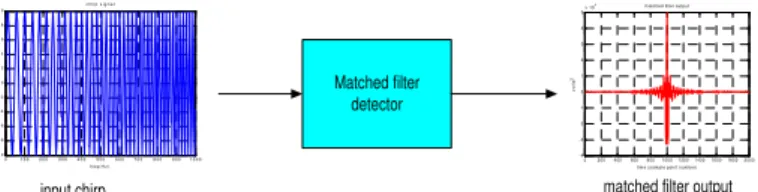
II. MATCHED FILTER DETECTION AT RF The analysis was firstly carried out at RF and this involved generating a simple chirp signal and carrying out the matched filter detection process at RF. The results will then be compared with there corresponding results achieved at QBB so as to come up with a conclusion about investigating the results obtained at QBB. Consider the block diagram below which illustrates the analysis process carried out at RF.

0 1 0 0 2 0 03 0 0 4 0 05 0 0 6 0 07 0 0 8 0 09 0 01 0 0 0 -1 0

-8 -6 -4 -2 0 2 4 6 8 1 0

c h irp s ig n a l

fre q (H z )

vo

lt

s

Matched filter detector

0 200400600800100012001400160018002000 -4

-3 -2 -1 0 1 2 3 4 5

x 104 m at c hed filt er output

t im e (s am ple point num ber)

vo

lt

s2

input chirp matched filter output

Figure 1: RF chirp signal matched filter detection

The input chirp signal is fed into a matched filter whose output is a convolution between the received signal and its time reversed version. Let the chirp input = x , Matlab uses an inbuilt command to execute the time reversal of the chirp input ‘x’

h = fliplr(x) (1) The matched filter then convolves the chirp input ‘x’ with h. The equation below illustrates this.

y=conv(x, h) (2)

Advantages of Matched Filter Detection at

Quadrature Baseband Than at Radio Frequency

Lusungu Ndovi., Member, IAENG

Proceedings of the World Congress on Engineering 2009 Vol I WCE 2009, July 1 - 3, 2009, London, U.K.

(2)

The matched filter output has its peak value at t=T. The theoretical analysis for the QBB simulations is given in the next section and the simulation results which follow in subsequent sections of the chapter will compare the results obtained at RF and QBB.

III. MATHCED FILTER DETECTION AT QBB

The sole purpose of the study is to investigate the possibility of carrying out certain signal processing techniques at quadrature baseband and hence, it is required to outline the theory used to carryout the simulations at QBB. Consider the figure below.

0 1 0 02 0 03 0 04 0 05 0 06 0 07 0 08 0 09 0 01 0 0 0 - 1 0

-8 -6 -4 -2 0 2 4 6 8 1 0 c h irp s ig n a l

fr e q ( H z )

vo

lts

Matched filter detector

at QBB

input chirp

matched filter output X

c

j t

e−ω

LPF Chirp at QBB

0 2 0 04 0 06 0 08 0 01 0 0 01 2 0 01 4 0 01 6 0 01 8 0 02 0 0 0 -1

-0 . 5 0 0 . 5 1 1 . 5 2 2 . 5 3

x 1 04 m a t c h e d fil t e r o u t p u t

t im e (s a m p le p o i n t n u m b e r)

vo

lt

s2

Figure 2: QBB chirp signal matched filter detection

From the figure above, it is seen that the chirp is mixed down and lowpass filtered to quadrature baseband before being fed into the matched filter which has a time-reversed copy of the QBB input chirp. The output does have its peak at t=T as in the previous RF analysis. The simulation results will give a more detailed comparison of the graphical results obtained from the RF and QBB simulations.

| .* j ct|

LPF

xqbb x e−ω

∴ = (3)

The matched filter output should show that a perfect match occurs when the QBB chirp input and its time-reversed copy make a complete overlap at t=T resulting in the large spike at that point.

IV. MATLAB SIMULATION RESULTS

This part of the paper gives the simulation results for the analysis carried out at RF and QBB. The results at RF and QBB are then compared and discussed.

A. RF simulation results

The figures given below show the simulation results obtained for the direct path analysis at RF.

0 100 200 300 400 500 600 700 800 900 1000 -10

-8 -6 -4 -2 0 2 4 6 8 10

chirp signal

freq(Hz)

vo

lt

s

0 100 200 300 400 500 600 700 800 900 1000 0

100 200 300 400 500 600 700 800 900 1000

magnitude spectrum of chirp

m

agn

it

u

de

frequency(Hz)

(b) (a)

0 200 400 600 800 1000 1200 1400 1600 1800 2000 -4

-3 -2 -1 0 1 2 3 4 5x 10

4 _{matched filter output}

time (sample point number)

vo

lt

s

2

(c)

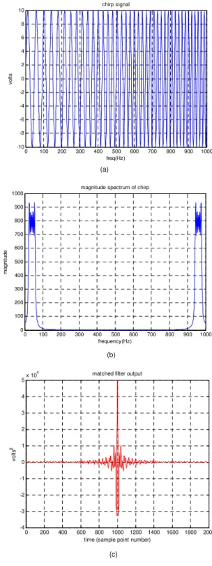
Figure 3: (a) Input chirp (b) Chirp signal magnitude

spectrum (c) Matched filter output.

From the figure as explained under the theoretical analysis, it is seen that the peak of the matched filter output appears at t=T which in the current case due to the discrete domain being used, the point T corresponds to the sample point number n= 1000. The matched filter output has a peak value

(3)

of 5e4 at this point and this value can be verified mathematically. Let y(n) represent the matched filter output in the discrete domain. It should be noted that the convolution is a point-wise multiplication and integration which in the discrete domain is represented by the following operation (2).

1

( )

( ) ( )

N

n

y n

x n h n

=

∑

(4)

Now for the current simulation, the input chirp x was sinusoidal having a peak value of 10 and the sampling frequency ‘fs’=1000. Replacing the expressions for x(n) and

h(n) with the discrete domain versions of x(t) and h(t) and ignoring other parameters of the chirp expect for the amplitude and signal form( i.e. sine or cosine)

we have;

1000

1

( ) ( ) ( )

N

n

y n x n h n

=

∑

(5)

or

1000

1

( ) (10 sin[...])(10 sin[...]) *

N

n

y n =

=

∑

(6)

Note that the * denotes the conjugate of the time-reversed

version of the chirp. It is seen that a product of the two inputs of equation 5 summed from n= 1 to N results in a

trigonometric expression given below which upon applying a trigonometric identity reduces to the equation 7 below.

1 0 0 0 2 1

( ) 1 0 0 sin [....]

n

y n

=

∑

(7) or

1000

1

1 1

( ) 100( cos 2[....]) 2 2

n

y n

=

∑

− (8)

The absolute value of the matched filter output thus reduces to;

4

1 | ( ) |

(1000 100)

5 10

2 y n

=

×

= ×

(9)

Therefore, the output of the matched filter is correct as has been verified numerically.

B. QBB simulation results

The analysis then moves down to quadrature baseband where the matched filter detection is now being implemented at QBB. The figures shown below are the simulation results obtained from the QBB simulation. The parameters of the input chirp are the same as that used for the RF simulation and hence referring to Figure 4 for the input chirp does suffice.

0 100 200 300 400 500 600 700 800 900 1000 0

100 200 300 400 500 600 700 800 900 1000

magnitude spectrum of chirp

m

agni

tud

e

frequency(Hz)

(a)

0 100 200 300 400 500 600 700 800 900 1000 0

100 200 300 400 500 600 700 800 900 1000

magnitude spectrum of down-mixed chirp

m

agni

tud

e

frequency(Hz)

(b)

Figure 4: (a) Chirp signal magnitude spectrum before

down-mixing (b) after down-mixing

(4)

0 100 200 300 400 500 600 700 800 900 1000 0

100 200 300 400 500 600 700 800 900 1000

magnitude spectrum of QBB chirp

m

agn

it

ude

frequency(Hz)

(c)

0 200 400 600 800 1000 1200 1400 1600 1800 2000 -1

-0.5 0 0.5 1 1.5 2 2.5

3x 10

4 _{matched filter output}

time (sample point number)

vo

lt

s

2

(d)

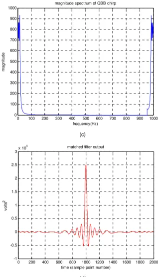
Figure 4: (c) After lowpass filtering down to QBB (d)

Matched filter output.

From the figures above, it is seen that the output of the matched filter at QBB is half the size of the output obtained at RF. This is due to the fact that the down mixing frequency used is equal to the carrier frequency and looking at the spectrum before and after downmixing, it is seen that the spectrum remains symmetrical at QBB and hence the factor of 2 is not required after the lowpass filtering action during the conversion to quadrature baseband and so this reduced the output by a factor of 2. However, it is should be emphasized that this factor does not overshadow the main advantage of working at lower baseband frequencies and it therefore suffices to say that the objective of the direct path analysis has been achieved.

V. CONCLUSION

The analysis carried out does verify the possibility of carrying out matched filter detection at quadrature baseband.

As mentioned earlier, the main advantage of operating at quadrature baseband is that lower frequency of operation is enhanced which also facilitates for lower sampling frequencies.

REFERENCES

[1] http://www.cambridge-en.com, Newsletter 5 -March 1999.html.

[2] Mahafza, Bassem R. “Radar Systems Analysis and

Design Using Matlab” Chapman &Hall/CRC, 2000.