Computational efficient generation of microstructures towards the design of advanced multi-scale heterogeneous materials

Computational efficient generation

of microstructures towards the

design of advanced multi-scale

heterogeneous materials

Professors:

Francisco Manuel Andrade Pires Bernardo Proença Ferreira

Student:

José Luís Passos Vila-Chã

Thesis submitted under the scope of the Master’s degree in Mechanical Engineering

Abstract

Nowadays, the design and modeling of advanced materials calls for the understanding that these are hierarchical in nature, i.e. their macroscopic properties and mechanical response result from the interaction between heterogeneous structures spanning over multiple length scales. Examples of important materials from an industrial standpoint that benefit from this multi-scale approach are polymer blends and composite mate-rials. In this view, the method of computational homogenization emerged as an effec-tive way of modeling multi-scale heterogeneous materials by performing an homoge-nization procedure over a representative volume element (RVE) of the microstructure. However, in order to accurately capture the macroscopic behavior, it is crucial that the RVE contains enough morphological and topological information about the mi-crostructural heterogeneities and is representative in an average sense.

This work presents a computational robust and efficient program in Python, based on a molecular dynamics simulation with a multi-temperature isokinetic scheme, that is able to generate an RVE from a given set of material and geometrical input descrip-tors. In general, these may characterize the material matrix, particles/inclusions, voids and fibers, e.g. radius, ellipsoid axes magnitude and orientation, spatial position, and the corresponding phase in the heterogeneous material, volume fraction and number of particles. The geometrical parameters characterizing the inclusions may be spec-ified by the user as fixed values or be made to vary according to different statistical distributions. Multiple phases are also supported allowing for great flexibility in the modeling of real materials.

The microstructures generated are evaluated using the Minkowski structure met-rics of their Voronoi cells. These are a very versatile tool in the detection of unwanted order or clustering, both undesirable properties in a microstructure whose purpose is to plausibly mimic real matrix-composite materials. Using this technique, the mi-crostructures generated through the proposed approach are validated as it pertains to their "quality".

After the generation procedure, various RVEs are discretized in a suitable finite el-ement mesh in order to perform microscale analyses through computational homog-enization. The various examples considered are created keeping the volume fraction constant and increasing the number of inclusions within the RVE. Submitting the mi-crostructures to various loading conditions and employing different boundary condi-tions, it is concluded that an increase in the number of particles included leads to a more representative volume element. Isotropic responses are also achieved for mi-crostructures containing only Disks and Spheres, as more inclusions are considered.

Resumo

Nos dias de hoje, o projeto e modelação de materiais avançados exige a perceção de que estes são compostos por estruturas hierárquicas, isto é, as suas propriedades macroscópicas e a sua resposta mecânica resultam da interação entre estruturas het-erogéneas que se apresentam a múltiplas escalas. Materiais de grande importância a nível industrial que beneficiam deste tipo de análise a várias escalas são, por exemp-los, as misturas de polímeros e os materiais compósitos. Nesta perspetiva, o método da homogeneização computacional surgiu como uma técnica eficaz de modelar mate-riais heterogéneos a múltiplas escalas, através de um procedimento de homogeneiza-ção ao longo de um elemento de volume representativo (RVE) da microestrutura. To-davia, de modo a capturar com precisão o seu comportamento macroscópico é cru-cial que o RVE contenha um conjunto de informação morfológica e topológica sobre as heterogeneidades à micro escala, sendo representativo do comportamento do ma-terial em média.

Esta tese apresenta um programa computacionalmente robusto e eficiente, escrito em Python, baseado em simulações de dinâmica molecular com esquema isocinético multi temperatura, que é capaz de gerar RVEs a partir de um conjunto de descritores materiais de geométricos de entrada. Em geral, estes podem caraterizar a matriz do material, as sua inclusões, vazios ou fibras, especificando, por exemplo, o raio das partículas, e a fase correspondente, através da sua fração volúmica e numero de in-clusões. Dado que um número arbitrário de fases é permitido, obtém-se uma ferra-menta muito flexível na modelação de materiais reais.

As microestruturas geradas são avaliadas utilizando as métricas estruturais de Min-kowski das suas células Voronoi. Estas são uma ferramenta versátil na deteção de estruturas ordenadas ou aglomerados indesejáveis de partículas, ambas caraterísticas inconvenientes em microestruturas cujo propósito é imitar de forma plausível materi-ais compósitos remateri-ais. Utilizando esta técnica, validaram-se as microestruturas geradas através da abordagem proposta quanto à sua "qualidade".

Depois de gerados, discretizaram-se vários RVEs em malhas de elementos fini-tos apropriadas com o objetivo de levar a cabo análises à micro escala por homo-geneização computacional. Os vários exemplos considerados são criados mantendo a fração volúmica constante, mas aumentando o número de inclusões dentro do RVE. Concluí-se, submetendo as microestruturas a vários esquemas de carregamento me-diante diferentes condições fronteira, que um aumento no número de partículas in-cluídas leva a um volume elementar mais representativo. Verificam-se ainda respostas isotrópicas por parte de microestruturas que contêm apenas Discos e Esferas, à me-dida que mais inclusões são consideradas.

Acknowledgments

I wish to thank both my supervisors, Prof. Francisco Pires and Bernardo Ferreira for their guidance and help during this work. I hope to have fulfilled the goals set forth for this MSc thesis and to have meaningfully contributed to the work developed by the CM2S group.

I am profoundly thankful for all the support and encouragement from my parents and my brother. All my achievements, big and small, in the journey that lead me here can be traced to their unwavering belief in me.

To all the CM2S work group, I wish to express a sincere "thank you" for all the help you provided me.

Contents

Abstract v

Resumo vii

Acknowledgments ix

List of Figures xv

List of Tables xxvii

Notation xxxiii

1 Introduction 1

1.1 Contextualization . . . 1

1.2 Objectives . . . 5

1.3 Computational implementations and numerical simulations . . . 5

1.4 Document structure . . . 5

2 Continuum Mechanics and Finite Element Method 7 2.1 Kinematics of Deformation . . . 7

2.1.1 Motion . . . 7

2.1.2 Material and spatial descriptions . . . 8

2.1.3 Deformation gradient . . . 8

2.2 Strain tensors . . . 10

2.3 Forces and stress measures . . . 11

2.4 Fundamental conservation principles . . . 12

2.5 Weak equilibrium equations . . . 14

2.6 Mechanical constitutive initial value problem . . . 15

2.6.1 Thermodynamics with internal variables . . . 15

2.6.2 Mechanical constitutive initial value problem . . . 17

2.7 Time descretization . . . 20

2.8 Finite Element Method . . . 21

2.8.1 Finite element concept . . . 21

2.8.2 Interpolation functions . . . 21

2.8.3 Interpolation matrix and discrete gradient operators . . . 22

2.8.4 Spatial discretization . . . 23

2.8.5 Newton-Raphson Method . . . 25

2.8.6 Numerical integration . . . 25

3 First-order Homogenization-based Hierarchical Multi-scale Model 27

3.1 The first order homogenized constitutive response . . . 27

3.2 Scale Transition Theory . . . 28

3.2.1 Principle of Scales Separation . . . 28

3.2.2 Multi-scale kinematics . . . 28

3.2.3 Principle of Multi-Scale Virtual Power . . . 30

3.3 Microscale boundary conditions . . . 31

3.3.1 Homogenized stress tensor . . . 33

3.4 Time discretization of the microscale equilibrium problem . . . 34

3.5 Numerical discretization of the microscale equilibrium problem . . . 34

4 Random Heterogeneous Materials 35 4.1 Definition . . . 35

4.2 Impact of the microstructure on the effective properties . . . 36

4.3 Systematic description . . . 37

4.3.1 Preliminaries . . . 37

4.3.2 n-Point Probability Functions . . . . 38

4.3.3 Lineal-Path Function . . . 43

4.3.4 Two-Point Cluster Function . . . 43

4.3.5 Nearest Neighbor Function . . . 44

4.3.6 Voronoi metrics and Minkowski structure metrics . . . 44

4.3.7 n-Particle Probability Densities . . . . 50

4.3.8 Ripley’s K function . . . . 51

5 Computational Microstructure Generation 53 5.1 Microstructure reconstruction from experimental data . . . 53

5.2 Physics based microstructure generation . . . 54

5.3 Geometrical methods . . . 54

5.3.1 Molecular Dynamics . . . 55

5.3.2 Monte Carlo techniques . . . 56

5.3.3 Dense random packing . . . 57

5.4 Randomness . . . 60

5.5 Comparison . . . 62

6 Molecular Dynamics Algorithm 65 6.1 Introduction . . . 65

6.2 Geometrical definition of the particles . . . 66

6.2.1 Disks . . . 66

6.2.2 Ellipses . . . 66

6.2.3 Spheres . . . 67

6.2.4 Ellipsoids . . . 67

6.3 Generation of an initial configuration . . . 68

6.4 Legal configurations . . . 68

6.5 Force computation . . . 69

6.5.1 Periodic boundary conditions . . . 69

6.5.2 Overlap area/volume . . . 69

6.5.3 Speed-up schemes . . . 92

6.6 Integration schemes for the equations of motion . . . 94

6.6.1 Verlet integration scheme . . . 94

Contents xiii

6.7.1 Concept of temperature in molecular dynamics . . . 96

6.7.2 Isokinetic scheme . . . 97

6.7.3 Multi-temperature isokinetic scheme . . . 100

7 Results 109 7.1 Microstructure generation . . . 109

7.1.1 Results regarding the isokinetic scheme . . . 109

7.1.2 Validation of the multi-temperature approach . . . 113

7.1.3 Efficiency . . . 125

7.2 Microstructure Analysis . . . 130

7.2.1 Reconstruction of polygons and detection of s-fold symmetry . . . 130

7.2.2 Quality analysis of microstructures containing Disks of the same size using Minkowski structure metrics . . . 133

7.2.3 Detection of anisotropy in microstructures containing Ellipses us-ing Minkowski structure metrics . . . 151

7.2.4 Reconstruction of polyhedra and detection of s-fold symmetry . . 152

7.2.5 Quality analysis of microstructures containing Spheres of the same size using Minkowski structure metrics . . . 155

7.3 Multi-scale analyses based on computational homogenization . . . 163

7.3.1 One phase containing Disks with same radius . . . 164

7.3.2 Three phases containing Disks with different radii . . . 170

7.3.3 One phase containing Disks and one phase containing Ellipses . . 176

7.3.4 One phase containing Spheres with same radius . . . 183

7.3.5 Three phases containing Spheres with different radii . . . 189

7.3.6 One phase containing Spheres and one phase containing Ellipsoids 195 8 Conclusions and Future Research 203 8.1 Conclusions . . . 203

8.2 Future Research . . . 205

List of Figures

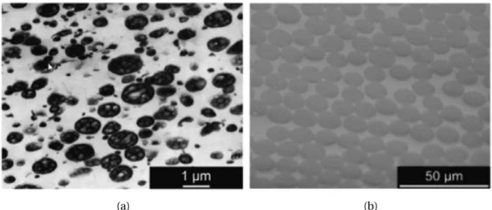
1.1 (a): Polymer blend ABS with ellipsoidal shape inclusions. (b): Fiber-reinforced composite with cylindrical shape inclusions (Adapted from Bargmann et al. (2018)). . . 2 1.2 Pure gas porosity in die casting. The high concentration of gas bubbles

probably caused by too much lubricant or from water leaking into the die. (Adapted from (Walkington and Association, 2003)). . . 3 2.1 Motion . . . 8 2.2 Quasi-static mechanical constitutive initial boundary value problem. . . 18 4.1 A portion of a realizationω of a two-phase random medium, where phase

1 is the white region

_V

V

4.2 Two examples of statistically inhomogeneous media. (a): Density of the gray phase decreases radially from the center.(b): Density of the gray phase decreseas in the upward direction. . . 40 4.3 Two examples of portions of statistically homogeneous media with two

phase. (a): The layered medium is statistically anisotropic. (b): The medium is statistically isotropic. . . 41 4.4 Voronoi diagrams of 100 points obtained through a Poisson point

pro-cess. (a): 2D and (b): 3D. . . 44 4.5 2D set Voronoi diagrams for (a) disks with different radii, (b) ellipses. . . 45 4.6 3D set Voronoi diagrams for (a) spheres with different radii and (b)

ellip-soids. . . 46 4.7 Convex polygon K with sides Lk and corresponding outer normals nk,

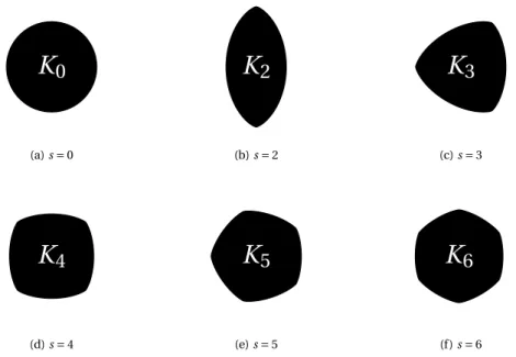
k = 0,...,6. . . . 47 4.8 Shapes containing s-fold, but not higher, symmetry, obtained from the

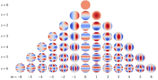
density functionρKs(ϕ) = 1 + cos(sϕ), s = 0, 2, 3,4, 5, 6, 0 ≤ ϕ < 2π. . . 48 4.9 Spherical harmonics Y_sm(n), s = 0, 1, 2, 3, 4, 5, 6, −s ≤ m ≤ s, with n ∈

S2, where S2is the unit sphere. Red represents positive values and blue negative values. . . 49 4.10 Shapes containing s-fold, but not higher, symmetry, obtained from the

density functionρKs,m(n) = 1 + Y

m

s (n), s = 0, 2, 3,4, 5, 6 and −s ≤ m ≤ s,

with n ∈ S2, where S2is the unit sphere. Red marks points with higher curvature and blue points with lower curvature. . . 50 6.1 Diagram containing the parameters defining geometrically the particles

admissible in the microstructures: (a) Disk, (b) Ellipse, (c) Sphere and (d) Ellipsoid. . . 68

6.2 Diagram depicting the approach taken to compute the overlap area be-tween two disk of different radii. . . 70 6.3 Different types of circular segments: (a) less than_{π radians and (b) more}

thanπ radians. . . 71 6.4 Diagram of the standard parametric representation of an ellipse using

inscribed and circumscribed circles. . . 72 6.5 Different types of ellipse segments: (a) less thanπ radians and (b) more

thanπ radians. . . 73 6.6 Absolute coordinate system an coordinate systems corresponding to

El-lipse 1 and ElEl-lipse 2. . . 74 6.7 Possible cases for the intersection of two ellipses, when the number of

intersection points is 0: (a) Ellipse 2 is entirely inside Ellipse 1 and (b) the two Ellipses do not intersect. . . 77 6.8 Possible cases for the intersection of two ellipses, when the number of

intersection points is 1: (a) Ellipse 2 is entirely inside Ellipse 1 and (b) the two Ellipses do not intersect. . . 78 6.9 Possible cases for the intersection of two ellipses, when the number of

intersection points is 2. . . 78 6.10 Possible cases for the intersection of two ellipses, when the number of

intersection points is 3, (a), or 4, (b). . . 79 6.11 Diagram depicting the approach taken to compute the overlap volume

between two Spheres of different radii. . . 82 6.12 Monte Carlo integration of the overlap between two Ellipsoids. The

over-lap volume is the product of the volume of the Ellipsoid where the ran-dom points are generated and the fraction of ranran-dom points inside both Ellipsoids. . . 90 6.13 Diagram illustrating the cell list method. The Disks with radius r whose

center is in the cell i (dark gray) interact only with particles whose center is in the cell i or in the neighboring cells (light gray). . . . 92 6.14 Diagram illustrating the Verlet list method: (a) The Verlet list is

calcu-lated. (b) Disk i interacts only with the Disks whose neighborhood inter-sect its own. (c) Disk i exited its neighborhood, so a new Verlet list must be computed. . . 94 6.15 Diagram for the prediction related to the behavior of a system of

parti-cles applying the isokinetic scheme, as it relates to the elimination of the initial overlap area and the mean overlap area at different temperatures. 99 6.16 Two disks colliding at a velocity kvrefk corresponding to the mean

veloc-ity at temperature Tref. . . 99

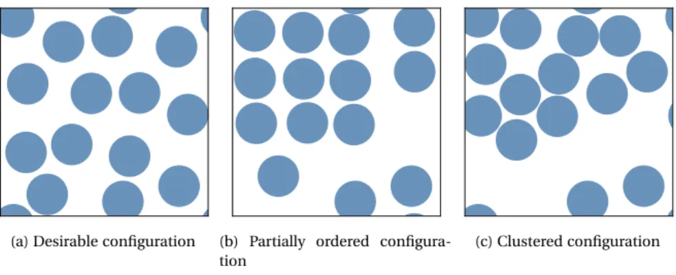
6.17 Examples of desirable and undesirable, both clustered and partially or-dered, configurations. . . 101 6.18 Diagram of the evolution of the total overlap area AOverlapusing the

pro-posed multi-temperature isokinetic scheme. The system spends teq1 and

teq2 at temperatures T1 and T2, achieving the mean overlap area ¯AT1

and ¯AT2, respectively. After reaching the maximum total overlap allowed,

AMax, the simulation is still run for more trelaxand then terminated. . . . 102

6.19 Initial configuration generated through a Poisson point process for a sys-tem of Disks with the same radius. . . 103 6.20 Two particles overlapping at the moment of maximum overlap with the

List of Figures xvii

6.21 Force between two disks and two spheres, where kfk is the area/volume overlap and m is the total area/volume, as a function of the distance be-tween them d /r , where d is the distance bebe-tween the centers and r is the radius of the Spheres/Disks. . . 105 7.1 Total overlap area for a system of 100 Disks with the volume fraction of

0.65 at different reference temperatures given by Trefkb= 2.5 × 10−5/

p 2−k with k = 5, 0, -5, -10, -15, -20, -25, -30 as a function of the number of iterations. . . 110 7.2 Total overlap volume for a system of 50 Spheres with the volume fraction

of 0.3 at different reference temperatures given by Trefkb= 2.5 × 10−5/

p 2−k with k = 5, 0, -5, -10, -15, -20, -25, -30 as a function of the number of it-erations. . . 110 7.3 Total overlap area for a system of 100 Disks at temperature Trefkb= 2.5 × 10−5

with different volume fractions as a function of the number of iterations. 111 7.4 Total overlap volume for a system of 50 Spheres at temperature Trefkb=

2.5 × 10−5with different volume fractions, as a function of the number of iterations. . . 111 7.5 Total overlap area for systems of Disks with a volume fraction of 0.65 at

temperature Trefkb= 2.5 × 10−5and a different number of particles as a

function of the number of iterations. . . 112 7.6 Total overlap volume for systems of Spheres with a volume fraction of 0.3

at temperature Trefkb= 2.5 × 10−5and a different number of particles as

a function of the number of iterations. . . 112 7.7 Total overlap area for a system of 100 Disks with volume fraction equal to

0.65 as function of the number of iterations, allowing a different number of iterations, k, for the equilibration time in the multi-temperature isoki-netic scheme. A configuration is accepted as legal if there are no overlaps. 115 7.8 Final microstructures containing 100 Disks with a volume fraction equal

to 0.65, allowing a different number of iterations, k, for the equilibration time in the multi-temperature isokinetic scheme. A configuration is ac-cepted as legal if there are no overlaps. . . 115 7.9 Total overlap area for four different random samples of a system

con-taining 100 Disks with volume fraction equal to 0.65 as a function of the number of iterations, allowing 25 iterations for the equilibration time in the multi-temperature isokinetic scheme. A configuration is accepted as legal if there are no overlaps. . . 116 7.10 Final microstructures corresponding to four different random samples of

a system containing 100 Disks with a volume fraction equal to 0.65, al-lowing 25 iterations for the equilibration time in the multi-temperature isokinetic scheme. A configuration is accepted as legal if there are no overlaps. . . 116 7.11 Total overlap area for systems containing a different numbers of Disks,

n = 10, 15, 30, 50, 100 and 200, with volume fraction equal to 0.65 as a

function of the number of iterations, allowing 25 iterations for the equili-bration time in the multi-temperature isokinetic scheme. A configuration is accepted as legal if there are no overlaps. . . 117

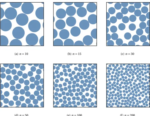
7.12 Final microstructures for systems containing a different numbers of Disks,

n = 10, 15, 30, 50, 100 and 200, with volume fraction equal to 0.65

al-lowing 25 iterations for the equilibration time in the multi-temperature isokinetic scheme. A configuration is accepted as legal if there are no overlaps. . . 117 7.13 Total overlap area for systems containing 100 Disks, with different

vol-ume fractions, vf = 0.1, 0.25, 0.50, 0.65, 0.80 and 0.9, as a function of the number of iterations, allowing 25 iterations for the equilibration time in the multi-temperature isokinetic scheme. A configuration is accepted as legal if there are no overlaps. . . 118 7.14 Final microstructures for systems containing 100 Disks, with different

volume fractions, vf = 0.1, 0.25, 0.50, 0.65, 0.80 and 0.9, allowing 25 it-erations for the equilibration time in the multi-temperature isokinetic scheme. A configuration is accepted as legal if there are no overlaps. . . . 118 7.15 Total overlap area for systems containing a different numbers of Disks,

n = 10, 15, 30, 50, 100 and 200, with volume fraction equal to 0.65 as a

function of the number of iterations, "self-calibrating" the equilibration time in the multi-temperature isokinetic scheme. A configuration is ac-cepted as legal if there are no overlaps. . . 119 7.16 Final microstructures for systems containing a different numbers of Disks,

n = 10, 15, 30, 50, 100 and 200, with volume fraction equal to 0.65,

"self-calibrating" the equilibration time in the multi-temperature isokinetic scheme. A configuration is accepted as legal if there are no overlaps. . . . 119 7.17 Total overlap area for systems containing 100 Disks, with different

vol-ume fractions, vf = 0.7, 0.75, 0.80, 0.85 and 0.9, as a function of the num-ber of iterations, "self-calibrating" the equilibration time in the multi-temperature isokinetic scheme. A configuration is accepted as legal if there are no overlaps. . . 120 7.18 Final microstructures for systems containing 100 Disks, with different

volume fractions, vf = 0.7, 0.75, 0.80, 0.85 and 0.9, as a function of the number of iterations, "self-calibrating" the equilibration time in the multi-temperature isokinetic scheme. A configuration is accepted as legal if there are no overlaps. . . 120 7.19 Total overlap area for systems containing a different numbers of Spheres,

n = 10, 15, 30, 50, 100 and 200, with volume fraction equal to 0.3 as a

function of the number of iterations, "self-calibrating" the equilibration time in the multi-temperature isokinetic scheme. A configuration is ac-cepted as legal if the total overlap volume is smaller than 1 × 10−10. . . 121 7.20 Final microstructures for systems containing a different numbers of Spheres,

n = 10, 15, 30, 50, 100 and 200, with volume fraction equal to 0.3 as a

function of the number of iterations, "self-calibrating" the equilibration time in the multi-temperature isokinetic scheme. A configuration is ac-cepted as legal if the total overlap volume is smaller than 1 × 10−10. . . 121 7.21 Total overlap area for systems containing 100 Spheres, with different

vol-ume fractions, vf = 0.1, 0.2, 0.3, 0.4, 0.5 and 0.6, as a function of the num-ber of iterations, "self-calibrating" the equilibration time in the multi-temperature isokinetic scheme. A configuration is accepted as legal if the total overlap volume is smaller than 1 × 10−10_{. . . 122}

List of Figures xix

7.22 Final microstructures for systems containing 100 Spheres, with differ-ent volume fractions, vf = 0.1, 0.2, 0.3, 0.4, 0.5 and 0.6, as a function of the number of iterations, "self-calibrating" the equilibration time in the multi-temperature isokinetic scheme. A configuration is accepted as le-gal if the total overlap volume is smaller than 1 × 10−10. . . 122 7.23 Total overlap area for systems containing 20 Ellipses with different ratios

between the principal axis, a/b = 1, 1.5, 2, 2.5 and 3, at volume fraction of 0.5, as a function of the number of iterations, "self-calibrating" the equilibration time in the multi-temperature isokinetic scheme. A config-uration is accepted as legal if there are no overlaps. . . 123 7.24 Total overlap area for systems containing 20 Ellipses with different ratios

between the principal axis, a/b = 1, 1.5, 2, 2.5 and 3, at volume fraction of 0.5, as a function of the number of iterations, "self-calibrating" the equilibration time in the multi-temperature isokinetic scheme. A config-uration is accepted as legal if there are no overlaps. . . 123 7.25 (a) Average CPU time and (b) average number of iterations averaged over

five samples, for the generation of microstructures containing different numbers of Disks, n = 5, 10, 20, 50 , 100, 200 and 500, at various volume fractions, vf = 0.1, 0.2, 0.3, 0.4, 0.5, 0.6 and 0.7, using the "self-calibrating" multi-temperature isokinetic scheme. A configuration is accepted as le-gal if there are no overlaps. . . 126 7.26 (a) Average CPU time and (b) average number of iterations averaged over

five samples, for the generation of microstructures containing different numbers of Spheres, n = 10, 20, 50, 100, 200 and 500, at various volume fractions, vf = 0.1, 0.2, 0.3, 0.4, and 0.5, using the "self-calibrating" multi-temperature isokinetic scheme. A configuration is accepted as legal if the average total overlap area per particle is smaller than 1 × 10−12. . . 127 7.27 (a) Average CPU time and (b) average number of iterations averaged over

five samples, for the generation of microstructures containing 20 Ellipses at a volume fraction of 0.5, with different ratios between the principal axis, a/b = 1, 1.5, 2, 2.5 and 3, using the "self-calibrating" multi-temperature isokinetic scheme. A configuration is accepted as legal if there are no overlaps. . . 128 7.28 (a): Convex polygon obtained distorting and adding vertices to an

equi-lateral triangle. (b): Reconstruction using the first 6 terms of the Fourier series to approximate the polygon’s curvature (c): Minkowski structure metrics of the polygon. . . 130 7.29 (a): Non-convex polygon obtained distorting and adding vertices to an

equilateral triangle. (b): Minkowski structure metrics of the polygon. . . . 131 7.30 (a): Convex polygon obtained distorting and adding vertices to a square.

(b): Reconstruction using the first 6 terms of the Fourier series to ap-proximate the polygon’s curvature. (c): Minkowski structure metrics of the polygon. . . 131 7.31 (a): Non-convex polygon obtained distorting and adding vertices to a

square. (b): Minkowski structure metrics of the polygon. . . 131 7.32 (a): Convex polygon obtained distorting and adding vertices to a thin

rectangle. (b): Reconstruction using the first 6 terms of the Fourier series to approximate the polygon’s curvature (c): Minkowski structure metrics of the polygon. . . 131

7.33 (a): Non-convex polygon obtained distorting and adding vertices to a thin rectangle. (b): Minkowski structure metrics of the polygon. . . 132 7.34 (a): Convex polygon obtained distorting and adding vertices to an

equi-lateral triangle. (b): Reconstruction using the first 6 terms of the Fourier series to approximate the polygon’s curvature (c): Minkowski structure metrics of the polygon. . . 132 7.35 (a): Non-convex polygon obtained distorting and adding vertices to a

regular hexagon. (b): Minkowski structure metrics of the polygon. . . 132 7.36 (a) Voronoi diagram of a microstructure containing 50 Disks at a volume

fraction equal to 0.5, with the cells colored according to their perimeter. (b) Histogram containing the perimeter of the Voronoi cells. . . 134 7.37 (a) Voronoi diagram of a microstructure containing 50 Disks at a

vol-ume fraction equal to 0.5, with the cells colored according to their q2

Minkowski structure metric. (b) Histogram containing the q2Minkowski

structure metric of the Voronoi cells, where the dashed line represents the average. . . 134 7.38 (a) Voronoi diagram of a microstructure containing 50 Disks at a

vol-ume fraction equal to 0.5, with the cells colored according to their q3

Minkowski structure metric. (b) Histogram containing the q3Minkowski

structure metric of the Voronoi cells, where the dashed line represents the average. . . 135 7.39 (a) Voronoi diagram of a microstructure containing 50 Disks at a

vol-ume fraction equal to 0.5, with the cells colored according to their q4

Minkowski structure metric. (b) Histogram containing the q4Minkowski

structure metric of the Voronoi cells, where the dashed line represents the average. . . 135 7.40 (a) Voronoi diagram of a microstructure containing 50 Disks at a

vol-ume fraction equal to 0.5, with the cells colored according to their q5

Minkowski structure metric. (b) Histogram containing the q5Minkowski

structure metric of the Voronoi cells, where the dashed line represents the average. . . 136 7.41 (a) Voronoi diagram of a microstructure containing 50 Disks at a

vol-ume fraction equal to 0.5, with the cells colored according to their q6

Minkowski structure metric. (b) Histogram containing the q6Minkowski

structure metric of the Voronoi cells, where the dashed line represents the average. . . 136 7.42 Microstructures containing excessive order, signaled by the

concentra-tion of cells with high q2, (a), q3, (b), q4, (c) and q6, (d) Minkowski

struc-ture metrics. . . 137 7.43 Histograms of the perimeter and Minkowski structure metrics, q2, q3, q4,

q5 and q6, for five random samples containing 100 Disks at a volume

fraction of 0.3. . . 138 7.44 Histograms of the perimeter and Minkowski structure metrics, q2, q3, q4,

q5 and q6, for five random samples containing 100 Disks at a volume

fraction of 0.5. . . 139 7.45 Histograms of the perimeter and Minkowski structure metrics, q2, q3, q4,

q5 and q6, for five random samples containing 100 Disks at a volume

List of Figures xxi

7.46 Final microstructures for random samples generated with the "self-calibrating" multi-temperature isokinetic scheme (Method 1) and three samples gen-erated using the multi-temperature isokinetic scheme with a low fixed number of equilibration iterations (Method 2), all containing 100 Disks at a volume fractions of 0.3, 0.5 and 0.7. . . 142 7.47 Histograms of the perimeter and Minkowski structure metrics, q2, q3, q4,

q5and q6, for three random samples generated with the "self-calibrating"

multi-temperature isokinetic scheme (Method 1) and three samples gen-erated using the multi-temperature isokinetic scheme with a low fixed number of equilibration iterations (Method 2), all containing 100 Disks at a volume fraction of 0.3. . . 143 7.48 Histograms of the perimeter and Minkowski structure metrics, q2, q3, q4,

q5and q6, for three random samples generated with the "self-calibrating"

multi-temperature isokinetic scheme (Method 1) and three samples gen-erated using the multi-temperature isokinetic scheme with a low fixed number of equilibration iterations (Method 2), all containing 100 Disks at a volume fraction of 0.5. . . 144 7.49 Histograms of the perimeter and Minkowski structure metrics, q2, q3, q4,

q5and q6, for three random samples generated with the "self-calibrating"

multi-temperature isokinetic scheme (Method 1) and three samples gen-erated using the multi-temperature isokinetic scheme with a low fixed number of equilibration iterations (Method 2), all containing 100 Disks at a volume fraction of 0.7. . . 145 7.50 Boxplots of the mean, standard deviation, skewness and kurtosis of the

perimeter, P , and Minkowski structure metrics, q2, q3, q4, q5 and q6

of the Voronoi cells, for five random samples generated with the "self-calibrating" multi-temperature isokinetic scheme (Method 1) and three samples generated using the multi-temperature isokinetic scheme with a low fixed number of equilibration iterations (Method 2), all containing 100 Disks at a volume fraction of 0.3. . . 146 7.51 Boxplots of the mean, standard deviation, skewness and kurtosis of the

perimeter, P , and Minkowski structure metrics, q2, q3, q4, q5 and q6

of the Voronoi cells, for five random samples generated with the "self-calibrating" multi-temperature isokinetic scheme (Method 1) and three samples generated using the multi-temperature isokinetic scheme with a low fixed number of equilibration iterations (Method 2), all containing 100 Disks at a volume fraction of 0.5. . . 147 7.52 Boxplots of the mean, standard deviation, skewness and kurtosis of the

perimeter, P , and Minkowski structure metrics, q2, q3, q4, q5 and q6

of the Voronoi cells, for five random samples generated with the "self-calibrating" multi-temperature isokinetic scheme (Method 1) and three samples generated using the multi-temperature isokinetic scheme with a low fixed number of equilibration iterations (Method 2), all containing 100 Disks at a volume fraction of 0.7. . . 148

7.53 (a): Set Voronoi diagram for a microstructure containing 30 Ellipses with ratio a/b equal to 2.5 oriented alongπ/4 at a volume fraction of 0.6, with the Voronoi cells colored according to their Minkowski structure metric

q2. (b): Voronoi diagram for a microstructure containing 30 Disks at a

volume fraction of 0.6, with the Voronoi cells colored according to their Minkowski structure metric q2. (c): Histogram of the Minkowski

struc-ture metric q2of both microstructures. (d) Histogram of the argument of

the irreducible Minkowski tensorψ2of both microstructures. . . 152

7.54 (a): Hexagonal prism. (b): Reconstruction found approximating the cur-vature through a series of spherical harmonics, where points in red rep-resent high curvature and points in blue low curvature. (c) Minkowski structure metrics of the hexagonal prism. . . 153 7.55 (a): Tetrahedron. (b): Reconstruction found approximating the curvature

through a series of spherical harmonics, where points in red represent high curvature and points in blue low curvature. (c) Minkowski structure metrics of the tetrahedron. . . 153 7.56 (a): Cube. (b): Reconstruction found approximating the curvature through

a series of spherical harmonics, where points in red represent high cur-vature and points in blue low curcur-vature. (c) Minkowski structure metrics of the cube. . . 154 7.57 (a): Thin parallelepiped. (b): Reconstruction found approximating the

curvature through a series of spherical harmonics, where points in red represent high curvature and points in blue low curvature. (c) Minkowski structure metrics of the thin parallelepiped. . . 154 7.58 (a) Voronoi diagram of a microstructure containing 100 Spheres at a

vol-ume fraction equal to 0.4, with the cells colored according to their surface area. (b) Histogram containing the surface area of the Voronoi cells. . . . 155 7.59 (a) Voronoi diagram of a microstructure containing 100 Spheres at a

vol-ume fraction equal to 0.4, with the cells colored according to their q2

Minkowski metric. (b) Histogram containing the q2Minkowski metric of

the Voronoi cells, where the dashed line represents the average. . . 156 7.60 (a) Voronoi diagram of a microstructure containing 100 Spheres at a

vol-ume fraction equal to 0.4, with the cells colored according to their q3

Minkowski metric. (b) Histogram containing the q3Minkowski metric of

the Voronoi cells, where the dashed line represents the average. . . 156 7.61 (a) Voronoi diagram of a microstructure containing 100 Spheres at a

vol-ume fraction equal to 0.4, with the cells colored according to their q4

Minkowski metric. (b) Histogram containing the q4Minkowski metric of

the Voronoi cells, where the dashed line represents the average. . . 157 7.62 (a) Voronoi diagram of a microstructure containing 100 Spheres at a

vol-ume fraction equal to 0.4, with the cells colored according to their q5

Minkowski metric. (b) Histogram containing the q5Minkowski metric of

the Voronoi cells, where the dashed line represents the average. . . 157 7.63 (a) Voronoi diagram of a microstructure containing 100 Spheres at a

vol-ume fraction equal to 0.4, with the cells colored according to their q6

Minkowski metric. (b) Histogram containing the q6Minkowski metric of

List of Figures xxiii

7.64 (a): Voronoi diagram of a microstructure containing Spheres arranged in a cubic grid with random vertices missing. Only the cells with Minkowski structure metric q4higher than 0.7 are shown. (b): Voronoi diagram of a

microstructure containing Spheres at a volume fraction of 0.7. Only the cells with Minkowski structure metric q6higher than are 0.5 shown. . . . 158

7.65 Histograms of the surface area and Minkowski structure metrics, q2, q3,

q4, q5and q6, for five random samples containing 100 Spheres at a

vol-ume fraction of 0.1. . . 159 7.66 Histograms of the surface area and Minkowski structure metrics, q2, q3,

q4, q5and q6, for five random samples containing 100 Spheres at a

vol-ume fraction of 0.3. . . 160 7.67 Histograms of the surface area and Minkowski structure metrics, q2, q3,

q4, q5and q6, for five random samples containing 100 Spheres at a

vol-ume fraction of 0.5. . . 161 7.68 Microstructures containing (a): 3, (b): 32, (c):178 and (d):1000 Disks of

the same size belonging to the same phase at a volume fraction equal to 0.3. The TRI6 nonconform mesh is only represented for (a) and (b) (only the vertex nodes shown). . . 165 7.69 Homogenized first Piola-Kirchhoff stress for various loading schemes ((a):

uniaxial traction along xx - Pxx, (b): uniaxial traction along y y - Py y, (c):

simple shear across x y - Px y) as a function of the number of particles,

for microstructures containing only Disks of the same size at a volume fraction equal to 0.3 belonging to the same phase. . . 166 7.70 Microstructures containing (a): 3, (b): 32, (c):178 and (d):1000 Disks of

the same size belonging to the three different phases (Phase 2: vf = 0.1, Phase 3: vf = 0.05, Phase 4: vf = 0.15). The TRI6 nonconform mesh is only represented for (a) and (b) (only the vertex nodes shown). . . 171 7.71 Homogenized first Piola-Kirchhoff stress for various loading schemes ((a):

uniaxial traction along xx - Pxx, (b): uniaxial traction along y y - Py y, (c):

simple shear across x y - Px y) as a function of the number of particles, for

microstructures containing Disks of the same size belonging to the three different phases (Phase 2: vf = 0.1, Phase 3: vf = 0.05, Phase 4: vf = 0.15). . 172 7.72 Microstructures containing (a): 4, (b): 32, (c):178 and (d):1000 particles

including two particle phases, Phase 2 containing Disks of the same size at vf = 0.1 and Phase 3 containing Ellipses oriented along xx at vf = 0.2. The TRI6 nonconform mesh is only represented for (a) and (b) (only the vertex nodes shown). . . 177 7.73 Homogenized first Piola-Kirchhoff stress for various loading schemes ((a):

uniaxial traction along xx - Pxx, (b): uniaxial traction along y y - Py y, (c):

simple shear across x y - Px y) as a function of the number of particles, for

microstructures containing two particle phases, Phase 2 containing Disks of the same size at vf = 0.1 and Phase 3 containing Ellipses oriented along

7.74 Relative variation of the homogenized first Piola-Kirchhoff Pxxunder

uni-axial loading along xx between the linear and uniform traction bound-ary conditions and the periodic boundbound-ary condition as a function of the number of particles. Microstructure 1 includes one particle phase con-taining Disks of the same size at a volume fraction equal to 0.3. Mi-crostructure 2 includes three particle phases containing Disks of the same size, Phase 2 at a volume fraction of 0.1, Phase 3 at a volume fraction of 0.05 and Phase 4 at a volume fraction 0.15. Microstructure 3 comprises two particle phase. Phase 2 containing Disks of the same size at a volume fraction equal to 0.1 and Phase 3 containing Ellipses at a volume fraction equal to 0.2 oriented along xx. . . 181 7.75 Microstructures containing (a): 3, (b): 32, (c):178 and (d):562 Spheres of

the same size belonging to the same phase at a volume fraction equal to 0.2. The TETRA10 nonconform mesh is only represented for (a) and (b) (only the vertex nodes shown). . . 184 7.76 Homogenized first Piola-Kirchhoff stress for various loading schemes ((a):

uniaxial traction along xx - Pxx, (b): uniaxial traction along y y - Py y, (c):

uniaxial traction along zz - Pzz, (d): simple shear across x y - Px y) as a

function of the number of particles, for microstructures containing only Spheres of the same size at a volume fraction equal to 0.2 belonging to the same phase. . . 185 7.77 Microstructures containing (a): 3, (b): 32, (c):178 and (d):562 Spheres of

the same size belonging to three different phases (Phase 2: vf = 0.075, Phase 3: vf = 0.025, Phase 4: vf = 0.1). The TETRA10 nonconform mesh is only represented for (a) and (b) (only the vertex nodes shown). . . 190 7.78 Homogenized first Piola-Kirchhoff stress for various loading schemes ((a):

uniaxial traction along xx - Pxx, (b): uniaxial traction along y y - Py y,

(c): uniaxial traction along zz - Pzz, (d): simple shear across x y - Px y)

as a function of the number of particles, for microstructures containing Spheres of the same size belonging to three different phases (Phase 2: vf = 0.075, Phase 3: vf = 0.025, Phase 4: vf = 0.1). . . 191 7.79 Microstructures containing (a): 4, (b): 32, (c):178 and (d):562 particles

including two particle phases, Phase 2 containing Spheres of the same size at vf = 0.1 and Phase 3 containing Ellipsoids with the largest princi-pal axis oriented along xx at vf = 0.1. The TETRA10 nonconform mesh is only represented for (a) and (b) (only the vertex nodes shown). . . 196 7.80 Homogenized first Piola-Kirchhoff stress for various loading schemes ((a):

uniaxial traction along xx - Pxx, (b): uniaxial traction along y y - Py y, (c):

uniaxial traction along zz - Pzz, (d): simple shear across x y - Px y) as a

function of the number of particles, for microstructures including two particle phases, Phase 2 containing Spheres of the same size at vf = 0.1 and Phase 3 containing Ellipsoids with the largest principal axis oriented along xx at vf = 0.1. . . 197

List of Figures xxv

7.81 Relative variation of the homogenized first Piola-Kirchhoff Pxxunder

uni-axial loading along xx between the linear and uniform traction bound-ary conditions, with reference to the latter, as a function of the num-ber of particles. Microstructure 1 includes one particle phase containing Spheres of the same size at a volume fraction equal to 0.2. Microstruc-ture 2 includes three particle phases containing Spheres of the same size, Phase 2 at a volume fraction of 0.075, Phase 3 at a volume fraction of 0.025 and Phase 4 at a volume fraction 0.1. Microstructure 3 comprises two particle phase. Phase 2 containing Spheres of the same size at a vol-ume fraction equal to 0.1 and Phase 3 containing Ellipsoids at a volvol-ume fraction equal to 0.1 oriented along xx. . . 200

List of Tables

6.1 Correspondence between the values of the coefficients ηi, i = 1,...,5,

found from the coefficients of the characteristic equation of the two El-lipsoid, pk, k = 1,...5, and the relative configuration of the two Ellipsoids. 86

7.1 Average CPU time and corresponding standard deviation from five sam-ples, for the generation of microstructures containing different numbers of Disks, n = 5, 10, 20, 50 , 100, 200 and 500, at various volume fractions, vf = 0.1, 0.2, 0.3, 0.4, 0.5, 0.6 and 0.7, using the "self-calibrating" multi-temperature isokinetic scheme. A configuration is accepted as legal if there are no overlaps. . . 126 7.2 Average CPU time and corresponding standard deviation from five

sam-ples, for the generation of microstructures containing different numbers of Spheres, n = 10, 20, 50, 100, 200 and 500, at various volume frac-tions, vf = 0.1, 0.2, 0.3, 0.4, and 0.5, using the "self-calibrating" multi-temperature isokinetic scheme.A configuration is accepted as legal if the average total overlap area per particle is smaller than 1 × 10−12_{. . . 127}

7.3 Average CPU time, corresponding standard deviation and average final overlap volume and corresponding standard deviation for systems con-taining 10, 20, 50, 100, 200 and 500 Spheres at a volume fraction of 0.6. . 128 7.4 Average CPU time and corresponding standard deviation from five

sam-ples, for the generation of microstructures containing 20 Ellipses at a volume fraction of 0.5, with different ratios between the principal axis,

a/b = 1, 1.5, 2, 2.5 and 3, using the "self-calibrating" multi-temperature

isokinetic scheme. A configuration is accepted as legal if there are no overlaps. . . 128 7.5 Anderson-Darling test probing if the perimeter and Minkowski structure

metrics, q2, q3, q4, q5and q6of the Voronoi cells of five samples all

con-taining 50, 100, 200 or 500 Disks at volume fractions equal to 0.2, 0.3, 0.4, 0.5, 0.6 or 0.7 come from the same underlying distribution. The test is also perform including all the microstructures containing different num-bers of particles with the same volume fraction under "All". The p-value is floored at 25% and capped at 0.1%. . . 141 7.6 Homogenized first Piola-Kirchhoff component Pxx under uniaxial

load-ing condition along xx for linear, periodic, and uniform traction bound-ary conditions as a function of the number of particles, for microstruc-tures containing only Disks of the same size at a volume fraction equal to 0.3 belonging to the same phase. The relative variation with reference to the periodic boundary is also presented asεPeriodic. . . 167

7.7 Homogenized first Piola-Kirchhoff component Py y under uniaxial

load-ing condition along y y for linear, periodic, and uniform traction bound-ary conditions as a function of the number of particles, for microstruc-tures containing only Disks of the same size at a volume fraction equal to 0.3 belonging to the same phase. The relative variation with reference to the periodic boundary is also presented as_εPeriodic. . . 167

7.8 Homogenized first Piola-Kirchhoff component Px y under simple shear

across x y for linear, periodic, and uniform traction boundary conditions as a function of the number of particles, for microstructures containing only Disks of the same size at a volume fraction equal to 0.3 belonging to the same phase. The relative variation with reference to the periodic boundary is also presented as_εPeriodic. . . 168

7.9 Homogenized first Piola-Kirchhoff component Pxxand Py y under

uniax-ial loading condition along xx and y y, respectively, for periodic bound-ary conditions as a function of the number of particles, for microstruc-tures containing only Disks of the same size at a volume fraction equal to 0.3 belonging to the same phase. The relative variation with reference to the homogenized first Piola-Kirchhoff component Pxxunder uniaxial

loading condition along xx is also presented asεxx. . . 168

7.10 Homogenized first Piola-Kirchhoff component Pxx under uniaxial

load-ing condition along xx for linear, periodic, and uniform traction bound-ary conditions as a function of the number of particles, for microstruc-tures containing Disks of the same size belonging to the three different phases (Phase 2: vf = 0.1, Phase 3: vf = 0.05, Phase 4: vf = 0.15). The rel-ative variation with reference to the periodic boundary is also presented asεPeriodic. . . 173

7.11 Homogenized first Piola-Kirchhoff component Py y under uniaxial

load-ing condition along y y for linear, periodic, and uniform traction bound-ary conditions as a function of the number of particles, for microstruc-tures containing Disks of the same size belonging to the three different phases (Phase 2: vf = 0.1, Phase 3: vf = 0.05, Phase 4: vf = 0.15). The rel-ative variation with reference to the periodic boundary is also presented asεPeriodic. . . 173

7.12 Homogenized first Piola-Kirchhoff component Px y under simple shear

across x y for linear, periodic, and uniform traction boundary conditions as a function of the number of particles, for microstructures containing Disks of the same size belonging to the three different phases (Phase 2: vf = 0.1, Phase 3: vf = 0.05, Phase 4: vf = 0.15). The relative variation with reference to the periodic boundary is also presented asεPeriodic. . . 174

7.13 Homogenized first Piola-Kirchhoff component Pxxand Py y under

uniax-ial loading condition along xx and y y, respectively, for periodic bound-ary conditions as a function of the number of particles, for microstruc-tures containing Disks of the same size belonging to the three different phases (Phase 2: vf = 0.1, Phase 3: vf = 0.05, Phase 4: vf = 0.15). The relative variation with reference to the homogenized first Piola-Kirchhoff component Pxx under uniaxial loading condition along xx is also

List of Tables xxix

7.14 Homogenized first Piola-Kirchhoff component Pxx under uniaxial

load-ing condition along xx for linear, periodic, and uniform traction bound-ary conditions as a function of the number of particles, for microstruc-tures containing two particle phases, Phase 2 containing Disks of the same size at vf = 0.1 and Phase 3 containing Ellipses oriented along xx at vf = 0.2. The relative variation with reference to the periodic boundary is also presented asεPeriodic. . . 179

7.15 Homogenized first Piola-Kirchhoff component Py y under uniaxial

load-ing condition along y y for linear, periodic, and uniform traction bound-ary conditions as a function of the number of particles, for microstruc-tures containing two particle phases, Phase 2 containing Disks of the same size at vf = 0.1 and Phase 3 containing Ellipses oriented along xx at vf = 0.2. The relative variation with reference to the periodic boundary is also presented asεPeriodic. . . 179

7.16 Homogenized first Piola-Kirchhoff component Px y under simple shear

across x y for linear, periodic, and uniform traction boundary conditions as a function of the number of particles, for microstructures containing two particle phases, Phase 2 containing Disks of the same size at vf = 0.1 and Phase 3 containing Ellipses oriented along xx at vf = 0.2. The rela-tive variation with reference to the periodic boundary is also presented asεPeriodic. . . 180

7.17 Homogenized first Piola-Kirchhoff component Pxxand Py y under

uniax-ial loading condition along xx and y y, respectively, for periodic bound-ary conditions as a function of the number of particles, for microstruc-tures containing two particle phases, Phase 2 containing Disks of the same size at vf = 0.1 and Phase 3 containing Ellipses oriented along xx at vf = 0.2. The relative variation with reference to the homogenized first Piola-Kirchhoff component Pxx under uniaxial loading condition along xx is also presented asεxx. . . 180

7.18 Homogenized first Piola-Kirchhoff component Pxx under uniaxial

load-ing condition along xx for linear, periodic, and uniform traction bound-ary conditions as a function of the number of particles, for microstruc-tures containing only Spheres of the same size at a volume fraction equal to 0.2 belonging to the same phase. The relative variation with reference to the periodic boundary is also presented asεPeriodic. . . 186

7.19 Homogenized first Piola-Kirchhoff component Py y under uniaxial

load-ing condition along y y for linear, periodic, and uniform traction bound-ary conditions as a function of the number of particles, for microstruc-tures containing only Spheres of the same size at a volume fraction equal to 0.2 belonging to the same phase. The relative variation with reference to the periodic boundary is also presented asεPeriodic. . . 186

7.20 Homogenized first Piola-Kirchhoff component Pzz under uniaxial

load-ing condition along zz for linear, periodic, and uniform traction bound-ary conditions as a function of the number of particles,for microstruc-tures containing only Spheres of the same size at a volume fraction equal to 0.2 belonging to the same phase. The relative variation with reference to the periodic boundary is also presented asεPeriodic. . . 187

7.21 Homogenized first Piola-Kirchhoff component Pxx, Py y and Pzz under

uniaxial loading condition along xx, y y and zz, respectively, for periodic boundary conditions as a function of the number of particles, for mi-crostructures containing only Spheres of the same size at a volume frac-tion equal to 0.2 belonging to the same phase. The relative variafrac-tion with reference to the homogenized first Piola-Kirchhoff component Pxxunder

uniaxial loading condition along xx is also presented asεxx. . . 187

7.22 Homogenized first Piola-Kirchhoff component Pxx under uniaxial

load-ing condition along xx for linear, periodic, and uniform traction bound-ary conditions as a function of the number of particles, for microstruc-tures containing Spheres of the same size belonging to three different phases (Phase 2: vf = 0.075, Phase 3: vf = 0.025, Phase 4: vf = 0.1). The rel-ative variation with reference to the periodic boundary is also presented asεPeriodic. . . 192

7.23 Homogenized first Piola-Kirchhoff component Py y under uniaxial

load-ing condition along y y for linear, periodic, and uniform traction bound-ary conditions as a function of the number of particles, for microstruc-tures containing Spheres of the same size belonging to three different phases (Phase 2: vf = 0.075, Phase 3: vf = 0.025, Phase 4: vf = 0.1). The rel-ative variation with reference to the periodic boundary is also presented asεPeriodic. . . 192

7.24 Homogenized first Piola-Kirchhoff component Pzz under uniaxial

load-ing condition along zz for linear, periodic, and uniform traction bound-ary conditions as a function of the number of particles, for microstruc-tures containing Spheres of the same size belonging to three different phases (Phase 2: vf = 0.075, Phase 3: vf = 0.025, Phase 4: vf = 0.1). The rel-ative variation with reference to the periodic boundary is also presented asεPeriodic. . . 193

7.25 Homogenized first Piola-Kirchhoff component Pxx, Py y and Pzz under

uniaxial loading condition along xx, y y and zz, respectively, for peri-odic boundary conditions as a function of the number of particles, for microstructures containing Spheres of the same size belonging to three different phases (Phase 2: vf = 0.075, Phase 3: vf = 0.025, Phase 4: vf = 0.1). The relative variation with reference to the homogenized first Piola-Kirchhoff component Pxx under uniaxial loading condition along xx is

also presented asεxx. . . 193

7.26 Homogenized first Piola-Kirchhoff component Pxx under uniaxial

load-ing condition along xx for linear, periodic, and uniform traction bound-ary conditions as a function of the number of particles, for microstruc-tures including two particle phases, Phase 2 containing Spheres of the same size at vf = 0.1 and Phase 3 containing Ellipsoids with the largest principal axis oriented along xx at vf = 0.1. The relative variation with reference to the periodic boundary is also presented asεPeriodic. . . 198

List of Tables xxxi

7.27 Homogenized first Piola-Kirchhoff component Py y under uniaxial

load-ing condition along y y for linear, periodic, and uniform traction bound-ary conditions as a function of the number of particles, for microstruc-tures including two particle phases, Phase 2 containing Spheres of the same size at vf = 0.1 and Phase 3 containing Ellipsoids with the largest principal axis oriented along xx at vf = 0.1. The relative variation with reference to the periodic boundary is also presented asεPeriodic. . . 198

7.28 Homogenized first Piola-Kirchhoff component Pzz under uniaxial

load-ing condition along zz for linear, periodic, and uniform traction bound-ary conditions as a function of the number of particles, for microstruc-tures including two particle phases, Phase 2 containing Spheres of the same size at vf = 0.1 and Phase 3 containing Ellipsoids with the largest principal axis oriented along xx at vf = 0.1. The relative variation with reference to the periodic boundary is also presented asεPeriodic. . . 199

7.29 Homogenized first Piola-Kirchhoff component Pxx, Py y and Pzz under

uniaxial loading condition along xx, y y and zz, respectively, for linear boundary conditions as a function of the number of particles, for mi-crostructures including two particle phases, Phase 2 containing Spheres of the same size at vf = 0.1 and Phase 3 containing Ellipsoids with the largest principal axis oriented along xx at vf = 0.1. The relative variation with reference to the homogenized first Piola-Kirchhoff component Pxx

Notation

General abbreviations

BVP Boundary Value Problem

DOF Degrees Of Freedom

FEM Finite Element Method

PMVP Principle of Multi-scale Virtual Power

RVE Representative Volume Element

Accents

˙

(·) First order time derivative ¨

(·) Second order time derivative b

(·) Incremental constitutive function

Sets, domains and boundaries

E Euclidean space

K Set of kinematically admissible macroscopic displacements

Kµ Set of kinematically admissible minimally constrained microscopic

dis-placements ˜

Kµ Set of kinematically admissible minimally constrained microscopic

dis-placements fluctuations

V Set of virtual displacements

Vµ Set of virtual displacements fluctuations

υ Local (or natural) normalized domain

Ω Body domain in current configuration

∂Ω Body domain boundary in current configuration Ω0 Body domain in reference configuration

∂Ω0 Body domain boundary in reference configuration

Ωµ RVE domain in current configuration

∂Ωµ RVE domain boundary in current configuration

Ωµ,0 RVE domain in reference configuration

∂Ωµ,0 RVE domain boundary in reference configuration

General notation

a Scalar

a First order tensor

A Second order tensor

a Finite Element Method vector

A Finite Element Method matrix

A Body, space or set

Operators and symbols

(·) ∗ (·) Appropriate product

(·) : (·) Tensorial double contraction (·) · (·) Tensorial dot product (·) ⊗ (·) Tensorial product

A

δ(·) Variation

〈(·)〉 Ensemble average

ln(·) Natural logarithm

I Second order identity tensor

det(·) Determinant

div(·) Spatial divergence operator div0(·) Material divergence operator

tr(·) Matrix trace

∇(·) Spatial gradient operator ∇0(·) Material gradient operator

∂(·)/∂a Partial derivative with respect to a

Notation xxxv

Subscripts and superscripts

(·)(0) Reference material related quantity (·)(e) Elemental quantity

(·)g Global quantity

(·)0 Reference configuration, initial time

(·)µ Microscale related quantity (·)d Deviatoric component

(·)h Hydrostatic component

h_{(·) Discretized domain, interpolated field}

Variables

∆t Time step

` Mean free path

λi Eigenvalue of the right and left Cauchy-Green strain tensor

σ Cauchy stress tensor

τ Kirchhoff stress tensor

B Left Cauchy-Green strain tensor

C Right Cauchy-Green strain tensor

D Rate of deformation tensor

E(m) Strain tensor from the Lagrange family

e(m) _{Strain tensor from the Eulerian family}

F Deformation gradient

P First Piola-Kirchhoff stress tensor

R Proper orthogonal rotation tensor

U Symmetric positive right stretch tensor

V Symmetric positive left stretch tensor

B Discrete symmetric gradient operator

fext Vector of internal forces

fint Vector of external forces

G Discrete global gradient operator

N Interpolation matrix

O System observable

B General body

Ω Sample space

F

I

P

φ Volume fraction

π Probability distribution

ψ Specific Helmholtz free energy

ψs Irreducible Minkowski Tensor of degree s

ψs,m Irreducible Minkowski tensor of degree s and order m

ρ Material density

ρK Normal density function of shape K ρn n-particle probability density function σ Effective cross-sectional length/area

σ Standard deviation

θ Temperature field

α Set of macroscopic internal variables

β Set of microscopic internal variables

η Virtual displacements

ζ Natural coordinate

A Set of thermodynamics forces

b Body forces

Ei Material orthonormal basis ei Spatial orthonormal basis E∗

i Lagrangian principal directions e∗

i Eulerian principal directions f Force acting on a particle

g Spatial gradient of the temperature field

m Unitary vector normal to the surface or boundary in deformed configu-ration

n Unitary vector normal to the surface or boundary in reference configu-ration

nk Outer normal vector to the kth edge or face of a polygon or polyhedron,

respectively

q Heat flux

t Cauchy stress vector

u Displacement field

v Velocity of a particle

X Material macroscopic position vector

x Position of a particle

x Spatial macroscopic position vector

Y Material microscopic position vector

Notation xxxvii

Ξ Dissipation potential

ξ Structure function

e Specific internal energy

g2 Pair correlation function

gn n-particle correlation function

HP Nearest neighbor function

J Determinant of the deformation gradient

K Geometrical shape

K (r ) Ripley’s K function

kb Boltzmann constant

L(i ) Lineal path function of phase i

Lk Length of the kth edge of a polygon

m Mass of a particle

ndim Number of degrees of freedom per node

NDOF Number of degrees of freedom per particle

nnodes Number of nodes of a finite element

npoints Total number of nodes in the finite element mesh

Ni Shape function associated with node i Np Number of particles in the system

p Hydrostatic pressure

PN N -particle probability density function qs Minkowski structure metric of degree s

r Density of heat production

s Specific entropy

S(i )n n-point probability function for phase i T Absolute temperature of a system of particles

t Time instant

w Gauss sampling point weight

Chapter 1

Introduction

1.1 Contextualization

Nowadays, the design and modeling of advanced materials calls for the understanding that these are hierarchical in nature, i.e. their macroscopic properties and mechanical response result from the interaction between heterogeneous structures spanning over multiple length scales. More precisely, the microstructural features determining the properties of a heterogeneous material are:

1. properties of the constituent(s),

2. geometry of the constituent(s): their distribution, orientation, shape and volume fraction,

3. nature and characteristics of the interfaces between different constituents. These are often controlled by fabrication, alloying, and processing (Bargmann et al., 2018). The present work focus exclusively on point 2.

Highlighting the importance of this multi-scale approach to material modeling, it must be noted that at a small enough scale, all natural and synthetic materials are heterogeneous. For example, laminated composite materials can be analyzed from a mechanical standpoint at three different scales, according to the task at hand (Melro, 2011):

Micro-scale The heterogeneity in the composite is present at this scale. Analyses

per-formed at this scale focus on the mechanical behavior of the constituents. These are considered as individual homogeneous materials.

Meso-scale The scale of the ply thickness. The ply is taken as the building block of

the composite, being considered as a homogeneous material with transverse isotropy in the case of unidirectional long fibre composites.

Macro-scale The scale corresponding to the laminate itself and to the structure. The

material is assumed homogeneous and the effects of the constituent materials are represented only by averaged apparent properties of the composite material. There are several materials of great practical importance from an industrial point of view, whose modeling and design benefit from this approach. One such class of

materials are the matrix-inclusion composites. These are characterized by non-over-lapping particles embedded in topologically interconnected matrix. The presence of inclusions is meant to improve the mechanical properties, such as specific strength in lightweight construction, e.g. in short and long fiber reinforced materials, fracture toughness, e.g. in polymer blends, or it originates from the manufacturing process, e.g. injection molding or sintering (Bargmann et al., 2018).

An example of marked manufacturing importance are the polymer blends. For in-stance, polycarbonate (PC) blends with acrylonitrile butadiene styrene (ABC) find am-ple use in molding applications, particularly in the automotive industry (Lombardo et al., 1994). In these blends, the size and distribution of the rubber particles have a appreciable impact on the mechanical properties, e.g. thoughness. Moreover, the par-ticular structure of the blend changes with the distance from the surface (Lombardo et al., 1994; Bärwinkel et al., 2016).

Regarding the characterization of the microstructure of these materials, volume fraction and geometry of inclusions, typically idealized as convex bodies, are critical. Different materials are better described using diverse geometrical shapes. For exam-ple, rubber particles in polymer blends are generally modeled using spherical or ellip-soidal inclusions (see Figure 1.1a). Convex polyhedra are typically employed to mimic inclusions in concrete or asphalt as well as metal matrix composites. Also, short fiber reinforcements, approximated by cylinders and spherocylinders, are widely used in lightweight constructions, such as boats, automobiles, water tanks, pipes or external skins, by mixing glass fibers or carbon fibers with polymers. Long fiber reinforced composites, in turn, are commonly approximated by cylinders, and are common in automotive and aerospace application, where glass and carbon fiber mats are embed-ded in polymers (see Figure 1.1b). However, due to their waviness, most natural fibers cannot be satisfactorily approximated as cylinders (Bargmann et al., 2018). Also, in order to closely approximate the real materials, it is important to mimic the statisti-cal distribution of the geometristatisti-cal parameters characterizing the idealized shapes that model the inclusions, e.g. the orientation or aspect ratio of elliptical particles. Adding support for multiple material phases, great flexibility can be provided in the modeling of actual matrix-composite materials.

(a) (b)

Figure 1.1: (a): Polymer blend ABS with ellipsoidal shape inclusions. (b): Fiber-reinforced composite with cylindrical shape inclusions (Adapted from Bargmann et al. (2018)).