NGRIP temperature reconstruction from 10 to 120 kyr b2k

(1)

CPD

9, 4099–4143, 2013

NGRIP temperature reconstruction from 10 to 120 kyr b2k

P. Kindler et al.

Title Page

Abstract Introduction

Conclusions References

Tables Figures

◭ ◮

Back Close

Full Screen / Esc

Printer-friendly Version Interactive Discussion

Discussion

P

a

per

|

D

iscussion

P

a

per

|

Discussion

P

a

per

|

Discuss

ion

P

a

per

|

Clim. Past Discuss., 9, 4099–4143, 2013 www.clim-past-discuss.net/9/4099/2013/ doi:10.5194/cpd-9-4099-2013

Open Access

Climate of the Past

Discussions

Geoscientiic Geoscientiic

This discussion paper is/has been under review for the journal Climate of the Past (CP). Please refer to the corresponding final paper in CP if available.

NGRIP temperature reconstruction from

10 to 120 kyr b2k

P. Kindler1, M. Guillevic2,3, M. Baumgartner1, J. Schwander1, A. Landais2, and M. Leuenberger1

1

Climate and Environmental Physics, Physics Institute and Oeschger Centre for Climate Research, University of Bern, Bern, Switzerland

2

Institut Pierre-Simon Laplace/Laboratoire des Sciences du Climat et de l’Environnement, Gif-sur-Yvette, France

3

Centre for Ice and Climate, Niels Bohr Institute, Universtity of Copenhagen, Copenhagen, Denmark

Received: 24 June 2013 – Accepted: 12 July 2013 – Published: 22 July 2013

Correspondence to: P. Kindler ([email protected])

(2)

CPD

9, 4099–4143, 2013

P. Kindler et al.

Title Page

Tables Figures

◭ ◮

Back Close

Full Screen / Esc

Discussion

P

a

per

|

D

iscussion

P

a

per

|

Discussion

P

a

per

|

Discuss

ion

P

a

per

|

Abstract

In order to reconstruct Greenland NGRIP temperature, measurements of δ15N from the beginning of the Holocene to Dansgaard–Oeschger (DO) event 8 have been per-formed. Together with previously measured and mostly publishedδ15N data, we are now able to present for the first time a NGRIP temperature reconstruction for the whole

5

last glacial period (beginning of the Holocene back to 120 kyr) including every DO event based on δ15N isotope measurements using a firn densification and heat dif-fusion model. The detected temperature rises at DO events range from 5◦C (DO 25) up to 16.5◦C (DO 11), ±3◦C. To bring measured and modelled data into agreement,

we had to reduce the accumulation rate given by the ss09sea06bm time scale in some

10

periods significantly, especially during the last glacial maximum (LGM). A comparison between reconstructed temperature andδ18Oicedata confirms that the isotopic

compo-sition of the stadial was strongly influenced by seasonality. We continuously calculated α (δ18Oice to temperature sensitivity) on a 10 kyr running time window. α variations

show an anticorrelation with obliquity, in agreement with a simple Rayleigh distillation

15

model, and moreover seem to be influenced by Northern Hemisphere ice sheet vol-ume.

1 Introduction

First deep ice core drillings in Greenland revealed significant variability in the water isotopic compositionδ18Oice during the last glacial compared to the relatively smooth

20

Holocene (Johnsen et al., 1972; Dansgaard et al., 1982). When several deep ice cores have been drilled, all of which featured the same variability, it became obvious that these signals were of climatic origin (Johnsen et al., 1992; Dansgaard et al., 1982). Today these millennial time scale temperature instabilities are known as Dansgaard– Oeschger (DO) events and can be observed during the entire last glacial period.

(3)

CPD

9, 4099–4143, 2013

P. Kindler et al.

Title Page

Tables Figures

◭ ◮

Back Close

Full Screen / Esc

Discussion

P

a

per

|

D

iscussion

P

a

per

|

Discussion

P

a

per

|

Discuss

ion

P

a

per

|

The 25 DO events identified in the North Greenland Ice Core Project (NGRIP) ice core (NGRIP members, 2004) are characterised by a rapid temperature increase be-tween 3 and 16◦C within decades (Capron et al., 2012; Huber et al., 2006b; Landais et al., 2005; Lang et al., 1999; Severinghaus et al., 1998) followed by a gradual cooling back to stadial conditions. These rapid temperature variations are generally of

north-5

ern hemispheric extent and can be traced in diﬀ_{erent climate proxies in ice cores, like} δ18O_ice (Dansgaard et al., 1993), dust content (Ruth et al., 2003) and other aerosol contents (Mayewski et al., 1997), greenhouse gas concentrations (Huber et al., 2006b; Schilt et al., 2010), as well as in other climate proxies such as sea sediments (Bond et al., 1993; Deplazes et al., 2013), lake sediments and speleothems (Fleitmann et al.,

10

2009; Kanner et al., 2012; Wang et al., 2001).

It is widely assumed, that DO events are linked to reorganisations and/or variations in the strength of the Atlantic Meridional Overturning Circulation (AMOC) which trans-ports heat from the equator to high northern latitudes. Diﬀ_{erent interactions between}

the AMOC and the stadial-interstadial-successions have been proposed. Some first

15

concepts are mentioned in Broecker et al. (1985) where it is suggested that during stadials the AMOC and hence the deep-water formation is in a weak mode or even reversed whereas during DO events, the AMOC is in a strong mode condition. Another hypothesis is mentioned in Broecker et al. (1990) where a “salt oscillator” weakens and strengthens the AMOC. During an interstadial the salinity of the north Atlantic would

20

decrease due to freshwater input of melting ice to a point where the newly produced deep water is not capable of flowing back into the southern ocean anymore. Conse-quently the AMOC would weaken and the climate shifts in a stadial where the salinity of the sea water would gradually increase based on the loss of water by evaporation and the reduced freshwater input until the seawater becomes dense enough to initiate the

25

AMOC again. In Rahmstorf (2002) the idea of three diﬀ_{erent modes of ocean}

(4)

CPD

9, 4099–4143, 2013

P. Kindler et al.

Title Page

Tables Figures

◭ ◮

Back Close

Full Screen / Esc

Discussion

P

a

per

|

D

iscussion

P

a

per

|

Discussion

P

a

per

|

Discuss

ion

P

a

per

|

third “Heinrich mode” deep water formation ceases and deep water from the Antarctic region expands up to 62◦N (Elliot et al., 2002). This sort of stadial is accompanied by a Heinrich (H) event, a massive discharge of icebergs from the Laurentide ice sheet into the Atlantic Ocean (Bond et al., 1993; Heinrich, 1988). Another suggestion is pre-sented in Rasmussen and Thomsen (2004) where during stadial condition a halocline,

5

caused by a layer of low saline, cold surface water, would prevent the formation of deep water. Due to the absence of outflow out of the Nordic sea, warmer North Atlantic water could have penetrated underneath the light surface water destabilising the halocline. By its breakdown warm deep water would rise to the surface triggering an onset of a DO event and re-establishing the AMOC. After a short period the formation of a melt

10

water-lid would bring back the climate to stadial conditions.

The actual trigger for DO events remains unclear. Apart from these potential expla-nations mentioned above there is a hypothesis of a “stochastic resonance” (Alley et al., 2001). It is based on the fact that the DO events exhibit a spectral power of about 1500 yr and this together with noise in the context with ice sheets could lead to the

ob-15

served patterns. In contrast, Ditlevsen et al. (2007) challenge the concept of a 1500 yr period, according to their statistical tests the periodicity strongly relies on the used time scale and can in some cases not been distinguished from a random occurrence. An-other idea is that the DO events could have been triggered by solar forcing (Braun et al., 2005; Woillez et al., 2012) together with a combination of random variability (Braun and

20

Kurths, 2010).

Recent research concerning the mechanisms of DO events points to a connection with sea ice (Li et al., 2010) where the rapid retreat and regrowth is able to alter Green-land’s temperature on decadal time scale or even shorter. Petersen et al. (2013) hy-pothesise that in stadials an extensive ice shelf east of Greenland together with sea

25

(5)

CPD

9, 4099–4143, 2013

P. Kindler et al.

Title Page

Tables Figures

◭ ◮

Back Close

Full Screen / Esc

Discussion

P

a

per

|

D

iscussion

P

a

per

|

Discussion

P

a

per

|

Discuss

ion

P

a

per

|

the ice shelf to regrow again which would lead to a gradual cooling until a threshold is attained where the sea ice is capable of restoring itself rapidly, leading finally to an accelerated cooling which shifts climate back to stadial conditions.

As Antarctic ice cores have shown, most of the DO events have an Antarctic ana-logue called Antarctic Isotope Maximum (AIM) (EPICA community members, 2006;

5

Blunier and Brook, 2001; Capron et al., 2010a,b; Wolﬀ _{et al., 2010). The slow AIM}

temperature increases precede the rapid Greenland warmings by several hundreds to thousands of years (Capron et al., 2010b) and are with a temperature amplitude of +_{1 to} +₃◦_{C (Capron et al., 2010a; Stenni et al., 2010) far less pronounced than}

Greenland’s DO events. The maximum warming in both hemispheres occur however

10

contemporaneously (Capron et al., 2010b). A linear relationship between the duration of the Greenland stadial and the correspondent AIM warming amplitude was found for most of the DO events and AIM respectively (EPICA community members, 2006; Capron et al., 2010a). Exceptions are AIM 2 and 18 where this coherence does not apply, probably because of the extraordinary long duration of the Greenland stadials

15

(Capron et al., 2010a; Vallelonga et al., 2012). These findings are in line with the con-cept of the “thermal bipolar seesaw” where the Southern Ocean is considered as a heat reservoir which delivers heat via the Atlantic Meridional Overturning Circulation to the North Atlantic and the Northern Sea (Stocker and Johnsen, 2003).

Another mechanism to link Greenland climate variability to climate alterations in

re-20

gions around the equator is the southward shift of the Intertropical Convergence Zone (ITCZ) during Greenland cold (stadials and H) events (Chiang and Bitz, 2005). This southward shift of the ITCZ leads in the Northern Hemisphere to a drier East Asian (Wang et al., 2001) and Indian summer monsoon (Burns et al., 2003) and in the South-ern Hemisphere to an intensified South American summer monsoon (Kanner et al.,

25

2012).

(6)

CPD

9, 4099–4143, 2013

P. Kindler et al.

Title Page

Tables Figures

◭ ◮

Back Close

Full Screen / Esc

Discussion

P

a

per

|

D

iscussion

P

a

per

|

Discussion

P

a

per

|

Discuss

ion

P

a

per

|

the last interglacial to glacial conditions (Capron et al., 2012). Apart from the classi-cal stadial-interstadial-pattern observed during the last glacial, Capron et al. (2010a) distinguished three kinds of sub-millennial scale variations in NGRIP ice based on the δ18O_icedata: “precursor-type events” prior to the onset of a interstadial (e.g. DO 14, 21 and 23), “rebound-type events” with an abrupt increase at the end of the regular

cool-5

ing phase (e.g. DO 12, 16 or even DO 23 with DO 22 as the corresponding rebound) and centennial-scale “abrupt coolings” during DO event 24.

The exact processes during DO climate variations are still not fully understood. Im-proved proxy climate records of the events will help to constrain possible mechanisms. The aim of this paper is to complete the temperature reconstruction over all

Dans-10

gaard–Oeschger events at the NGRIP site (NGRIP members, 2004). For the first time we presentδ15N data for the DO events 1 to 8. Previous work was performed by Huber et al. (2006b) (DO 9 to 17), Landais et al. (2004a, 2005) (DO 18 to 20, 23 and 24) and Capron et al. (2010a, 2012) (DO 21, 22 and 25). The combined records are used to establish a Greenland temperature record over a full glacial-interglacial cycle, namely

15

from 10 to 120 kyr. We then investigate the sensitivity of water isotopes to temperature changes at millennial and orbital time scales.

2 Method

To reconstruct the surface temperature evolution at the NGRIP site we have used an approach consisting ofδ15N isotopic air measurements from ice cores (Severinghaus

20

et al., 1998) together with a firn densification and heat diﬀ_{usion model (Leuenberger}

et al., 1999; Lang et al., 1999; Huber et al., 2006b; Schwander et al., 1997).

The upper most 50 to 100 m of an ice sheet, where open pores dominate, which can still exchange air with the atmosphere, are called firn. In this layer the snow is gradually transformed to ice and at its bottom, at the lock-in depth (LID), air is enclosed into

25

(7)

CPD

9, 4099–4143, 2013

P. Kindler et al.

Title Page

Tables Figures

◭ ◮

Back Close

Full Screen / Esc

Discussion

P

a

per

|

D

iscussion

P

a

per

|

Discussion

P

a

per

|

Discuss

ion

P

a

per

|

diﬀ_{usive and non-di}ﬀ_{usive zones. In the generally small upper convective zone the}

composition of the air remains nearly unchanged compared to ambient air whereas one finds an enrichment in heavy molecules at the lower end of the diﬀ_{usive zone due}

to gravitation, i.e.15N/14N ratio is enhanced. With the barometric formula (Craig et al., 1988; Schwander, 1989) one finds (in delta-notation):

5

δ15Ngrav(z)=

e∆mgzRT ₋1

·1000≈

∆_m_·_g_·_z

R·T ·1000 (1)

wherez is the depth of the diﬀ_{usive zone,}_g _{the acceleration constant,}∆_m _{the mass}

diﬀ_{erence between the isotopes,} _R _{the ideal gas constant and} _T _{the mean firn}

tem-perature. Present-dayδ15N measurements in firns show that no further gravitational enrichment occurs below the LID. A temperature gradient in the firn, e.g. established

10

by a sudden warming at the snow surface, causes a second important process called thermal diﬀ_{usion. Because gas di}ﬀ_{uses about ten times faster than heat (Paterson,}

1994) through the firn, this eﬀ_{ect leads to an additional enrichment of the}15_N_/14_N

ra-tio at the bottom of the firn. Thermal diﬀ_{usion can be characterised as (Severinghaus}

et al., 1998):

15

δ15Ntherm=

_T

t

Tb

αT

−1

·1000≈Ω·∆T (2)

whereTt and Tb stand for the temperature at the top and the bottom of the firn,αT for

the thermal diﬀ_{usion constant (}_α

T=4.61198×10− 3

·ln(T /113.65 K), T stands for the

average firn temperature, Leuenberger et al., 1999),Ω_{for the thermal di}ﬀ_usion

sensi-tivity and∆_T _{for the temperature di}ﬀ_{erence (}_T_t₋_T_b_{). After several hundreds of years,}

20

when the temperature distribution in the firn is uniform again, the thermal diﬀ_usion

(8)

CPD

9, 4099–4143, 2013

P. Kindler et al.

Title Page

Tables Figures

◭ ◮

Back Close

Full Screen / Esc

Discussion

P

a

per

|

D

iscussion

P

a

per

|

Discussion

P

a

per

|

Discuss

ion

P

a

per

|

2.1 Data

The δ15N data used for this work is a composite of measurements of two laborato-ries, Laboratoire des Sciences du Climat et de l’Environnement (LSCE), Gif-sur-Yvette (DO 18 to 25) and the Climate and Environmental Physics Division of the Physics In-stitute of the University of Bern (Holocene to DO 17). The data from Bern have been

5

measured with an online setup (Huber et al., 2003; Huber and Leuenberger, 2004) where an up to 50 cm long ice sample is melted continuously on a melting device. The produced water-air-mixture is permanently pumped through a membrane to degas the water and the gaseous phase is analysed for its isotopic composition in a mass spec-trometer. The data is corrected for the background, the chemical slope, the signal

in-10

tensity imbalance eﬀ_{ect and a drift in the mass spectrometer during a measurement}

(Huber and Leuenberger, 2004). The latter two corrections are obtained by measur-ing standard gas before and after the sample. The δ15N data from the Holocene to DO 8 are published here for the first time whereas the data from DO 9 to DO 17 have been published in Huber et al. (2006b). 384 bags have been measured for the new

15

data, 11 of them have been rejected due to a failure of the membrane. The remaining 373 bags have been divided into 600 data points, each representing 10 to 25 cm of ice (depending on the original sample length which is influenced by the ice availabil-ity and ice qualavailabil-ity) with an uncertainty of±0.02 %in δ15N (Huber and Leuenberger,

2004). The ice-samples which have been investigated at LSCE have been measured

20

with a melt-refreeze technique and the extracted air was measured by a dual inlet mass spectrometer with a precision of±0.006 %inδ15N (Landais et al., 2003, 2004c). Most

of theδ15N data over the period from DO 19 to DO 25 have been published: DO 18 to 20 in Landais et al. (2004a), DO 21 in Capron et al. (2010b), DO 22 in Capron et al. (2010a), DO 23 and 24 in Landais et al. (2005) and DO 25 in Capron et al. (2012).

25

(9)

CPD

9, 4099–4143, 2013

P. Kindler et al.

Title Page

Tables Figures

◭ ◮

Back Close

Full Screen / Esc

Discussion

P

a

per

|

D

iscussion

P

a

per

|

Discussion

P

a

per

|

Discuss

ion

P

a

per

|

2.2 Temperature reconstruction

The temperature reconstruction was done with the firn densification and heat diﬀ_usion

model from Schwander et al. (1997) by using the ss09sea06bm age scale (in years before 2000 AD or yr b2k) (NGRIP members, 2004; Johnsen et al., 2001) with some minor adjustments in the deepest part (Andersen et al., 2006). The ss09sea06bm age

5

scale was chosen because it was the only time scale with also accumulation rates reconstructed over the entire time period. When one transfers our final model input to the GICC05 age scale, it leads only to minor changes in the model output compared to the used ss09sea06bm age scale, so we are confident that our results are valid for both age scales.

10

The input parameters of the model are age, accumulation rate and temperature. The temperature is calculated according to

T=₍_δ18_O_ice+_35.1[%_])_/α+_{241.6 K}+_β ₍₃₎

where 35.1 %_{and 241.6 K stand for NGRIP Holocene values (NGRIP members, 2004)}

and β for a temperature shift. The used accumulation and δ18Oice data from the

15

ss09sea06bm time scale has been splined with a cut-oﬀ_{-period (COP) of 200 yr in}

order to reduce variability in the model output. The basic idea is to vary the temper-ature (α and β) and the accumulation rate in such a way that the model is able to reproduce the measured δ15N data. The temperature reconstruction is divided into three steps: (i) rough adjustment of the temperature-δ18O_ice-sensitivity (α) to

approxi-20

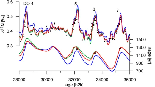
mate the shape of the modelledδ15N, (ii) refinement of the adjustment by varying the accumulation rate and a temperature shift for best fitting the∆_{age and (iii) final manual}

tuning where needed. The eﬀ_{ect of each step on the modelled}_δ15_{N and}∆_{age can be}

seen for the time period DO 4 to 7 in Fig. 1.

In the first step, 19 diﬀ_erent_α_{-scenarios have been calculated by varying the}_α_-value

25

in 0.02 steps from 0.24 to 0.60 %◦_C−1_{. As in Huber et al. (2006b) the initial}

(10)

CPD

9, 4099–4143, 2013

P. Kindler et al.

Title Page

Tables Figures

◭ ◮

Back Close

Full Screen / Esc

Discussion

P

a

per

|

D

iscussion

P

a

per

|

Discussion

P

a

per

|

Discuss

ion

P

a

per

|

introduced to match approximately the measured∆_{age. Without these corrections the}

modelled∆_{age is significantly underestimated in some parts, especially in the time}

pe-riod from 60 to 10 kyr. In order to find the bestα in a 2 kyr time window, the sum of the squared diﬀ_{erences between the}_δ15_{N model-output of a scenario and the spline}

through the measured data was calculated and the scenario with the smallest sum

5

was determined. Thereafter the time window was shifted continuously by 250 yr and the same procedure was applied until all data points were covered. At the end of step one, we obtain a “best”α-value every 250 yr, these values are splined for further cal-culations with a COP of 2 kyr. With these values, which vary roughly between 0.28 and 0.42 %◦_C−1_{, the model is able to reproduce coarsely the measured}_δ15_{N data (Fig. 1,}

10

blue lines).

To further refine the adjustment in a second step, the accumulation rate is varied from 60 to 100 % in 5 % steps and the temperature oﬀ_set _β _from +_{0 to} +_{8 K in 1 K}

steps while retaining theα-values from step one. This yields 81 diﬀ_{erent combinations}

and we proceed in the same way as in step one to find the best accumulation rate

15

and temperature shift to match the measuredδ15N data. The adjusted accumulation rate varies roughly from 70 to 80 % for 12 to 64 kyr, from 90 to 100 % for 64 to 92 kyr and from 80 to 100 % for 92 to 123 kyr. The time dependent temperature shiftβvaries within 2 K around+_{4 K. With these three tuned parameters (}_α_,_β_{and accumulation) the}

model is able to reproduce the measuredδ15N data generally well, both the amplitudes

20

as well as the timing of the DO events. The∆_{age output of the model and the calculated} ∆_{depth are also in agreement with the measured data (Fig. 1, green lines).}

The parts of the reconstruction which do not yet match are now tuned manually (on parametersβ and accumulation) on short periods (centuries) in a third step so that the model is able to reproduce the measured data within their uncertainty (Fig. 1, red

25

(11)

CPD

9, 4099–4143, 2013

P. Kindler et al.

Title Page

Tables Figures

◭ ◮

Back Close

Full Screen / Esc

Discussion

P

a

per

|

D

iscussion

P

a

per

|

Discussion

P

a

per

|

Discuss

ion

P

a

per

|

increased or decreased between the onset and the end of the event. In addition, the accumulation rate was enhanced or lowered slightly in these parts where the timing was not yet satisfactory. After step three, modelledδ15N as well as ∆_{age and}∆_depth

are in agreement with the measured data.

3 Results and discussion

5

The discussion is divided into four Sections. First we will discuss the new temperature reconstruction in Sect. 3.1, followed by simple consideration of theδ15N damping in the firn in Sect. 3.2. The used accumulation rate is reconsidered in Sect. 3.3 and finally we discuss theδ18Oice-temperature-relationship in Sects. 3.3.1 and 3.3.2.

3.1 Temperature

10

The reconstructed NGRIP temperature evolution from 10 kyr to 120 kyr b2k, together with the used δ18Oice data and the measured and modelled δ

15

N data, is shown in Fig. 2. The 2 sigma uncertainty linked to a temperature increase at the onset of a DO event is±3◦C (Huber et al., 2006b). The temperature evolution for the transition

Younger Dryas-Holocene (DO 0) to DO 8 is presented here the first time whereas the

15

temperature evolution for DO 9 to DO 25 is a reanalysis of existing data. Caution should be taken in the interpretation in the two temperature bumps occurring at around 80 kyr and 100 kyr, where the shape of the temperature curve diﬀ_{ers noticeably from the one}

of theδ18Oice signal (see Sect. 3.3).

To define the temperature amplitude of a DO event we had to specify the onset and

20

end of the event. The criterion to define the onset of a DO event corresponds to the diﬀ_{erence quotient exceeding 0.25}◦_{C/50 yr (0.05}◦_{C decade}−1_{), which is equivalent to}

about one-tenth of the increase rates for DO 9 to 17 found by Huber et al. (2006b). The end of the event was determined likewise, i.e. when the temperature increase rate became smaller than 0.05◦C decade−1. The 50 yr time interval was chosen because it

(12)

CPD

9, 4099–4143, 2013

P. Kindler et al.

Title Page

Tables Figures

◭ ◮

Back Close

Full Screen / Esc

Discussion

P

a

per

|

D

iscussion

P

a

per

|

Discussion

P

a

per

|

Discuss

ion

P

a

per

|

is long enough to overcome small-scale temperature variations. When one would use a longer time interval of 100 yr or longer, the durations of the temperature increases tend to be prolonged in an unrealistic way and the corresponding temperature ampli-tudes are in general slightly reduced.

With this method, we could well identify the start and end point of a DO event in

5

general. For the determination of the temperature amplitude at DO events, which fea-ture a two-step temperafea-ture increase, we had to apply the above mentioned criterion slightly diﬀ_{erently. Examples for such DO events are DO 2, 7 (Fig. 2c), 11 and 18.}

The duration of the small drop in temperature generally lasts for less than 100 yr and the amplitudes of less than 1◦C are quite small. As both sections of such a split

tem-10

perature increase exhibit about the same temperature increase rate they were treated as one increase, which means that the criterion of the 0.05◦_{C per decade was not}

applied during these small temperature reversals in between. Also DO 9 features ba-sically a stop (Fig. 2d). As the temperature plateau in this reconstruction is of longer duration (about 300 yr) than the following temperature increase (140 yr), the

tempera-15

ture plateau was not taken into account in our evaluation which leads to a∆_t=_{140 yr}

and∆_T=_6.5◦_{C. This is lower in amplitude than the findings from Huber et al. (2006b)}

that would be better in line when one includes the plateau resulting in∆_t=_{564 yr and} ∆_T=₈◦_{C. DO 5 may (Fig. 2b) also be considered to have a small temperature reversal}

at the beginning when one includes the 2◦C temperature drop just before the onset

20

of the DO event, resulting in ∆_t=_{473 yr and} ∆_T =_14.5◦_{C for DO 5. But when one}

looks closer to the onset of the DO event, the temperature reversal appears more to be some sort of plateau with a length of nearly 200 yr and the following temperature increase starts more gradual which is not the case in the temperature reversals of DO events mentioned above. So we exclude the small temperature drop before DO 5 from

25

our temperature increase calculations.

(13)

CPD

9, 4099–4143, 2013

P. Kindler et al.

Title Page

Tables Figures

◭ ◮

Back Close

Full Screen / Esc

Discussion

P

a

per

|

D

iscussion

P

a

per

|

Discussion

P

a

per

|

Discuss

ion

P

a

per

|

3500 yr (DO 17) and 2◦_{C in 2800 yr (DO 22). The long term warming before DO 8}

is comparable to the findings of Huber et al. (2006b) whereas they find a more pro-nounced long term warming of about 3 to 4◦C for DO 17. It is interesting to note that before each of the DO events in marine isotope stage (MIS) 3 which exhibit first a long-term warming a Heinrich event took place (H4, H5 and H6). This feature is shown in

5

Fig. 2 by the stadials marked with an orange background. Note that the colouring does not indicate the H events itself but the stadial where the event took place. The yellow shaded stadials, situated around the last glacial maximum, experience H events but do not manifest a long term warming before a DO event. The long term warming during H stadial 4 (before DO event 8) could be related to the findings of Jonkers et al. (2010),

10

who investigated northern North Atlantic (near) sea surface temperatures based on marine sediment cores during MIS 3. They observe a slight sea surface temperature increase during peak-ice rafting at H event 4 and probably also H event 5 and suggest that warm water from a subsurface heat reservoir reached episodically the surface during the warmer period of the year. The feature of a Greenland long term warming

15

during H stadial 4 could be of larger spatial extent as also Guillevic et al. (2013) found a slight long term warming during H stadial 4 at the NEEM site. Despite the fact that H events feature climatic changes in Europe (Genty et al., 2010; Sánchez Goñi et al., 2000), no particularly cold temperatures can be observed in our NGRIP temperature reconstruction during these stadial periods.

20

A linear relationship is observed between the length of the Greenland stadial and the temperature increase amplitude of the following AIM in Antarctica (EPICA commu-nity members, 2006; Capron et al., 2010a; Vallelonga et al., 2012). However, we do not observe a correlation between NGRIP temperature amplitudes and the duration of the preceding Greenland stadial (as defined by Capron et al., 2010a), or with the Antarctic

25

(14)

CPD

9, 4099–4143, 2013

P. Kindler et al.

Title Page

Tables Figures

◭ ◮

Back Close

Full Screen / Esc

Discussion

P

a

per

|

D

iscussion

P

a

per

|

Discussion

P

a

per

|

Discuss

ion

P

a

per

|

seesaw mechanism (Stocker and Johnsen, 2003) but are (also) governed by local ef-fects. Sea ice cover in the Arctic retreating during the DO warming may be a good candidate, as suggested by Gildor and Tziperman (2003) and Li et al. (2010).

Generally, the DO events feature temperature amplitudes between 9 and 13◦C which are independent of the background of the climate state (diﬀ_{erent MIS). The smallest}

5

temperature amplitude of 5◦C is obtained for DO 25. This is 2 degrees more than the result from Capron et al. (2012) but within their uncertainty of±2.5◦C. On the other

hand the largest amplitude of our temperature reconstruction is DO 11 with 16.5◦C, where Huber et al. (2006b) found a slightly smaller rise of 15◦C but still within the given uncertainty. Capron et al. (2010a) mentioned abrupt cooling events within DO event

10

24, these variations, according to our finding, can exceed 10◦_{C in about 150 yr.}

Deviations of our temperature reconstruction compared to other studies using the δ15N method can be explained by the application of diﬀ_{erent models (e.g. Goujon}

model, Goujon et al., 2003) and their adjustment to the measured data or by using a diﬀ_{erent approach, e.g. the combined use of} _δ15_{N and} _δ40_{Ar (Severinghaus et al.,}

15

1998; Landais et al., 2004b; Kobashi et al., 2011).

3.2 Damping of theδ15_{N signal in the firn}

Thomas et al. (2009) and Steﬀ_{ensen et al. (2008) investigated some transitions from}

stadials to interstadials on NGRIP ice using high resolution data (0.2 to 5 cm, corre-sponing to 3 yr or less) and found that some of these shifts can occur within a very

20

short time period. The warming seen in the δ18O_ice signal at DO 1 occurred within 3 yr (Steﬀ_{ensen et al., 2008) and the transition into the interstadial at DO 8 within 21 yr}

(Thomas et al., 2009). However, such rapid temperature increases cannot be seen in our temperature reconstruction. This may have two reasons: (i) as it is explained above, theδ18Oice data, which is used in the model input for a first temperature

esti-25

(15)

CPD

9, 4099–4143, 2013

P. Kindler et al.

Title Page

Tables Figures

◭ ◮

Back Close

Full Screen / Esc

Discussion

P

a

per

|

D

iscussion

P

a

per

|

Discussion

P

a

per

|

Discuss

ion

P

a

per

|

(ii) during extremely rapid events, theδ15N (especially theδ15Ntherm) formed at the LID

is damped by gas diﬀ_{usion in the firn and especially during the bubble close-o}ﬀ_process

that occurs over a depth interval of more than 10 m (Spahni et al., 2003), resulting in a smootherδ15N signal in the ice. This later eﬀ_{ect is included neither in the Schwander}

nor in the Goujon model (Schwander et al., 1997; Goujon et al., 2003).

5

Studying the transition from the Younger Dryas to the Holocene based onδ15N data from the GISP2 ice core, Grachev and Severinghaus (2005) smoothed the model out-put of a step function with a 40 yr moving average filter in order to take the gradual bubble enclosure into account. Apart from this publication we are not aware of other work where the damping in the firn is considered in connection with a δ15N-based

10

temperature reconstruction.

To investigate a possible influence of gas diﬀ_{usion and the gradual gas enclosure on}

the measuredδ15N signal during a rapid temperature rise, we modelled a basic and highly simplified scenario where the temperature was increased by+₁₀◦_{C (from} ₋₄₆

to−36◦C) with a concomitant accumulation increase from 0.06 to 0.10 m ice

equiva-15

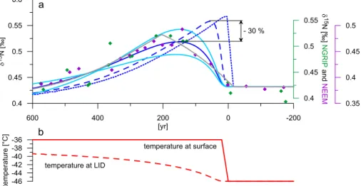
lent (m i.e.) within 20 yr according to our findings and those of Thomas et al. (2009) for DO 8. The result can be seen in Fig. 3a, where the dark blue dotted line represent the δ15N signal as calculated by the Schwander model which is then used as an input for the firn model from Spahni et al. (2003). With this model, which takes into account gas diﬀ_{usion and gradual bubble enclosure, one can assess the damping in the firn of an}

20

initial signal at the surface. The dark blue dashed line in Fig. 3a stands for the slightly smoothed signal after the gas diﬀ_{usion into the firn (as if the}_δ15_{N data were}

continu-ously measured at the LID) and the dark blue solid line for the final signal in the ice, after the gradual bubble enclosure. The dashed and the solid line scenarios were calcu-lated by folding the original signal (dotted line) with the characteristic age distribution of

25

(16)

CPD

9, 4099–4143, 2013

P. Kindler et al.

Title Page

Tables Figures

◭ ◮

Back Close

Full Screen / Esc

Discussion

P

a

per

|

D

iscussion

P

a

per

|

Discussion

P

a

per

|

Discuss

ion

P

a

per

|

to depths where the bubbles are enclosed altering the snow structure and therefore also the age distribution (Fig. 3b). Nevertheless, we accept this incompleteness in our simple calculation because at the time of the occurrence of the signal peak the temper-ature at the LID has only moderately changed. To allow for a small tempertemper-ature rise at the LID we use in our calculations an age distribution corresponding to−45◦C, slightly

5

higher than the original temperature of−46◦C. With these assumptions we find that for

the considered scenario (+₁₀◦_{C in 20 yr) the signal amplitude is damped by roughly}

30 % due to the gradual bubble enclosure process compared to the signal after the diﬀ_{usion into the firn.}

To compare the results of our simplified model calculations, we added measured

10

δ15N values of DO 8 both from NGRIP (green diamonds) and NEEM (violet diamonds), where a temperature increase of 8.8±1.2◦C has been found (Guillevic et al., 2013).

Note that the y-axes of the NGRIP and NEEMδ15N data have the same scale width compared to the y-axes of the modelled data but are shifted vertically in order to com-pare the shape of the signal evolution with the model simulations. The reason for the

15

vertical oﬀ_{set of the data can be found in the gravitational part of the} _δ15_{N, which is}

a characteristic of the individual firn depth of the site. To get an estimate of the sen-sitivity of the damping we added the light blue solid lines which represent the signal after the gradual bubble enclosure of a+_{7 and}+₁₃◦_{C temperature rise, respectively,}

according to our uncertainty of±3◦C of the temperature increase reconstruction.

20

As the measured data agree well with the shape of the solid lines, our simplified calculations indeed suggest a significant damping of the signal amplitude of roughly

−30 % due to the gradual bubble enclosure in the considered case. We refrain from

calculating the damping of longer temperature increases because of the added un-certainty due to the more increased temperature at the LID which complicates the

25

(17)

CPD

9, 4099–4143, 2013

P. Kindler et al.

Title Page

Tables Figures

◭ ◮

Back Close

Full Screen / Esc

Discussion

P

a

per

|

D

iscussion

P

a

per

|

Discussion

P

a

per

|

Discuss

ion

P

a

per

|

Also shown in Fig. 3a is the grey line which represents theδ15N signal as calculated by the Schwander model when the input data of the +₁₀◦_{C temperature increase is}

splined by 200 yr. One can see that the eﬀ_{ect of this initial smoothing of the input data}

(possibility (i) mentioned above), which was introduced to reduce the variability in the model output, is of similar magnitude as the eﬀ_{ect arising from the signal damping}

5

in the firn (possibility (ii)). Therefore we are confident that our reconstruction of the temperature amplitudes is still valid within the given uncertainty. This should also apply for other studies (Capron et al., 2010a; Guillevic et al., 2013; Huber et al., 2006b; Landais et al., 2005) whereδ18O_ice data smoothed up to 70 yr was used to estimate the corresponding site temperature.

10

For future work it is advisable to investigate the δ15N damping in the firn in more detail with transient models and a highly resolved measurement of an exemplary DO event (e.g. DO 1, 5, 8 or 19). Additionally, it would make sense to implement a grad-ual bubble enclosure process in firn densification and heat diﬀ_{usion models which are}

currently used to reconstruct the temperature evolution of a specific site. Also the

cal-15

culations forδ15Nthermshould be further refined in these models since the temperature

gradient, which is important for the determination of theδ15Ntherm, currently depends

only on two temperature points (top and bottom) and not on the actual temperature gradient itself. By this, the model may overestimate theδ15Ntherm at the beginning of

a temperature increase.

20

3.3 Accumulation rate

As mentioned in Sect. 2.2 and illustrated in Fig. 4, we had to significantly reduce the accumulation rate in some parts to adjust the modelledδ15N as well as∆_{depth and} ∆_{age to match the measured ones. From 12 to 64 kyr the accumulation was lowered}

by 20 to 30 % with a mean value of 24 %, from 64 to 92 kyr by 0 to 10 % with a mean

25

(18)

CPD

9, 4099–4143, 2013

P. Kindler et al.

Title Page

Tables Figures

◭ ◮

Back Close

Full Screen / Esc

Discussion

P

a

per

|

D

iscussion

P

a

per

|

Discussion

P

a

per

|

Discuss

ion

P

a

per

|

A comparison of our temperature reconstruction with reduced accumulation to a sce-nario with unchanged accumulation is shown in Fig. 4. The red lines show the used reduced accumulation rate and the corresponding modelled∆_{age and}∆_{depth values}

whereas the blue lines are obtained with an unchanged accumulation rate as described above in the Sect. 2.2 but without a final manual adjustment which would lead only to

5

minor changes regarding ∆_{age and} ∆_{depth values. One can clearly see that in the}

period from 10 to 60 kyr the 100 %-accumulation-scenario underestimates the ∆_age

by 50 to 500 yr and the ∆_{depth up to 8 m. Most significant deviations occur during}

the last glacial maximum. Not shown is the modelled δ15N data for the 100 % ac-cumulation rate-scenario, for which a substantial disagreement in the timing between

10

measured and modelled data occurs in this corresponding period (modelledδ15N val-ues are shifted to younger ages). According to our data adjustment, the accumulation reduction seems to be smaller in the older half of the record, nevertheless also here our model suggests in some periods (around 69, 83, 96 and 119 kyr, marked with grey bars in Fig. 4) a major reduction of 30 to 40 %.

15

A general test concerning accumulation rates and corresponding LID (which influ-ence the ∆_{age and}∆_{depth) can be performed with the Schwander model}

(Schwan-der et al., 1997). With the present-day NGRIP accumulation rate of 0.19 m i.e. yr−1 and a mean temperature of−31.5◦C (NGRIP members, 2004), the Schwander model

(Schwander et al., 1997) calculates a LID of 66.8 m, which is in excellent agreement

20

to measurements of 66 to 68 m (Huber et al., 2006a). Consequently, in absence of any warming event, the model is also able to calculate theδ15Ngrav. According to Figs. 2

and 4, the coldest temperatures of the reconstruction are around−55◦C and the lowest

accumulation rates are in the order of 4 cm i.e. yr−1. These are about the same values for Dome C present-day conditions: accumulation 2.7 cm i.e. yr−1and a temperature of

25

−54.5◦C (Landais et al., 2006). So we can consider the Dome C characteristics as

(19)

CPD

9, 4099–4143, 2013

P. Kindler et al.

Title Page

Tables Figures

◭ ◮

Back Close

Full Screen / Esc

Discussion

P

a

per

|

D

iscussion

P

a

per

|

Discussion

P

a

per

|

Discuss

ion

P

a

per

|

LID=_{98 m and} _δ15_N_grav=_{0.52 %}_{(Landais et al., 2006). Therefore we are confident}

that the Schwander model is capable of modelling NGRIP glacial climatic conditions and we suggest that the Dansgaard–Johnsen ice flow model (Dansgaard and Johnsen, 1969; NGRIP members, 2004) which was used to establish the NGRIP accumulation rate probably provides generally too high glacial accumulation rates, especially during

5

the coldest periods.

The fact that one has to reduce the NGRIP accumulation rate in some parts is not new. To reconstruct the temperature evolution from DO 9 to 17 (38 kyr to 64 kyr) Hu-ber et al. (2006b) reduced the accumulation rate from the ss09sea06bm time scale constantly by 20 %. When one averages our time dependent reduced accumulation

10

rate over the same period we get a similar value of 21.5 %. To test the validity of their model, Huber et al. (2006b) also modelledδ15N values of DO 18 to 20 (64 kyr to 79 kyr) measured by Landais et al. (2004a) and found that in this period one can use mostly the unchanged accumulation rate, which is also in line with our findings. Also Guillevic et al. (2013) who reconstructed the NGRIP temperature on DO 8, 9 and 10 (36.5 to

15

43 kyr on the GICC05 time scale), using the sameδ15N data but the Goujon firnifica-tion model (Goujon et al., 2003), had to reduce the accumulafirnifica-tion rate by 26 % in this section. Again, when averaged we find for the same period a similar accumulation re-duction of 28 %. Interestingly, Landais et al. (2004a, 2005) and Capron et al. (2010a, 2012) worked with the original accumulation rate to reconstruct the temperature

evolu-20

tion over DO 18 to 25. These findings are mostly confirmed by our work where we use accumulation rates of approximately 100 % around the DO events mentioned above. An exception is DO 24 for which we had to lower the accumulation rate by around 20 %. Back to 64 kyr, the ss09sea06bm time scale has been validated by the GICC05 annual layer counting time scale (Svensson et al., 2008), so in that time period the

25

(20)

CPD

9, 4099–4143, 2013

P. Kindler et al.

Title Page

Tables Figures

◭ ◮

Back Close

Full Screen / Esc

Discussion

P

a

per

|

D

iscussion

P

a

per

|

Discussion

P

a

per

|

Discuss

ion

P

a

per

|

As mentioned above, we had to significantly reduce the accumulation rate in the older half of the record during some periods (grey bars in Fig. 4). The decreased ac-cumulation rate leads to an increase in the modelled∆_age,∆_{depth (and temperature)}

in the corresponding periods (Figs. 4 and 5). Unfortunately, commonδ15N andδ18O_ice signals are missing. Therefore we are not able to check our modelled ∆_age,∆_depth

5

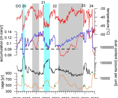
with measured data in these intervals. However, an indirect proxy for low accumulation rates is the dust content in the ice which shows in general elevated values during colder periods (Ruth et al., 2003) which are associated with low accumulation rates. Two of the four questionable low accumulation periods (83 and 96 kyr) mentioned above can be checked by dust data and are shown in Fig. 5 with grey bars on a depth scale.

10

As in Fig. 4 the blue line represents the unchanged accumulation and the red line the used reduced accumulation rate, respectively. The dust content is shown in black on a logarithmic scale and the modelled∆_{age in orange, green dots represent}∆_age

mea-surements. Highlighted with light blue one can see periods where low temperature and low accumulation rates are accompanied with clearly elevated dust contents. However,

15

this is not the case in the grey shaded periods although our modelled accumulation rates are as low as or lower than those of the stadial between DO 21 and 22 (shown by dashed line). A potential explanation for our accumulation reduction could be an overestimation of the time duration of these periods by the ss09sea06bm timescale. One can see in Veres et al. (2012) that the duration of the long DO 23, where we found

20

the most significant accumulation reduction, is about 1700 yr shorter on the new AICC 2012 time scale compared to the used ss09sea06bm time scale, probably because of a poorly determined thinning function near the bedrock (Veres et al., 2012). So, due to the fact that we were unable to confirm these four periods of low accumulation by the help of∆_{age and/or dust, caution should be taken by interpreting our accumulation}

25

(21)

CPD

9, 4099–4143, 2013

P. Kindler et al.

Title Page

Tables Figures

◭ ◮

Back Close

Full Screen / Esc

Discussion

P

a

per

|

D

iscussion

P

a

per

|

Discussion

P

a

per

|

Discuss

ion

P

a

per

|

3.3.1 δ18_O_ice_{-temperature relationship}

Before comparing the δ18O_ice data with our reconstructed temperature, the δ18O_ice data has been corrected for the influence of the increased isotopic composition of the ocean during the glacial after Jouzel et al. (2003):δ18Oicecorr=δ

18

Oice−∆δ 18

Osea·(1+

δ18O_ice)/(1+∆_δ18_O

sea). For this we used the∆δ 18

O_seafrom Bintanja et al. (2005) who

5

extracted from the benthic oxygen stack from Lisiecki and Raymo (2005) the isotopic signal in the ocean due to the increased ice masses at the poles.

The relationship betweenδ18O_icecorr and temperature can be seen in Fig. 6. In the top graph there is an overview over the glacial period (15 to 119 kyr) with anα-value (δ18Oicecorr to temperature-gradient) of 0.53 %◦C−

1

. As there are uncertainties in both

10

variables, the temperature and theδ18O_icecorr, we used the geometric mean regression to determine the gradients in this plot. In the four small graphs below, the relationship betweenδ18Oicecorr and temperature are shown for MIS 2 to 5 where it can be seen

that the dependency is varying through the glacial time. Huber et al. (2006b) found for the period 38 to 65 kyr a gradient ofα=_0.41_±_{0.05 %}◦_C−1_{, when we look at the same}

15

time interval we find 0.40±0.01 %◦C−1 which is in line with the results obtained from

Huber et al. (2006b). In the same paper, the smaller slope during MIS 3 compared to the modern times slope is explained by changes in annual distribution of precipitation (less winter precipitation in the stadial, more winter precipitation in a interstadial, re-spectively) and to a source temperature cooling (Fig. 4 in Huber et al., 2006b). The

20

fact that theδ18Oice is not only dependent on the mean annual temperature but also

amongst others on the seasonality of the precipitation has been previously discussed in Steig et al. (1994), Fawcett et al. (1997), Krinner et al. (1997), Masson-Delmotte et al. (2005) and Jouzel et al. (2007).

It has been proposed (Gildor and Tziperman, 2003; Kaspi et al., 2004) and shown

25

(22)

CPD

9, 4099–4143, 2013

P. Kindler et al.

Title Page

Tables Figures

◭ ◮

Back Close

Full Screen / Esc

Discussion

P

a

per

|

D

iscussion

P

a

per

|

Discussion

P

a

per

|

Discuss

ion

P

a

per

|

et al., 2005). This eﬀ_{ect is incorporated in the top graph of Fig. 6, where the}_δ18_O_icecorr

-temperature relationship data for the whole last glacial (15 to 119 kyr) is shown. The grey line indicates the modern Greenland spatial dependency of α=_{0.80 %}◦_C−1

between δ18Oice and temperature (Sjolte et al., 2011), the black line shows the

glacial δ18Oicecorr-temperature relationship calculated by the geometric mean

regres-5

sion method. The green and the red diamond represent glacial and modern mean values, respectively. As described in Huber et al. (2006b) and as we suggest it is the case in an interstadial, a precipitation source temperature cooling would shift the grey line to the left (dashed grey line), which means that less depleted precipitation is ex-pected. This can be understood by the help of a simple Rayleigh model: as the source

10

temperature gets colder when its location shifts towards north, the temperature gra-dient (and also the precipitation transportation distance) between source and site is smaller and therefore the isotopic composition is less depleted. The source tempera-ture cooling during interstadials is likely to be caused by the sea ice retreating around Greenland which allows high latitude water to evaporate and to serve as a

Green-15

land precipitation source (Masson-Delmotte et al., 2005). This shift to higher expected δ18Oice values during the interstadial is indicated in Fig. 6 by the blue line. Compared

to Huber et al. (2006b), we suggest a slightly diﬀ_{erent behaviour of the isotopic}

pre-cipitation during stadial conditions. As the sea ice extent is enlarged during stadial conditions (Broecker, 2000), the precipitation source location for Greenland

precip-20

itation is pushed southwards to warmer ocean conditions which can be traced in the d-excess (Masson-Delmotte et al., 2005). In addition to the lower stadialδ18Oicevalues

the expected isotopy should be further depleted because of the increased temperature gradient between precipitation source and the NGRIP site (Rayleigh), this suggested behaviour is shown in Fig. 6 by the red line. From that point of view, the discrepancy

25

between observed and expected δ18Oice values is even enlarged. We therefore

pro-pose that the seasonality eﬀ_{ect during stadials which is used to explain the mismatch}

(23)

CPD

9, 4099–4143, 2013

P. Kindler et al.

Title Page

Tables Figures

◭ ◮

Back Close

Full Screen / Esc

Discussion

P

a

per

|

D

iscussion

P

a

per

|

Discussion

P

a

per

|

Discuss

ion

P

a

per

|

3.3.2 Orbital control of theδ18_O_ice_{-temperature-sensitivity}

Here we investigate the δ18O_ice-temperature relationship at orbital time scales. For this, we calculated α (δ18Oicecorr-temperature-relationship) on a 10 kyr time window,

every 2 kyr (Fig. 7a), together with the corresponding correlation coeﬃ_{cient (}_R2_{). Blue}

dots correspond to time windows with a robust correlation (R2>0.70) and black dots

5

to time windows with a weaker correlation (0.47< R2<0.70), occurring generally in time periods with rare and small abrupt climatic changes. The calculatedα variations closely follow obliquity (Fig. 7a, green line, Berger and Loutre, 1991);αminima (around 0.3) correspond to obliquity maxima while alpha values reach up to 0.7 during obliquity minima. When looking at single DO events (1 kyr time window ending at the DO peak,

10

small grey diamonds in Fig. 7a), the variations are more scattered and theα-obliquity relationship is almost impossible to detect.

Vimeux et al. (1999) for Antarctica and Masson-Delmotte et al. (2005) for Greenland evidenced the imprint of obliquity in the source-site temperature gradient as visible in the d-excess records of polar ice cores. Indeed, a low obliquity implies an increase

15

of the source temperature and a cooling of the northern latitudes. The NGRIPδ18Oice

record and our reconstructed temperature profile (10 kyr spline, Fig. 7a, red line) clearly show minima in phase with obliquity minima. Cold Greenland temperature during obliq-uity minima is most probably further reduced by positive feedbacks such as extending sea ice and albedo eﬀ_{ects resulting in a further increase of the source-site temperature}

20

gradient.

The anticorrelation between α and obliquity that we observe cannot be explained by considering only the seasonality of the precipitation as in Masson-Delmotte et al. (2005) or Landais et al. (2004a). Indeed, in these studies, it is assumed that larger ice sheet (favoured by smaller obliquity) will strongly reduce the arrival of precipitation in

25

winter and hence increase the seasonality eﬀ_{ect, thus decreasing}_α_{. We observe the}

(24)

CPD

9, 4099–4143, 2013

P. Kindler et al.

Title Page

Tables Figures

◭ ◮

Back Close

Full Screen / Esc

Discussion

P

a

per

|

D

iscussion

P

a

per

|

Discussion

P

a

per

|

Discuss

ion

P

a

per

|

We suggest that the observed α-obliquity-relationship can be explained by a schematic Rayleigh distillation model (Fig. 7b), where the δ18O of precipitation is mainly explained by the source-site temperature gradient. In the case of an obliquity de-crease, we move on the Rayleigh precipitation curve from the right black dot to the left one, which exhibits a steeper gradient (Fig. 7b, blue line). This steeper gradient would

5

produce an enhanced isotopic eﬀ_{ect for the same temperature variation in Greenland,}

increasingα, which would be in agreement with our observations.

Interestingly, the amplitude ofα variations and the northern hemispheric ice sheets volume (Fig. 7a, black line, Bintanja et al., 2005) exhibit a concomitant increase from the Eemian to the Last Glacial Maximum. Note that the time uncertainty related to ice

10

sheet size data is 4 kyr (Lisiecki and Raymo, 2005). We therefore suggest that during obliquity minima,αmaxima are modulated by ice sheet size.

Moreover, while obliquity (and therefore also temperature) and α appear to be in phase at the beginning of the glacial period (110 kyr), one can observe an increasing lag of theα variations behind obliquity during the course of the glacial period ending

15

in a lag of roughly 10 kyr at 30 kyr. Note that calculatingα with diﬀ_{erent time windows}

(from 5 to 10 kyr) only slightly changes the position of theα peak at 20 kyr (±0.9 kyr).

Usingδ18O benthic data, Bintanja et al. (2005) and Waelbroeck et al. (2002) recon-structed the maximum ice sheet volume (or minimum sea-level) to be at around 20 kyr, where the dating uncertainty is±0.5 to 0.8 kyr (Waelbroeck et al., 2002). Taking into

ac-20

count the scatter in the diﬀ_erent_δ18_{O benthic records, a maximum uncertainty of}_±_{4 kyr}

seems reasonable. Theδ18O benthic lag compared to obliquity is still bigger than this uncertainty. Since the time lag ofα and ice sheet volume appear to be similar within dating uncertainty, this first continuous record ofα over a complete glacial-interglacial cycle confirms that Northern Hemisphere ice sheet volume influences the hydrological

25

(25)

CPD

9, 4099–4143, 2013

P. Kindler et al.

Title Page

Tables Figures

◭ ◮

Back Close

Full Screen / Esc

Discussion

P

a

per

|

D

iscussion

P

a

per

|

Discussion

P

a

per

|

Discuss

ion

P

a

per

|

δ18O level and (ii) be likely more sensitive to temperature fluctuations in Greenland. As a consequence,α would increase with the Laurentide ice sheet size volume, which is what we observe here.

4 Conclusions

In our NGRIP temperature reconstruction we presented for the first time a temperature

5

evolution from the Holocene to DO 8 based onδ15N measurements. In order to obtain a continuous temperature reconstruction for the whole glacial period (10 to 120 kyr b2k) we integrated all existingδ15N data in our reconstruction and found temperature rises during DO events ranging from +₅◦_{C (DO 25) to} ₊_16.5◦_{C (DO 11), which is in line}

with previous findings (Huber et al., 2006b; Landais et al., 2005; Capron et al., 2010a,

10

2012). Most of the DO events show a one-step temperature increase. In contrast, DO 2, 7, 11 and 18 feature a two-step temperature rise with a small interruption of generally less than 100 yr between stadial and interstadial conditions. Stadials where a Heinrich event is recorded in marine cores do not show a particularly cold temperature, during MIS 3 we even observe a long term warming of roughly one to three degrees during

15

Heinrich-stadials (H4, H5 and H6).

With a highly simplified model calculation we tried to assess theδ15N smoothing in the firn due to the gradual bubble enclosure and found a damping of−30 % for a+10◦C

temperature increase within 20 yr. Our smoothing of the model input data has an eﬀ_ect

which is in the same range. To be able to better quantify the damping in the firn in the

20

future, it would be advantageous to implement this eﬀ_{ect in the used firn densification}

and heat diﬀ_{usion models.}

In order to match measured and modelled δ15N data as well as ∆_{depth we had to}

reduce the accumulation rate given by the ss09sea06bm age scale significantly, partic-ularly in the second half of the last glacial from 12 to 64 kyr where a mean reduction of

25

(26)

CPD

9, 4099–4143, 2013

P. Kindler et al.

Title Page

Tables Figures

◭ ◮

Back Close

Full Screen / Esc

Discussion

P

a

per

|

D

iscussion

P

a

per

|

Discussion

P

a

per

|

Discuss

ion

P

a

per

|

model partly overestimates the NGRIP accumulation rate (Dansgaard and Johnsen, 1969; NGRIP members, 2004).

When comparing theδ18Oicecorrdata with the corresponding temperatures during the

last glacial and taking into account a warmer source temperature for the precipitation during stadials we propose that the seasonality eﬀ_{ect of precipitation during stadials is}

5

even more pronounced than previously assumed. An anticorrelation between obliquity and a long term (10 kyr)α has been found. Qualitatively, this is supported by a simple Rayleigh distillation model. We suggest that the amplitudes of theαvariations and their lag compared to obliquity are influenced by the northern hemispheric ice sheet volume. It would be interesting to use an isotopic model constrained by NGRIP isotopes and

10

our reconstructed temperature to distinguish between the variations ofα that can be explained by obliquity influencing the source-site temperature gradient (and therebyα), the ice-sheet volume eﬀ_{ect and the variations that would remain unexplained (possibly}

influenced by seasonality of precipitations, storm trajectories and fluctuations of Arctic sea-ice extent).

15

Acknowledgements. We thank Peter Nyfeler and Hanspeter Moret for their helpful assistance during the measurements in the laboratory. This work is a contribution to the NGRIP ice core project, which is directed and organized by the Ice and Climate Research Group at the Niels Bohr Institute, University of Copenhagen. It is being supported by funding agencies in Denmark (SNF), Belgium (FNRS-CFB), France (IPEV, INSU/CNRS and ANR NEEM), Germany (AWI),

20