Spatial gradients of temperature, accumulation and δ<sup>18</sup>O-ice in Greenland over a series of Dansgaard-Oeschger events

(1)

CPD

8, 5209–5261, 2012

Past spatial gradients of temperature andδ18_O

in Greenland

M. Guillevic et al.

Title Page

Abstract Introduction

Conclusions References

Tables Figures

◭ ◮

Back Close

Full Screen / Esc

Printer-friendly Version

Interactive Discussion

Discussion

P

a

per

|

Dis

cussion

P

a

per

|

Discussion

P

a

per

|

Discussio

n

P

a

per

|

Clim. Past Discuss., 8, 5209–5261, 2012 www.clim-past-discuss.net/8/5209/2012/ doi:10.5194/cpd-8-5209-2012

Climate of the Past Discussions

This discussion paper is/has been under review for the journal Climate of the Past (CP). Please refer to the corresponding final paper in CP if available.

Spatial gradients of temperature,

accumulation and

δ

18

_{O-ice in Greenland}

over a series of Dansgaard-Oeschger

events

M. Guillevic1,2, L. Bazin1, A. Landais1, P. Kindler3, A. Orsi4, V. Masson-Delmotte1, T. Blunier2, S. L. Buchardt2, E. Capron5, M. Leuenberger3, P. Martinerie6, F. Pri ´e1, and B. M. Vinther2

1

Laboratoire des Sciences du Climat et de l’Environnement, UMR8212, CNRS – Gif sur Yvette, France

2

Centre for Ice and Climate, Niels Bohr Institute, University of Copenhagen, Copenhagen, Denmark

3

Climate and Environmental Physics, Physics Institute and Oeschger Centre for Climate Change Research, University of Bern, Bern, Switzerland

4

Scripps Institution of Oceanography, University of California, San Diego, La Jolla, CA, USA 5

British Antarctic Survey, Cambridge, UK 6

(2)

CPD

8, 5209–5261, 2012

in Greenland

M. Guillevic et al.

Title Page

Tables Figures

◭ ◮

Back Close

Full Screen / Esc

Discussion

P

a

per

|

Dis

cussion

P

a

per

|

Discussion

P

a

per

|

Discussio

n

P

a

per

|

Received: 25 September 2012 – Accepted: 17 October 2012 – Published: 24 October 2012

Correspondence to: M. Guillevic (mgllvc@nbi.ku.dk)

(3)

CPD

8, 5209–5261, 2012

in Greenland

M. Guillevic et al.

Title Page

Tables Figures

◭ ◮

Back Close

Full Screen / Esc

Discussion

P

a

per

|

Dis

cussion

P

a

per

|

Discussion

P

a

per

|

Discussio

n

P

a

per

|

Abstract

Air and water stable isotope measurements from three Greenland deep ice cores (GISP2, NGRIP and NEEM) are investigated over a series of Dansgaard-Oeschger events (DO 8-9-10) which are representative of glacial millennial scale variability. Com-bined with firn modeling, air isotope data allow to quantify abrupt temperature increases

5

for each drill site. Our data show that the magnitude of stadial-interstadial temperature increase is up to 3◦C larger in Central and North Greenland than in North West Green-land. The temporal water isotope (δ18O) – temperature relationship varies between 0.3 and 0.6±0.08 ‰◦C−1 and is systematically larger at NEEM, possibly due to limited

changes in precipitation seasonality compared to GISP2 or NGRIP. The gas age-ice

10

age difference of warming events represented in water and air isotopes can only be modeled when assuming a 26 % (NGRIP) to 34 % (NEEM) lower accumulation than derived from a Dansgaard-Johnsen ice flow model.

1 Introduction

The last glacial period is characterized by rapid climatic instabilities at the millennial

15

time scale occurring in the Northern Hemisphere and recorded both in marine and terrestrial archives (Voelker, 2002; Bond et al., 1993). The NGRIP ice core, Northern Greenland, offers a high resolution water isotopes record where 25 rapid events were identified and described with a precise timing (NGRIP members, 2004). These events consist of a cold phase or stadial, followed by a sharp temperature increase of 9 to

20

16◦C at the NGRIP site as constrained by gas isotopes measurements (Landais et al., 2004a, 2005; Huber et al., 2006). Temperature then gradually cools down, sometimes with a small but abrupt cooling in the end, to the next stadial state. These temperature variations are associated with significant changes in accumulation rate, with annual lay-ers thicknesses varying by a factor of two between stadials and intlay-erstadials at NGRIP

25

(4)

CPD

8, 5209–5261, 2012

in Greenland

M. Guillevic et al.

Title Page

Tables Figures

◭ ◮

Back Close

Full Screen / Esc

Discussion

P

a

per

|

Dis

cussion

P

a

per

|

Discussion

P

a

per

|

Discussio

n

P

a

per

|

The identification of ice rafted debris horizons during stadials in North Atlantic sedi-ments (Heinrich, 1988; Bond et al., 1993; Elliot et al., 2001), together with proxy records pointing to changes in salinity (Elliot et al., 2001, 2002) and a reduced Atlantic Merid-ional Overturning Circulation (AMOC) (McManus et al., 1994; Rasmussen and Thom-sen, 2004), had led to the theory that DO events are associated with large scale

reor-5

ganizations in AMOC and inter-hemispheric heat transport (Blunier and Brook, 2001). The identification of a systematic Antarctic counterpart to each Greenland DO event (EPICA community members, 2006; Capron et al., 2010) fully supports this theory. This observation can be reproduced with a conceptual see-saw model using the Antarctic ocean as a heat reservoir and the AMOC as the way to exchange heat between

Antarc-10

tica and Greenland (Stocker and Johnsen, 2003).

Coupled atmosphere-ocean climate models are now able to reproduce the temper-ature pattern of DO events in Greenland in response to AMOC changes induced by freshwater forcing in the high latitudes of the Atlantic Ocean (Kageyama et al., 2010). However, modeled amplitudes of temperature changes are typically between 5 and

15

7◦C (Ganopolski and Rahmstorf, 2001; Li et al., 2005; Otto-Bliesner and Brady, 2010), significantly smaller than the temperature increase of 8–16◦_{C reconstructed based on}

ice cores data (Landais et al., 2004a; Huber et al., 2006). The correct amplitude of temperature change over the Bølling-Allerød is only reproduced in a fully coupled and high resolution atmosphere-ocean global circulation model (Liu et al., 2009). However,

20

a large part of the simulated warming is due to the simultaneous changes in atmo-spheric CO2 concentration and insolation, which are not at play for most DO events

of the last glacial period. This model-data mismatch motivates us to strengthen the description of the magnitude and spatial patterns of DO temperature changes, using different ice core sites. An improved regional description of past changes in Greenland

25

(5)

CPD

8, 5209–5261, 2012

in Greenland

M. Guillevic et al.

Title Page

Tables Figures

◭ ◮

Back Close

Full Screen / Esc

Discussion

P

a

per

|

Dis

cussion

P

a

per

|

Discussion

P

a

per

|

Discussio

n

P

a

per

|

isotopes) has been conducted over an array of drilling sites. This is the main target of this study.

In 2010 bedrock was reached at the deep ice core drilling site NEEM, in North West (NW) Greenland. A new deep ice core, 2.5 km long, is now available (Dahl-Jensen and NEEM community members, 2012). In this paper, we present new data from the

5

NEEM ice core together with existing and new measurements conducted on the GISP2 and NGRIP ice cores on DO events 8 to 10. The location of these drilling sites is depicted on Fig. 1 and their present-day characteristics are summarized in Table 1 (see also Johnsen et al., 2001). At present, the main source of NEEM precipitation is located in the North-Atlantic between 30◦N and 50◦N (Steen-Larsen et al., 2011). The

10

recent inter-annual variability of water stable isotopes (δ18O, δD) shows similarities with the variability of the Baffin Bay sea-ice extent. Unlike Central Greenland where snow falls year round, NW Greenland precipitation is simulated to occur predominantly in summer (Steen-Larsen et al., 2011; Sjolte et al., 2011; Persson et al., 2011). This specificity of the precipitation seasonality explains the particularly weak fingerprint of

15

the North Atlantic Oscillation in NEEM shallow ice cores (Steen-Larsen et al., 2011) compared to GISP2 (Barlow et al., 1993). These regional peculiarities are of particular interest, because past changes in precipitation seasonality are likely to affect water stable isotopes values.

Water isotopes are to a first order markers of local condensation temperature

20

changes at the precipitation site (Dansgaard, 1964). However, they are also affected by evaporation conditions, atmospheric transport and distillation, condensation con-ditions as well as seasonality of precipitation (Johnsen et al., 1989; Werner et al., 2000, 2001; Masson-Delmotte et al., 2005). They are thus integrated tracers of the hydrological cycle and quantitative indicators of past site temperature change, albeit

25

(6)

CPD

8, 5209–5261, 2012

in Greenland

M. Guillevic et al.

Title Page

Tables Figures

◭ ◮

Back Close

Full Screen / Esc

Discussion

P

a

per

|

Dis

cussion

P

a

per

|

Discussion

P

a

per

|

Discussio

n

P

a

per

|

Dahl-Jensen et al., 1998; Severinghaus and Brook, 1999; Lang et al., 1999; Johnsen et al., 2001; Landais et al., 2004a; Huber et al., 2006; Vinther et al., 2009).

Using the isotopic composition of nitrogen (δ15N) trapped in the ice bubbles allows to quantify the amplitude of past rapid temperature changes (e.g., Severinghaus and Brook, 1999; Landais et al., 2004a; Huber et al., 2006; Grachev and Severinghaus,

5

2005; Kobashi et al., 2011). At the onset of a DO event, the firn surface warms rapidly but its base remains cold because of the slow diffusion of heat in snow and ice. The resulting temperature gradient in the firn leads to thermal fractionation of gases: the heavy nitrogen isotopes migrate towards the cold bottom of the firn, where air is pro-gressively trapped into air bubbles. As a result, a sharp peak in δ15N is seen in the

10

gas phase as a counterpart to the rapid increase in water stable isotopes in the ice phase. Usingδ15N data and firn modelling, past surface temperature variations can be reconstructed (Schwander et al., 1997; Goujon et al., 2003). This method has already been applied to specific DO events on the NGRIP, GRIP and GISP2 ice cores (Lang et al., 1999; Huber et al., 2006; Landais et al., 2004a, 2005; Goujon et al., 2003;

Sev-15

eringhaus and Brook, 1999; Capron et al., 2010) and will be applied here for the first time to the NEEM ice core.

For this first study of regional variability of temperature changes over DO events, we focus on the series of DO events 8, 9 and 10 during Marine Isotopic Stage 3 (MIS3, 28–60 ka b2k, thousand years before 2000 AD). This period is indeed the most

20

widely documented for the millennial scale variability in a variety of natural archives. It is characterized by a large terrestrial ice volume (Bintanja et al., 2005), low atmo-spheric greenhouse gas concentration (Schilt et al., 2010), decreasing obliquity, low eccentricity and therefore small fluctuations in Northern Hemisphere summer insola-tion (Laskar et al., 2004). During MIS3, iconic DO events are particularly frequent, with

25

short lived interstadials (Capron et al., 2010) and constitute a clear target for model-data comparisons.

(7)

CPD

8, 5209–5261, 2012

in Greenland

M. Guillevic et al.

Title Page

Tables Figures

◭ ◮

Back Close

Full Screen / Esc

Discussion

P

a

per

|

Dis

cussion

P

a

per

|

Discussion

P

a

per

|

Discussio

n

P

a

per

|

reconstructions for NEEM and compare them with scenarios obtained with the same method for NGRIP and GISP2, investigating the water isotope-temperature relation-ships for these three different locations. We finally discuss the implications of our re-sults in terms of regional climate variations.

2 Method

5

2.1 Data

2.1.1 Nitrogen isotope data

The isotopic composition of nitrogen (δ15N) was measured on the NEEM core from 1746.8 to 1807.2 m depth at Laboratoire des Sciences du Climat et de l’Environnement (LSCE), France. We have a total of 97 data points with an average depth resolution of

10

62 cm corresponding to an average temporal resolution of ∼58 a. For this data set,

we have used a melt-refreeze technique to extract the air from the ice (Sowers et al., 1989; Landais et al., 2004b). The collected air is then measured by dual inlet mass spectrometry (Delta V plus, Thermo Scientific). Data are corrected for mass interfer-ences occurring in the mass spectrometer (Sowers et al., 1989; Bender et al., 1994).

15

Dry atmospheric air is used as a standard to express the results. The final pooled standard deviation over all duplicate samples is 0.006 ‰.

For the NGRIP core,δ15N was measured at the University of Bern (73 data points from Huber et al. (2006) and 36 new data points on DO 8). A continuous flow method was used for air extraction and mass spectrometry measurement (Huber and

Leuen-20

berger, 2004). The associated uncertainty is 0.02 ‰.

(8)

CPD

8, 5209–5261, 2012

in Greenland

M. Guillevic et al.

Title Page

Tables Figures

◭ ◮

Back Close

Full Screen / Esc

Discussion

P

a

per

|

Dis

cussion

P

a

per

|

Discussion

P

a

per

|

Discussio

n

P

a

per

|

(Orsi et al., 2012). In addition to these data, argon isotopes were also measured using the method from Severinghaus et al. (2003) (46 samples, pooled standard deviation of 0.013 ‰).

2.1.2 δ18_{O water isotope data}

We use the δ18O bag data (one data point corresponds to an average over 55 cm)

5

from the NEEM ice core measured at the Centre for Ice and Climate (CIC), University of Copenhagen, with an analytical accuracy of 0.07 ‰. For the NGRIP core, we use the bag data previously measured at CIC, with the same precision (NGRIP members, 2004). The GISP2δ18O data (20 cm resolution) are from Grootes et al. (1993) and are associated with an accuracy of 0.05 to 0.1 ‰.

10

2.1.3 Time scale

NEEM, NGRIP and GISP2 ice cores are all dated according to the Greenland Ice Core Chronology 2005, GICC05 (Vinther et al., 2006; Rasmussen et al., 2006; Andersen et al., 2006; Svensson et al., 2008). This time scale has been produced based on annual layer counting of several parameters measured continuously on the NGRIP,

15

GRIP and Dye3 ice cores and featuring a clear annual cycle, back to 60 ka b2k. The uncertainty at 38 ka b2k is 1439 a (MCE, Maximum Counting Error, Rasmussen et al., 2006). To transfer this time scale to the NEEM ice core, match points between peaks of electrical conductivity measurements (ECM) and di-electrical properties, measured continuously on the ice cores, have been used. The obtained time scale for NEEM

20

is called GICC05-NEEM-1 (S. O. Rasmussen, personal communication, 2010). The GISP2 core is matched to NGRIP using the same principle with match points from I. Seierstad (personal communication, 2012). The GICC05 age scale gives the age of the ice at each depth, and thus the annual layer thickness at each depth, but not the accumulation rate. This age scale is independent from estimation of thinning and past

25

(9)

CPD

8, 5209–5261, 2012

in Greenland

M. Guillevic et al.

Title Page

Tables Figures

◭ ◮

Back Close

Full Screen / Esc

Discussion

P

a

per

|

Dis

cussion

P

a

per

|

Discussion

P

a

per

|

Discussio

n

P

a

per

|

2.1.4 Accumulation rate

The Dansgaard-Johnsen (DJ) ice flow model (Dansgaard and Johnsen, 1969) calcu-lates the age and thinning function at each depth step (55 cm) along the ice core. The model parameters are tuned in order for the output time scale to match absolute age markers. Annual layer thicknesses given by the time scale are then divided by the DJ

5

thinning function to infer the accumulation rate. The NEEM version of the DJ model (Buchardt, 2009) is tuned in order to match the GICC05 time scale. For NGRIP, the ac-cumulation rate was first calculated using the ss09sea06bm age scale (Johnsen et al., 2001; Grinsted and Dahl-Jensen, 2002; NGRIP members, 2004). We re-calculated that accumulation according to the more accurate GICC05 time scale. Note that the

10

ss09sea06bm and the GICC05 time scales agree within the GICC05 uncertainty be-tween 28 and 60 ka b2k. For GISP2, the accumulation rate was first estimated with a 1 m resolution based on the coupled heat and ice flow model from Cuffey and Clow (1997) with the layer counted timescale from Alley et al. (1993), Meese et al. (1994) and Bender et al. (1994). This timescale has known issues in the vicinity of DO8 (Orsi

15

et al., 2012; Svensson et al., 2006) which causes the accumulation history derived from it to be also wrong. Orsi et al. (2012) used the layer thickness from the GICC05 timescale to re-calculate the accumulation history. Cuffey and Clow (1997) suggested 3 accumulation scenarios and Orsi et al. (2012) use the “200 km margin retreat” scenario adapted to the GICC05 timescale, compatible with the firn thickness and∆age derived

20

fromδ15N data. This accumulation scenario has also been proved to best reproduce ice sheet thickness variations (Vinther et al., 2009).

2.1.5 Ice-gas∆depth data

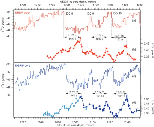
Figure 2 presents the NEEM δ15N profile over the sequence DO 8-10. The peaks of δ15N at 1769.4, 1787.5 and 1801.0 m are the result of the maximum

tempera-25

(10)

CPD

8, 5209–5261, 2012

in Greenland

M. Guillevic et al.

Title Page

Tables Figures

◭ ◮

Back Close

Full Screen / Esc

Discussion

P

a

per

|

Dis

cussion

P

a

per

|

Discussion

P

a

per

|

Discussio

n

P

a

per

|

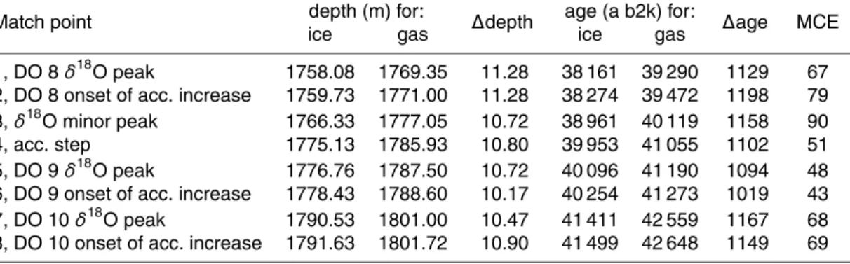
Sect. A2) and thus relate the maximum firn temperature gradient to the peaks inδ18 O-ice at 1758.1, 1776.8 and 1790.5 m. The depth differences between the temperature increases recorded in the gas and ice phases, named∆depth, can thus directly be in-ferred as 11.3, 10.7 and 10.5 m over DO 8, 9 and 10, respectively (Fig. 2, Table 2, points 1, 5 and 7, respectively). We propose another match point between weaker peaks of

5

δ15N andδ18O, see match point 3 in Table 2 and Fig. 6.

δ15N also increases with accumulation increase which deepens the firn (see Sect. 2.2) and we believe that this effect explains the beginning of δ15N increase at the onset of each DO event. Several abrupt transitions (Bølling-Allerød and DO 8) have been investigated at high resolution (Steffensen et al., 2008; Thomas et al., 2008), also

10

showing that the accumulation increases before theδ18O shifts with a time lead up to decades and ends after the completion of theδ18O increase. We observe the same feature for DO 8, 9 and 10 on the NEEM core. We thus match the onset of theδ15N increase at the beginning of DO events to the onset of accumulation increase, which occurs before the δ18O increase (Table 2 and Fig. 6, match points 2, 6, 8). Finally,

15

match point 4 is a step in accumulation that we relate to the same step seen inδ15N variations.

At NGRIP, DO 8, 9 and 10 are seen at 2086.6, 2116.2 and 2139.4 m in the gas phase and at 2068.0, 2099.1 and 2123.3 m in theδ18O from the ice phase (Fig. 2, Table 3 and Fig. 7, match points 2, 3, 4 respectively). For DO 8,δ18O shows a double peak and we

20

use the middle depth for this match point. We propose another match point at the end of DO 8 between wearker peaks ofδ15N andδ18O (match point 1). All these∆depth match points will be used in Sect. 3.1, combined with firn modeling, to reconstruct past surface temperature and accumulation.

2.2 Model description

25

(11)

CPD

8, 5209–5261, 2012

in Greenland

M. Guillevic et al.

Title Page

Tables Figures

◭ ◮

Back Close

Full Screen / Esc

Discussion

P

a

per

|

Dis

cussion

P

a

per

|

Discussion

P

a

per

|

Discussio

n

P

a

per

|

with theδ15N records (Schwander et al., 1997; Lang et al., 1999; Huber et al., 2006; Goujon et al., 2003; Landais et al., 2004a; Kobashi et al., 2011; Orsi et al., 2012). We here use the semi-empirical firnification model with heat diffusion by Goujon et al. (2003). This model, adapted to each ice core (see method Appendix A), calculates for each ice age and hence for each corresponding depth level the initial firn depth

5

(defined here as the depth where diffusion of gases stops i.e. lock-in-depth, LID), the age difference between ice and gas at the LID (∆age) and the temperature gradient between the bottom and the top of the firn. It is then possible to calculate theδ15N as the sum of two effects:

– gravitational effect: the heavy isotopes preferentially migrate towards the bottom

10

of the firn according to the barometric equation:

δ15_N

grav=exp

∆mgz RTmean

−1 (1)

with∆mthe mass difference between the light and heavy isotope,gthe acceler-ation constant,z the firn depth,R the ideal gas constant andT_meanthe mean firn temperature. An increase in accumulation rate increases the firn column depth

15

and therefore increasesδ15Ngrav; on the other hand, a high temperature

acceler-ates the densification processes and shallows the LID.

– thermal effect: the cold part of the firn is enriched in heavy isotopes according to:

∆δ15N_therm=

_T

t

Tb

αT

−1∼= Ω·∆T (2)

with T_t and T_b the temperatures of the top and bottom parcel respectively, α_T 20

(12)

CPD

8, 5209–5261, 2012

in Greenland

M. Guillevic et al.

Title Page

Tables Figures

◭ ◮

Back Close

Full Screen / Esc

Discussion

P

a

per

|

Dis

cussion

P

a

per

|

Discussion

P

a

per

|

Discussio

n

P

a

per

|

The model needs input temperature, accumulation and dating scenarios with a depth-age correspondence. In the standard version of the Goujon model, the temper-ature scenario is based on a tuned variable relationship between water isotopes and surface firn temperature, with:

T=_α1(δ18O+β) (3)

5

The reconstructed temperature has thus the shape of the water isotope profile but the temperature change amplitudes are constrained by tuning α and β in order for the modeledδ15N to match the measuredδ15N. Many earlier studies have shown that the temporal values of α are lower than the present day spatial slope for Greenland of 0.80 ‰◦_C−1

(Sjolte et al., 2011; Masson-Delmotte et al., 2011), which can be used as

10

a maximum value.

3 Results and discussion

3.1 Temperature and accumulation reconstruction

To reconstruct a continuous temperature and accumulation scenarios for DO 8 to 10, we run the firnification model from 60 to 30 ka b2k with a time step of one year and try

15

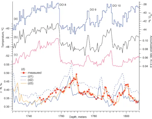
to reproduce theδ15N data as well as the ∆depth match points. Figure 3 shows the comparison between the measured and modeled (scenarios d1 to d3)δ15N over DO 8-10 at NEEM. First we try to reproduce theδ15N data by varying the temperature alone: the measuredδ15N amplitudes of DO 8, 9 and 10 can be reproduced with temperature increases at the GS-GIS (Greenland Stadial-Greenland Inter Stadial) transitions of 9.0,

20

6.0 and 7.7◦C respectively (Fig. 3, reconstruction d1). This scenario nicely reproduces both the meanδ15N level and the amplitude of theδ15N peaks. However, the modeled

(13)

CPD

8, 5209–5261, 2012

in Greenland

M. Guillevic et al.

Title Page

Tables Figures

◭ ◮

Back Close

Full Screen / Esc

Discussion

P

a

per

|

Dis

cussion

P

a

per

|

Discussion

P

a

per

|

Discussio

n

P

a

per

|

3.5◦C. This systematically deepens the LID, increasing both∆depth andδ15N (Fig. 3, reconstruction d2). The modeled∆depth is therefore closer to the measured one and the amplitude of theδ15N peaks is still correct but the meanδ15N level is systematically too high. From this experiment, we conclude that it is not possible to match bothδ15N data and∆depth by tuning only the temperature scenario.

5

Several explanations can be proposed to explain the underestimation of the∆depth by the model:

– the tuning of the Goujon model (LID density, vertical velocity field) is not appro-priate for the NEEM site and predicts a too shallow LID. However, we show in Appendix A3 that different tuning strategies have no impact on the modeled LID;

10

– the Goujon model is not appropriate for the NEEM site. However, this model is valid for present day at NEEM (see Appendix A1) and has also been validated for a large range of temperature and accumulation rates covering the expected glacial climatic conditions at NEEM (Arnaud et al., 2000; Goujon et al., 2003; Landais et al., 2006). Moreover, using other firnification models (the Schwander

15

model on NGRIP, Huber et al. (2006) and a Herron Langway model on NEEM, see Appendix C) with similar forcing in temperature and accumulation rate does not reproduce the measured∆depth either;

– fundamental parameters are missing in the description of current firnification mod-els. A recent study has shown that the firn density profile could be strongly

influ-20

enced by dust (calcium) concentration, the density increasing with the calcium concentration in the ice (H ¨orhold et al., 2012). During cold periods (glacials, sta-dials), the calcium concentration in Greenland ice cores is strongly enhanced compared to warm periods (interglacials, interstadials) (Mayewski et al., 1997; Ruth et al., 2007; Wolffet al., 2009). Taking this effect into account, the modeled

25

(14)

CPD

8, 5209–5261, 2012

in Greenland

M. Guillevic et al.

Title Page

Tables Figures

◭ ◮

Back Close

Full Screen / Esc

Discussion

P

a

per

|

Dis

cussion

P

a

per

|

Discussion

P

a

per

|

Discussio

n

P

a

per

|

This would further enhance the disagreement between modeled and observed

∆depth;

– the forcing in accumulation of the firnification model is not correct. To match the observed ∆depth with a correctly modeled δ15N, we need to significantly de-crease the accumulation rate compared to the original DJ estimation.

5

By adjusting changes in accumulation rate and the δ18O-temperature relationship (Fig. 3c and b), we manage to reproduce theδ15N profile as presented in Fig. 3, sce-nario d3. This best δ15N fit corresponds to a mean accumulation reduction of 34 % (30 to 40 %, depending on the DO event). Because the depth-age correspondence is imposed by the layer counting, this accumulation rate reduction by 34 % directly

im-10

plies the same 34 % decrease in the ice thinning. If we use this accumulation scenario as input for the DJ model, with keeping the original DJ accumulation scenario in the remaining ice core sections, the output time scale is just at the limit of the age uncer-tainty estimated by annual layer counting. For NGRIP, the Goujon model can reproduce the measuredδ15N profile with the correct ∆depth when using an accumulation rate

15

reduced by 26 % over the all section (Fig. 7). We further discuss past changes in accu-mulation rate in Sect. 3.4.

Based on these calculations, we conclude that reducing the accumulation scenario is necessary to match bothδ15N data and ∆depth with a firnification model over the sequence of DO 8-10; this reduction has no impact on the reconstructed rapid

temper-20

ature variations but requires to lower the mean temperature level by 3.5◦C for NEEM (2.5◦_{C for NGRIP). Our 26 % accumulation reduction for NGRIP supports the findings}

by Huber et al. (2006) where the original accumulation scenario was reduced by 20 %.

3.2 Uncertainties quantification

Following the same method for the 3 cores, we estimate the uncertainty (1σ)

associ-25

ated with the temperature increases∆T at the onset of the DO events to be ∼0.6◦C

(15)

CPD

8, 5209–5261, 2012

in Greenland

M. Guillevic et al.

Title Page

Tables Figures

◭ ◮

Back Close

Full Screen / Esc

Discussion

P

a

per

|

Dis

cussion

P

a

per

|

Discussion

P

a

per

|

Discussio

n

P

a

per

|

uncertainty is estimated to be∼0.05 ‰ for NEEM, 0.04 ‰ for NGRIP and 0.02 ‰ for

GISP2. The thermal sensitivity ofδ18O, defined asα= ∆δ18O/∆T, is associated with an uncertainty of 0.05, 0.08 and 0.02 ‰◦C−1 for NEEM, NGRIP and GISP2 respec-tively. The detailed calculations are given in Appendix B.

3.3 Regionalδ18_{O and temperature patterns}

5

Our best guess temperature and accumulation reconstructions for NEEM and NGRIP are displayed in Fig. 4 as a function of the GICC05 timescale. Our temperature re-construction for NGRIP is in excellent agreement with the one from Huber et al. (2006) where a different firnification model was used (see Fig. 7 in Appendix D). For the GISP2 core, we use the results from Orsi et al. (2012), where the temperature reconstruction

10

for DO 8 follows the same approach: temperature and accumulation scenarios are used as inputs to the Goujon firnification model and constrained usingδ15N andδ40Ar mea-surements (Orsi et al., 2012). Four different accumulation scenarios were used, with a stadial to interstadial increase of 2, 2.5, 3 and 3.5 times. The difference in tempera-ture increase between these four scenarios is very small (1σ=0.07◦C). We report in

15

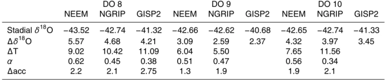
Table 4 the mean temperature increase for these four scenarios.

For a systematic comparison between the different ice core records, we have used a ramp-fitting approach (Mudelsee, 2000) to quantify the start, end and amplitude of DO increases inδ18O, temperature and accumulation: each parameter is assumed to change linearly between stadial and interstadial states. The magnitude of DO increases

20

are then estimated as the difference between the mean stadial and interstadial values (Table 4). The time periods used on each DO event for this statistical analysis are shown in Fig. 6.

3.3.1 Temperature sensitivity ofδ18_{O for present day and glacial climate}

For all three sites, the temporal sensitivity of water isotopes to temperature varies from

25

(16)

CPD

8, 5209–5261, 2012

in Greenland

M. Guillevic et al.

Title Page

Tables Figures

◭ ◮

Back Close

Full Screen / Esc

Discussion

P

a

per

|

Dis

cussion

P

a

per

|

Discussion

P

a

per

|

Discussio

n

P

a

per

|

gradient of 0.80 ‰◦C−1 (Table 4 and Sjolte et al., 2011). This can be explained by 2 main effects:

a. Source change effects: studies of the second order parameter deuterium excess suggest that the main source of water vapor is shifted southwards during the stadi-als (Johnsen et al., 1989; Masson-Delmotte et al., 2005; Jouzel et al., 2007; Ruth

5

et al., 2003). The enhancement of the source-site temperature gradient enhances isotopic distillation and produces precipitation with lowδ18O levels. Contradicting earlier assumptions (Boyle, 1997), conceptual distillation models constrained by GRIP deuterium excess data suggest that this effect is most probably secondary in explaining lower than present glacial slopes (Masson-Delmotte et al., 2005).

10

b. Precipitation intermittency/seasonality effects: at present, the NEEM area proba-bly receives 2 to 3.5 times more snow in summer than in winter (Steen-Larsen et al., 2011; Sjolte et al., 2011; Persson et al., 2011). This contrasts with the more year round distribution of snowfall at NGRIP and GISP2. Under glacial boundary conditions, atmospheric models depict a shift of Greenland precipitation towards

15

summer; this has been linked to a southward shift of the winter storm tracks due to the position of the Laurentide ice sheet (Werner et al., 2000, 2001; Krinner et al., 1997; Fawcett et al., 1997; Kageyama and Valdes, 2000). During cold pe-riods, summer snow may represent most of the annual accumulation, inducing a bias of the isotopic thermometer towards summer temperature and loweringα 20

compared to the spatial gradient (associated with a classical Rayleigh distillation). So far, seasonality changes have not been systematically investigated in climate model simulations aiming to represent DO events such as driven by freshwater hosing. In reduced sea-ice experiments by Li et al. (2005) using an atmosphere general circulation model, a 7◦_{C temperature increase and a doubling of the}

ac-25

(17)

CPD

8, 5209–5261, 2012

in Greenland

M. Guillevic et al.

Title Page

Tables Figures

◭ ◮

Back Close

Full Screen / Esc

Discussion

P

a

per

|

Dis

cussion

P

a

per

|

Discussion

P

a

per

|

Discussio

n

P

a

per

|

dust show synchronous annuals peaks during stadials for these species, whereas peaks occur at different periods of the year during interstadials, as for present-day (Andersen et al., 2006). This observation supports the hypothesis of a dramatic decrease of winter precipitations during stadials at NGRIP. No such high resolu-tion measurements are yet available for GISP2 and NEEM.

5

3.3.2 Regional differences between NEEM, NGRIP and GISP2

The magnitude of stadial-interstadial temperature rise is systematically increasing from NW Greenland to Summit (within uncertainties):+9.0◦C at NEEM,+10.4◦C at NGRIP and+11.1◦_{C at GISP2 for DO 8. For DO 10,} _∆_{T is largest at NGRIP and smallest at}

NEEM. For DO 9, temperature increases at NEEM and NGRIP are not significantly

10

different.

For each DO event, the amplitude of∆δ18O is decreasing from NW to Central Green-land: for DO 8,∆δ18O is 5.6 ‰ for NEEM, 4.7 ‰ for NGRIP and 4.2 ‰ for GISP2; the same pattern is seen for DO 9 and 10. As a result, the α coefficient decreases from NEEM to GISP2. The larger temporal values ofα encountered at NEEM are probably

15

explained by smaller precipitation seasonality effects for this site, which is already bi-ased towards summer at present day. In other words, because warm periods already undersample the winter snow at NEEM, a winter snow reduction during cold periods at NEEM cannot have an effect as strong as for the NGRIP and the GISP2 sites, where precipitation are distributed year-round for present-day. We note thatαdecreases with

20

site elevation (Table 1 and Table 4). Interestingly, the spatial pattern of DOα distribu-tion appears consistent with the spatial patterns of present-day inter-annual slopes (for summer or winter months), which are also higher in the NW sector (Sjolte et al., 2011). In addition to differences in seasonality/precipitation intermittency, differences in moisture transportation paths may also modulate the spatial gradients ofα over DO

25

(18)

CPD

8, 5209–5261, 2012

in Greenland

M. Guillevic et al.

Title Page

Tables Figures

◭ ◮

Back Close

Full Screen / Esc

Discussion

P

a

per

|

Dis

cussion

P

a

per

|

Discussion

P

a

per

|

Discussio

n

P

a

per

|

atmospheric general circulation models equipped with water tagging have indeed re-vealed different isotopic depletions related to the fraction of moisture transported from nearby or more distant moisture sources under glacial conditions (Werner et al., 2001; Charles et al., 2001). In particular, changes in storm tracks were simulated in response to the topographic effect of the Laurentide ice sheet, resulting in the advection of

5

very depleted Pacific moisture towards North Greenland. Indeed, systematic offsets between water stable isotope records of GRIP and NGRIP have been documented during the last glacial period (NGRIP members, 2004). So far, we cannot rule out that changes in moisture origin may cause differences inδ18O variations between NEEM, NGRIP and GISP2. Assessing the importance of source effects will require the

combi-10

nation of deuterium excess and17O excess data with regional isotopic modeling and remains beyond the scope of this manuscript.

3.4 Past surface accumulation rate reconstruction and glaciological implications

For NEEM and NGRIP (reduced accumulation) as well as GISP2 (original

accumu-15

lation), accumulation variations follow annual layer thickness variations: for each ice core, the smallest accumulation increase is seen for DO 9 and the largest one where the temperature increase is largest (DO 8 for NEEM, DO 8 and 10 for NGRIP). Accumu-lation shifts therefore scale with temperature variations (Table 4). This is in agreement with the thermodynamic approximation considering the atmospheric vapor content, and

20

thus the amount of precipitation, as an exponential function of the atmospheric tem-perature. Comparing the 3 sites, NEEM and NGRIP show similar accumulation rates whereas the accumulation is clearly higher at GISP2 over the all time period.

One important finding of our study is the requirement for a lower accumulation rate both at NEEM and NGRIP over DO 8-10, compared to the initial accumulation rate

25

(19)

CPD

8, 5209–5261, 2012

in Greenland

M. Guillevic et al.

Title Page

Tables Figures

◭ ◮

Back Close

Full Screen / Esc

Discussion

P

a

per

|

Dis

cussion

P

a

per

|

Discussion

P

a

per

|

Discussio

n

P

a

per

|

et al. (1997), also had to decrease the accumulation rate calculated by the DJ model by 20 % everywhere to fit the observed∆depth. Applying the Goujon model to the NGRIP ice core over DO 8-10, we found similar results. For GISP2 on DO 8, Orsi et al. (2012) used the Goujon model and an accumulation rate of 0.059 m.i.e.a−1for the stadial pre-ceding DO 8, as calculated by the ice flow model from Cuffey and Clow (1997) adapted

5

to the GICC05 time scale. In comparison, for the neighbouring GRIP site (28 km west of GISP2), the DJ model calculates an accumulation rate of 0.093 m.i.e.a−1 (50 % larger than GISP2) for the same period, while the present-day accumulation at GRIP is 8 % lower than at GISP2 (Meese et al., 1994; Johnsen et al., 1992). Such large differences in past accumulation rates between GISP2 and GRIP are not climatically plausible.

10

During the glacial inception, Landais et al. (2004a, 2005) were able to reproduce the measuredδ15N at NGRIP with the original time scale (ss09sea06bm, NGRIP mem-bers, 2004) and accumulation values from the DJ model. In the climatic context of the glacial inception, marked by higher temperatures compared to DO 8-10, firnification model and DJ ice flow models seem to agree.

15

Altogether, these results suggest that the DJ model is consistent with firn constraints during interglacials and inceptions, but a mismatch is obvious during DO 8-10, likely representative of glacial conditions. We now summarize three potential causes that could produce an overestimation of glacial accumulation in the DJ model (for a detailed presentation of this model we refer to Dansgaard and Johnsen, 1969).

20

a. Wrong age scale produced by the DJ model: the DJ model could underestimate the duration between two given depths in the ice core and thus overestimate the accumulation rate. However, for the NEEM ice core from present until 60 ka b2k, the DJ model is tuned in order to produce an age scale in agreement with the GICC05 time scale (Buchardt, 2009). For the NGRIP core, the ss09sea06bm time

25

(20)

CPD

8, 5209–5261, 2012

in Greenland

M. Guillevic et al.

Title Page

Tables Figures

◭ ◮

Back Close

Full Screen / Esc

Discussion

P

a

per

|

Dis

cussion

P

a

per

|

Discussion

P

a

per

|

Discussio

n

P

a

per

|

of accumulation reduction, assuming a systematic undercounting of the annual layers. For the glacial inception at NGRIP, Svensson et al. (2011) have counted annual layers on particular sections during DO 25 and the glacial inception and confirm the durations proposed by the ss09sea06bm time scale. We therefore rule out a possible wrong time scale as the main cause for the disagreement on

5

these particular periods.

b. The DJ model assumes a constant ice sheet thickness over time for NGRIP (Grin-sted and Dahl-Jensen, 2002) and a variable one for NEEM (ice sheet thickness reconstruction from Vinther et al., 2009). Here we investigate the effect of a pos-sible wrong ice sheet thickness history. Indeed, not taking into account a growing

10

(decreasing) ice sheet thickness leads to an overestimation (underestimation) of the thinning and therefore of the accumulation rate at the same period (e.g. Par-renin et al. (2007) for the EPICA Dome C site, Antarctica; Cuffey and Clow (1997) for the GISP2 site, Greenland). For the NGRIP core between 64 and 38 ka b2k, the time averaged accumulation rate according to ss09sea06bm is 0.084 m.i.e.a−1

15

and the one proposed by Huber et al. (2006) is 0.066 m.i.e.a−1. To explain the sys-tematic 20 % accumulation reduction, we would have to assume an average ice sheet growth at NGRIP from 64 to 38 ka b2k of 0.018 m.i.e.a−1 which leads to a total thickness increase of 468 m in 26 ka. For NEEM, the same calculation pro-duces a 210 meters thickness increase within 5 ka, between 43 and 36 ka b2k.

20

These numbers are unrealistic, several different models estimating the maximum ice sheet thickness change between glacial and interglacial to be∼200 to 250 m

at Summit (Letr ´eguilly et al., 1991; Cuffey and Clow, 1997; Huybrechts, 2002; Tarasov and Peltier, 2003; Vinther et al., 2009). To use enhanced ice sheet growth and retreat thus could help to explain part of the disagreement but cannot be its

25

single cause.

c. The DJ model assumes that the vertical velocity field (vz) changes only with

(21)

CPD

8, 5209–5261, 2012

in Greenland

M. Guillevic et al.

Title Page

Tables Figures

◭ ◮

Back Close

Full Screen / Esc

Discussion

P

a

per

|

Dis

cussion

P

a

per

|

Discussion

P

a

per

|

Discussio

n

P

a

per

|

(basal sliding, basal melt rate, kink height). Our need to reduce the DJ accumu-lation rate suggests thatvz is overestimated. In particular, a too deep kink height

produces an overestimation of the thinning and thus of the accumulation rate. The shape ofvzis actually expected to vary with the ice sheet temperature profile

through changes in ice viscosity (for more details we refer to Cuffey and Paterson,

5

2010, chap. 9). Under glacial conditions, we thus expect a reduced v_z, meaning a shallower kink height. During the Glacial Period, the connection between the Greenland Ice Sheet and the Ellesmere Island ice could also modify the Green-land ice flow. This effect is expected to more affect the ice flow at NEEM which is the closest site to Ellesmere Island, than at NGRIP and GISP2. In 1969 when

10

creating the DJ model to date the Camp Century ice core, the authors assumed a constant kink height over time due to a lack of information (Dansgaard and Johnsen, 1969). We conclude that the constant kink height used in the DJ model could explain why this model would not be appropriate to estimate correct thin-ning and accumulation rate over cold periods, despite the fact that this model has

15

been proved to produce accurate time scales. Firnification modeling may bring new constraints supporting the need for a variable kink height with time in the DJ model.

4 Conclusions and perspectives

Air isotope and water stable isotope measurements from three Greenland deep ice

20

cores (GISP2, NGRIP and NEEM) have been investigated over a series of Dansgaard-Oeschger events (DO 8-9-10) which are representative of glacial millennial scale vari-ability. We have presented the first δ15N data from the NEEM core and combined them with new and previously publishedδ15N data from NGRIP and GISP2. Combined with firn modeling, air isotope data allow us to quantify abrupt temperature increases

25

for each ice core site. For DO 8, the reconstructed temperature increase is 9.0◦_{C for}

(22)

CPD

8, 5209–5261, 2012

in Greenland

M. Guillevic et al.

Title Page

Tables Figures

◭ ◮

Back Close

Full Screen / Esc

Discussion

P

a

per

|

Dis

cussion

P

a

per

|

Discussion

P

a

per

|

Discussio

n

P

a

per

|

stadial-interstadial increase is up to 3◦_{C larger in central (GISP2) and North Greenland}

(NGRIP) than in NW Greenland (NEEM). The temporalδ18O temperature relationship varies between 0.3 and 0.6 ‰◦C−1and is systematically larger at NEEM, possibly due to limited changes in precipitation seasonality compared to GISP2 or NGRIP. The rela-tively high isotope-temperature relationship for NEEM will have implications for climate

5

reconstructions based on NEEM water isotopes data. Further paleotemperature inves-tigations are needed to assess the stability of this relationship over glacial-interglacial variations. In particular, it would be interesting to compare the presented reconstruc-tion with the temperature-water isotopes relareconstruc-tionship over the different climatic context of MIS 5. A better understanding of the causes of the regional isotope and temperature

10

gradients in Greenland requires further investigations of possible source effects (using deuterium excess and17O excess), and an improved characterization of atmospheric circulation patterns. We hope that our results will motivate high resolution simulations of DO type changes with climate models equipped with water stable isotopes, in or-der to test how models capture regional gradients in temperature, accumulation and

15

isotopes, and to understand the causes of these gradients from sensitivity tests (e.g. associated with changes in ice sheet topography, SST patterns, sea ice extent).

The gas age-ice age difference between abrupt warming in water and air isotopes can only be matched with observations when assuming a 26 % (NGRIP) to 34 % (NEEM) lower accumulation rate than derived from the Dansgaard-Johnsen ice flow

20

model. We question the validity of the DJ model to reconstruct past glacial accumu-lation rate and recommend on the time interval 42 to 36 ka b2k to use our reduced accumulation scenarios. We also suggest that the DJ ice flow model is too simple to reconstruct a correct accumulation rate all along the ice cores and propose to test the incorporation of a variable kink height in this model. Our results call for a

system-25

(23)

CPD

8, 5209–5261, 2012

in Greenland

M. Guillevic et al.

Title Page

Tables Figures

◭ ◮

Back Close

Full Screen / Esc

Discussion

P

a

per

|

Dis

cussion

P

a

per

|

Discussion

P

a

per

|

Discussio

n

P

a

per

|

species in the ice. Moreover, a better estimation of past surface accumulation rate at precise locations in Greenland would help to constrain past changes in ice flow with implications for ice sheet mass balance and dynamics.

Appendix A

The Goujon firnification model: method

5

The firnification model has only one space dimension and calculates the vertical veloc-ity field along the vertical coordinate and the temperature profile across the entire ice sheet for each time step of one year. In the firn, it calculates the density profile from the surface to the close-offdepth. The density profile and the accumulation history permit to obtain the ice age at LID, and assuming gas age equal to zero at LID, the∆age. The

10

temperature field from surface to bedrock is then used to reconstruct the density profile in the firn, the firn temperature gradient and from there theδ15N at LID. We follow Gou-jon et al. (2003) where the LID is defined as the depth where the ratio closed to total porosity reaches 0.13. The model is adapted to each ice core site in terms of vertical velocity field, basal melt rate, ice sheet thickness and elevation, and of course surface

15

temperature and accumulation scenarios (Table 1). We assume a convective zone of 2 meters at the top of the firn.

A1 Validation of the Goujon firnification model for present day at NEEM

We use the present day characteristics of the firn at NEEM to validate the Goujon firnification model. During the 2008 summer field season, a shallow core was drilled

20

(24)

CPD

8, 5209–5261, 2012

in Greenland

M. Guillevic et al.

Title Page

Tables Figures

◭ ◮

Back Close

Full Screen / Esc

Discussion

P

a

per

|

Dis

cussion

P

a

per

|

Discussion

P

a

per

|

Discussio

n

P

a

per

|

a clear convective zone. Below 62 m depth, δ15N is constant: the non-diffusive zone is reached. We thus have a LID of 62 m at NEEM for present-day according to these

δ15N data only. In Buizert et al. (2012), using measurements of different gases in the firn and several diffusion models, the S2 borehole is described as follow: a convective zone of 3 m, a diffusive zone of 59 m down to 63 m depth (LID), and a non-diffusive

5

zone down to 78.8 m depth (total pore closure depth). Following this description and assuming no thermal effect, we calculated the corresponding gravitational fractionation affecting δ15N; the corresponding profile is shown on Fig. 5, blue line. Annual layer counting of the corresponding shallow core and matching with the GICC05 timescale gives an ice age at LID of 190.6 a b2k±1 a and 252.5 a at the total pore closure depth.

10

The age of CO2is calculated to be 9.6 a at LID and 69.6 at the total pore closure depth,

producing a∆age of 181 a and 183 a respectively The best estimate for the true∆age is estimated to be 182+3/−9 a (Buizert et al., 2012). We observe that from the LID,

the∆age becomes constant within uncertainties. Considering the diffusion coefficient to be 1 for CO₂and using 1.275 for N₂as in Buizert et al. (2012), the age of N₂is 7.5

15

a at the LID, giving a∆age of 183 a.

We run the Goujon model using the NEEM07S3 shallow core age scale and δ18O for the top 60 m (Steen-Larsen et al., 2011) and the NEEM main core below. Theδ18O record is used to reconstruct the past temperature variations usingα=0.8 (Sjolte et al., 2011); we useβ=9.8 in order to obtain the measured average present-day

temper-20

ature of−29◦C (Steen-Larsen et al., 2011). Using the density profile measured along

the NEEM07S3 core and the corresponding age scale, the past accumulation history was reconstructed (Steen-Larsen et al., 2011), used here as input for the firnification model. The firnification model estimates the LID at 61.4 m depth. Modeledδ15N values agree well with the measured ones in this region (Fig. 5). At 63 m depth, the estimated

25

ice age is 189 a (according to the NEEM07S3 core dating, which agrees very well with the S2 core dating). Ignoring the gas age at LID thus results in an overestimation of the

(25)

CPD

8, 5209–5261, 2012

in Greenland

M. Guillevic et al.

Title Page

Tables Figures

◭ ◮

Back Close

Full Screen / Esc

Discussion

P

a

per

|

Dis

cussion

P

a

per

|

Discussion

P

a

per

|

Discussio

n

P

a

per

|

A2 Reconstruction of the past gas age scale

Simulations with the Goujon model shows that at the onset of DO events 8, 9 and 10, the heat diffusion in the firn is slow enough so that the peaks of maximum tempera-ture gradient in the firn are synchronous with theδ18O peaks. We thus consider that the peaks ofδ15N occur at the same time as the δ18O peaks. However, the Goujon

5

model has not gas diffusion component and this has two consequences: (a) the gas age at LID, due to the time for air to diffuse in the firn, is assumed to be zero; (b) any broadening of the initialδ15N peak by gas diffusion in the firn is not taken into account. For present day, the gas age at LID is 9.6 yr for CO2 (Buizert et al., 2012) and we

cal-culate it to be 7.5 a for N₂. The Schwander model calculates a N₂ age up to 20 a at

10

the LID over DO 8 to 10 for NGRIP (Huber et al., 2006). The Goujon model thus sys-tematically overestimates the∆age by 10 to 20 yr in the glacial period, which is within the mean∆age uncertainty of 60 yr (Table 2). For the NGRIP core, our temperature reconstruction with the Goujon model (without gas diffusion) is in agreement with the temperature reconstruction from Huber et al. (2006) where the Schwander model (with

15

gas diffusion) is used (Fig. 7). We thus consider that the lack of gas diffusion in the Goujon model has an impact which stays within the error estimate (Sect. B).

For DO8 to 10 at NEEM, we present the measured and modeledδ15N data plotted on an age scale on Fig. 6. The ∆age calculated by the model (Fig. 6, subplot d) is used to synchronize the gas record to the ice record. We have also reported here the

20

∆age tie-points from Table 2 and we can see that the modeled∆age reproduces these points, within the error bar.

A3 Sensitivity tests

A3.1 Vertical velocity field

In the firnification model, we used two different parameterizations for the vertical

veloc-25

(26)

CPD

8, 5209–5261, 2012

in Greenland

M. Guillevic et al.

Title Page

Tables Figures

◭ ◮

Back Close

Full Screen / Esc

Discussion

P

a

per

|

Dis

cussion

P

a

per

|

Discussion

P

a

per

|

Discussio

n

P

a

per

|

Goujon et al. (2003) and (b) a Dansgaard-Johnsen type vertical velocity field (Dans-gaard and Johnsen, 1969). In case (b), we used the same parametrization as the DJ model used to calculate past accumulation rate (ice sheet thickness, kink height, frac-tion of basal sliding, basal melt rate) and then tried different kink height between 1000 m and 1500 m above bedrock. All these tests produce the same modeled LID and hence

5

the same modeledδ15N. The different parameterizations actually produce very similar vertical velocity fields in the firn. Becauseδ15N is only sensitive to processes occurring in the firn, huge modification of the vertical velocity field deep in the ice (for example by modifying the kink height) has no impact here.

A3.2 Basal temperature

10

We also varied the basal temperature between−2.99◦C as measured at present in the

borehole (Simon Sheldon, personal communication) and−1.68◦C which is the melting

temperature as calculated in Ritz (1992) and can be considered as a maximum basal temperature. There is no difference in the modeled LID. Indeed, the relatively high accumulation rate even in the glacial period makes the burial of the snow layers quite

15

fast. As a result, the firn temperature is mostly influenced by the surface temperature but not by the bedrock temperature.

Appendix B

Uncertainties quantification

B1 Temperature increase

20

(27)

CPD

8, 5209–5261, 2012

in Greenland

M. Guillevic et al.

Title Page Abstract Introduction Conclusions References Tables Figures ◭ ◮ ◭ ◮ Back Close

Full Screen / Esc

Printer-friendly Version Interactive Discussion Discussion P a per | Dis cussion P a per | Discussion P a per | Discussio n P a per |

firnification. In a simple way, based on Eq. (2), we can write the temperature increase

∆T as:

∆T =∆δ 15

N_therm

DΩ (B1)

where∆δ15Ntherm is the differences in δ 15

Ntherm between stadial and interstadial, D

is a coefficient for the heat diffusion in the ice, Ω is the thermal diffusion sensitivity

5

(Grachev and Severinghaus, 2003).

To sum the uncertainties we use the general formula (Press et al., 2007):

σ_x=

s

σ_a2

_∂x

∂a

2

+σ_b2

_∂x

∂b

2

+σ_c2

_∂x

∂c

2

(B2)

where x is a function of a, b and c associated with respectively σa, σb and σc as

standard errors. We can thus sum the uncertainties associated to the temperature

10

increase:

σ_∆_T =

v u t

σ2

∆δ15_N therm

1

DΩ

2

+σ_Ω2

−∆δ15Ntherm Ω2_D

2

+σ_D2

−∆δ15Ntherm ΩD2

2

(B3)

orσ_∆T =

r

σ2

∆T,∆δ15_N

therm+σ

2 ∆T,Ω+σ

2

∆T,D (B4)

σ_∆T,∆δ15_N

therm: this uncertainty results from the analytical uncertainty for δ

15

N

mea-15

(28)

CPD

8, 5209–5261, 2012

in Greenland

M. Guillevic et al.

Title Page

Tables Figures

◭ ◮

Back Close

Full Screen / Esc

Discussion

P

a

per

|

Dis

cussion

P

a

per

|

Discussion

P

a

per

|

Discussio

n

P

a

per

|

stadial value (respectively 4, 3 and 1 points). For a stadial to interstadial increase, the

∆δ15N uncertainty is thus:

σ_∆_δ15_N =

v u u tσ

2

δ15_N nGS +

σ_δ215_N nGI

(B5)

which gives respectively 0.007, 0.006 and 0.007 ‰ for DO 8, 9 and 10. We run the firnification model with a modified temperature scenario in order to exceed the δ15N

5

peak value by 0.007 ‰ maximum, for each DO event. The accumulation scenario is kept unchanged. The obtained temperature increase is 0.58◦C larger. If we calculate

σ_∆_T,∆δ15_N as given by Eq. (B3) we obtain 0.52◦C. We conclude that the maximum

as-sociated temperature uncertainty is 0.58◦C. Concerning the validity of the firnification modeling, we have already shown in Sect. 3.1 that numerous tuning tests performed

10

with the Goujon model do not modify the estimated temperature increase. When using different firnification models (Schwander or Goujon) with similar inputs scenarios, the modeledδ15N profiles are similar. Moreover, the duration of temperature increase is well constrained by the GICC05 chronology and the high resolution δ18O data. The GICC05 dating and the identification of numerous∆age tie points (Table 2) between

15

gas and ice phase gives strong constrains on the accumulation scenario. We are thus quite confident in the validity of our firnification model to reconstruct past surface tem-perature and accumulation variations.

σ_∆T,D: since the duration of the temperature increase is very well known, the

un-certainty on the heat diffusion effect is thus rather small. In our case, it decreases the

20

firn temperature gradient by 1.66◦C with respect to a surface temperature increase of 9.02◦_{C for DO 8 for NEEM. The major uncertainty in the heat di}_ff_{usion model is linked}

to snow/ice conductivity modelisation. For the snow conductivity, we use the formula-tion from Schwander et al. (1997) where it is a funcformula-tion of the ice conductivity. We have tried different formulations for the ice conductivity (Weller and Schwerdtfeger, 1971;

25